Báo cáo hóa học: "Research Article Decentralized Utility Maximization in Heterogeneous Multicell Scenarios with Interference Limited and Orthogonal Air Interfaces" pot

Hindawi Publishing Corporation
EURASIP Journal on Wireless Communications and Networking
Volume 2009, Article ID 104548, 12 pages
doi:10.1155/2009/104548
Research Article
Decentralized Utilit y Maximization in
Heterogeneous Multicell Scenarios with Interference
Limited and Orthogonal Air Interfaces
Ingmar Blau,
1
Gerhard Wunder,
1
Ingo Karla,
2
and Rolf Sigle
2
1
Fraunhofer German-Sino Lab for Mobile Communications (MCI), Fraunhofer-Institute for Telecommunications,
Heinrich-Hertz-Institut, Einsteinufer 37, 10587 Berlin, Germany
2
Bell Labs, Alcatel-Lucent Deutschland AG, 70435 Stuttgart, Germany
Correspondence should be addressed to Ingmar Blau,
Received 6 August 2008; Revised 18 November 2008; Accepted 6 January 2009
Recommended by Mohamed Hossam Ahmed
Overlapping coverage of multiple radio access technologies provides new multiple degrees of freedom for tuning the fairness-
throughput tradeoff in heterogeneous communication systems through proper resource allocation. This paper treats the problem
of resource allocation in terms of optimum air interface and cell selection in cellular multi-air interface scenarios. We find a
close to optimum allocation for a given set of voice users with minimum QoS requirements and a set of best-effort users which
guarantees service for the voice users and maximizes the sum utility of the best-effort users. Our model applies to arbitrary
heterogeneous scenarios where the air interfaces belong to the class of interference limited systems like UMTS or to a class with
orthogonal resource assignment such as TDMA-based GSM or WLAN. We present a convex formulation of the problem and by

using structural properties thereof deduce two algorithms for static and dynamic scenarios, respectively. Both procedures rely on
simple information exchange protocols and can be operated in a completely decentralized way. The performance of the dynamic
algorithm is then evaluated for a heterogeneous UMTS/GSM scenario showing high-performance gains in comparison to standard
load-balancing solutions.
Copyright © 2009 Ingmar Blau et al. This is an open access article distributed under the Creative Commons Attribution License,
which permits unrestricted use, distribution, and reproduction in any medium, provided the original work is properly cited.
1. Introduction
In today’s wireless scenarios, new radio access technologies
(RATs) are emerging at frequent intervals. Although oper-
ators quickly introduce new wireless systems to the market
they still have a strong interest in exploiting their legacy
systems. Consequently, scenarios where an operator is in
charge of multiple air interfaces with overlapping coverage
are a common business case. Dense urban environments in
Europe, where users are often in the coverage of a cellular
TDMA-based GSM and CDMA-based UMTS systems, serve
as a good example. In this case, if services are offered
independently of the radio access technology and terminals
support multiple wireless standards, the operator has the
freedom to assign users to a cell and air interface of its choice.
Over the last years there has been growing interest
in academics and industry in which way these degrees of
freedom should be used and how users should be assigned
in heterogeneous wireless scenarios to exploit resources
more efficiently, incorporate fairness, and increase reliability.
Established concepts include load-balancing, service-based,
and cost-based strategies. Load-balancing strategies assign
users such that overload situations are avoided in one RAT
as long as there are resources left in a collocated radio system
[1]. More advanced approaches are service-based strategies

which select an RAT also in dependence of the requested
servicetype[2]. These strategies exploit the fact that one
wireless technology might be better suited to support a
certain service-class than another one due to different
granularities of distributable resources, different coding, and
modulation schemes. However, both approaches neglect the
fact that also the position and corresponding channel gain
of a user influence the efficiency of an RAT supporting a
service request. Reasons include different carrier frequencies
and corresponding channel models of RATs, base station
positioning, different interference situations and sensitivity
2 EURASIP Journal on Wireless Communications and Networking
to it. A concept that considers all earlier mentioned factors,
like the system load, service class, interference situation,
characteristics of the RAT, and users’ positions, is the cost-
based approach, introduced and analyzed in [3, 4]. There, it
was observed that all characteristics can be bundled together
in one cost parameter per user and RAT which suffice to
calculate a close to optimum assignment that maximizes
the total number of supportable voice users under static
conditions. Alternative approaches can be found in [5]and
references therein.
In this paper, we analyze in which way users of dif-
ferent service classes should be assigned in a heteroge-
neous scenario, thereby extending ideas from [3, 4]. Users
request either a fixed minimum data rate, for example,
as needed for voice services, or unconstrained best-effort
(BE) data services. We formulate the user assignment
as a utility maximization problem which is constrained
by the resources (such as power or bandwidth) of the

individual base stations (BSs) as well as users’ minimum
data rate requirements. The utilities represent quality of
service (QoS) indicators of the BE users and, by choosing
appropriate utility functions, give operators the freedom to
tune the operation point of the heterogeneous system. It
is important to note that although our model holds for
general concave utility functions we will adopt the concept
of α-proportional fairness introduced in [6] which allows to
variably shift the operation point between maximum sum
throughput, proportional fairness up to max-min fairness
by a single, parameterizable utility function. Related work
on utility maximization in nonheterogeneous interference
limited systems was carried out in [7–9], where the generally
nonconvex utility maximization problem was turned into
a convex representation (or supermodular game) using
specific techniques. The major difference to the approach
taken in this paper is that we consider a heterogeneous
scenario where the user-wise utilities are a function of the
individual link rates; this practical assumption significantly
complicates the analysis and neither of the approaches in
[7–9] can be applied. Based on the convex formulation and
by using structural properties, we present a decentralized
algorithm that solves the optimization problem for static
scenarios and derive simple assignment rules using the dual
representation of the utility problem. The insights gained
from the static setup are then adapted to dynamic scenarios
and we design a distributed protocol which requires minimal
information exchange between users and BSs and still
achieves considerable performance gains. Most importantly,
both algorithms allow operators to arbitrarily tune the

fairness-throughput tradeoff online without any system
changes. Although we cannot guarantee the convergence of
the simplified algorithm in the dynamic scenario we observe
a close to the global optimum operation in case a sufficient
number of users requests service and the variation of the
channel gains due to mobility is low. This is verified by the
derivation of an upper bound and comparison to simulation
results. Still, also for low service request rates and stronger
channel variations due to mobility and fading considerable
gains in terms of throughput and sum utility are obtained in
comparison to a load-balancing strategy.
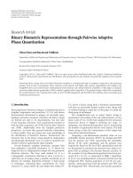
Investigation area
Movement area
Tr an sce iv er
Main transmission
direction
Figure 1: Playground with 40 GSM and 40 UMTS directional
transceivers (collocated).
The paper is organized as follows: after the introduction
of the system model and the utility concept in Section 2,
we will formulate the optimization problem in Section 3.
Algorithms that solve the problem in a decentralized way
for static and dynamic scenarios are presented in Section 4.
There, also the upper performance bound for the dynamic
scenario is derived. In Section 5,weeventuallyevaluatethe
performance of the dynamic algorithm by comparing it
to a load-balancing approach. We conclude the paper in
Section 6.
Notations. In this work bold symbols denote vectors or
matrices, calligraphic letters sets, and

|·|the cardinality of a
set. The transpose of a vector is (
·)
T
, x
m
is the mth element
of x,and
E(·) is the expectation. The summation over sets is
defined as X
=

n
X
n
={x : x =

n
x
n
, x
n
∈ X
n
}.
2. System Model
We consider a wireless scenario in the down-link direction
where multiple RATs with partly overlapping coverage are
arranged in an area called playground. The set of RATs A
=

A
orth
∪ A
inf
thereby consists of two subsets: in RATs with
orthogonal resources a
∈ A
orth
time or frequency slots or
subcarriers are assigned explicitly and users connected to one
BS do not interfere with each other. In interference limited
RATs a
∈ A
inf
all users share the same bandwidth and
the power constitutes the distributable resource. Each RAT
a
∈ A consists of a set of base stations m ∈ M
a
and one
operator is assumed to control the set of all base stations
M
=

a∈A
M
a
. An exemplary scenario with one cellular
UMTS system belonging to the interference limited class and
one cellular GSM/EDGE air interface of the orthogonal class

is depicted in Figure 1.
EURASIP Journal on Wireless Communications and Networking 3
Since commercial wireless systems usually operate on
individual frequency bands, we assume that signals of dif-
ferent RATs are orthogonal to each other and no intersystem
interference takes place. Users can be affected by intra- and
intercell interference within one radio technology, however.
The set of users I can be divided into two subsets
and users are equally distributed on the playground; users
i
∈ I
v
request a voice service with guaranteed data rate
and have priority to BE users i
∈ I
b
who do not have
any QoS guarantees. Furthermore, it is assumed that the
user equipment is able to cope with all RATs and the
service requests are independent of the technology giving the
operator the freedom to choose a cell and a RAT for each user
that is best suited from its perspective.
Next we will describe the two classes of RATs that are
covered in our scenario in more detail.
2.1. Orthogonal RATs. For the class of orthogonal systems
we assume a fixed transmission power per BS and that the
bandwidth, in terms of time or frequency slots, respectively,
is the resource continuously distributable between users.
Since commercial TDMA systems like GSM/EDGE usually
have low frequency reuse factors we will assume constant

intercell interference for this class of systems. The signal to
interference and noise ratio (SINR) of user i and a BS m of
this class
β
i,m
=
g
i,m
P
m
η
m
+ I
m
∀m ∈ M
a
, a ∈ A
orth,
(1)
thus depends on the channel gain g
i,m
, the BS power P
m
,
the constant intercell interference I
m
, the thermal noise η
m
,
and is independent of the assigned resource. The amount of

bandwidth assigned to user i by BS m is denoted by t
i,m
.Itis
limited by the total, distributable bandwidth per BS
T
m
and
the constraint

i∈I
t
i,m
= t
m
≤ T
m
∀m ∈ M
a
, a ∈ A
orth
. (2)
Due to the orthogonality of the users’ signals and since the
bandwidth is the distributable resource the relation between
auser’sdatarateR
i,m
and the assigned resource is linear for
this class of RATs:
R
i,m
= R

i,m
t
i,m.
(3)
Here,
R
i,m
:= f (β
i,m
) denotes the link rate per time or
frequency slot between user i and base station m where
f (β) is a positive, nondecreasing SINR-rate mapping curve
corresponding to the coding and transmission technology of
the RAT a
∈ A
orth
. By substituting (3) into (2) the achievable
rate region of each individual BS m
∈ M
a
results in an I-
dimensional simplex, limited by the positive orthant and a
hyperplane:
R
m
=

R
m
:


i∈I
R
i,m
R
i,m
≤ T
m
, R
i,m
≥ 0 ∀i ∈ I

,(4)
where R
m
is the i-dimensional vector with entries R
i,m
. Since
the rate assignment in one cell does not influence the feasible
rate region of neighboring cells the feasible rate region of the
whole RAT results in the convex polytope
R
a
=

m∈M
a
R
m
, a ∈ A

orth.
(5)
2.2. Interference Limited RATs. We assume that all users share
the same bandwidth and that resources are distributed in
terms of assigned power for BSs in interference limited air
interfaces like UMTS m
∈ M
b
, b ∈ A
inf
. The power of each
BS is limited by a sum constraint

i∈I
p
i,m
= P
m
≤ P
m
∀m ∈ M
b
, b ∈ A
inf,
(6)
where p
i,m
is the power that BS m assigns to user i ∈ I.
Users are sensitive to intracell and intercell interference in
interference limited systems and the SINR between BS m

∈
M
b
, b ∈ A
inf
and user i ∈ I is given by
β
i,m
=
g
i,m
p
i,m
ρg
i,m

j
/
=i
p
j,m
+

n
/
=m
g
i,n
P
n

+ η
inf
m, n ∈ M
b
, b ∈ A
inf
, i, j ∈ I,
(7)
with ρ the orthogonality factor which accounts for a reduced
intercell interference. In this class of systems all links of one
BS share a limited power budget and are impaired by the
power assigned to other users in the air interface. A well-
known model for the link rate of these systems is given in
[10]:
R
i,m
=C
b
log

1+D
b
β
i,m

=
C
b
log


1+D
b
g
i,m
p
i,m
ρg
i,m
(P
m
−p
i,m
)+

n
/
=m
g
i,n
P
n
+η
inf

.
(8)
There, the positive constants C
b
, D
b

parameterize the system
characteristics such as bandwidth, modulation, and bit-error
rates. In (8), a user’s data rate is in general neither convex
nor concave in p (index omitted). Therefore, also the feasible
rate region is not convex, which in turn will be a requirement
to obtain a convex representation of the utility maximization
problem in Section 3. However, assuming that all BS transmit
with fixed transmission power and that the SINR of all links
is not too high we can approximate the data rate by
R
i,m
= C
b
log

1+D
b
p
i,m
I
i,m
−ρp
i,m

≈
Δ
b
I
i,m
p

i,m
=: R
i,m
p
i,m
,
(9)
with
I
i,m
=
ρg
i,m
P
m
+

n
/
=m∈M
b
g
i,n
P
n
+ η
inf
g
i,m
. (10)

4 EURASIP Journal on Wireless Communications and Networking
0.10.080.060.040.020
p/I
R
= 1.14e9log
2
(1 + 8.7e −4 SINR)
Linear approximation: R
= 1.53e6 p/I
0
20
40
60
80
100
120
140
160
R (kbit/s)
Figure 2: UMTS resource-rate mapping: quality of linear approxi-
mation (9).
The approximation in (9) represents the first order Taylor
expansion for p
= 0 if one chooses Δ
b
= C
b
D
b
. Clearly,

this approximation holds only for low data rates and since
we are interested in a good approximation for typical rates of
the UMTS system, it turns out to be practical to use a higher
slope Δ
b
>C
b
D
b
. Indeed we plotted the rates in (9)overp/I
for UMTS in Figure 2 and chose Δ
b
so that it intersects the
real rate curve at the origin and 100 kbit/s which covers the
range of rates that are typically assigned to users in UMTS
in our scenario quite well. Obviously, this is only a model,
but works fine for the problem at hand. We refer also to the
discussion in Section 5.
By solving the approximation in (9)forp and substitu-
tion into (6) the achievable rate region of BS m
∈ M
b
can be
represented by
R
m
=

R
m

:

i∈I
R
i,m
R
i,m
≤ P
m
, R
i,m
≥ 0 ∀i ∈ I

. (11)
Since all BS are assumed to transmit with P
m
= P
m
,
the intercell interference is independent of the resource
assignment and the achievable rate region of the whole RAT
results in
R
b
=

m∈M
b
R
m

, b ∈ A
inf
, (12)
which is a convex polytope as for the orthogonal RAT.
Our approach stands in clear contrast to [8] where a
convex feasible rate region for interference limited RATs was
obtained with the posynomial transform and assuming R
≈
C log(Dβ). The posinomial approach has the advantage that
also the BS sum transmission power P
m
can be optimized.
However, the corresponding rate approximation is only valid
for high SINR and does not hold in our scenario. The linear
structure of our approximation will further lead to simple
assignment rules in Section 3.
2.3. Utility Concept and α-Proportional Fairness. Instead
of maximizing a fixed metric like the system throughput,
we will formulate the optimization problem in terms of
utility functions, which relate assigned resources, system
parameters as the SINR or the data rate to benefits such
as revenues, fairness or user satisfaction. More precisely,
we focus our investigations on utility functions which are
concave, strictly increasing and dependent on the user’s data
rate in the following form:
U
=

i∈I
b

ψ
i
⎛
⎝

m∈M
R
i,m
⎞
⎠
. (13)
Without loss of generality ψ
i
in (13)isgivenby
ψ
α
i

R
i

=
⎧
⎪
⎪
⎪
⎨
⎪
⎪
⎪

⎩
w
i
log

R
i

,ifα = 1,
w
i
1 −α
R
1−α
i
, otherwise.
(14)
Utilities defined by (13)and(14) correspond to the well-
established weighted α-proportional fairness [6], and are
from special interest for operators since they ensure flexible
tuning of the system fairness in a wide range. A rate
allocation R
∗
is said to be α-proportional fair, if for any
feasible allocation R

i∈I
b
R
i

−R
∗
i
R
∗
α
i
≤ 0 (15)
holds [6]. The parameter α in (14) hereby tunes the fairness-
throughput tradeoff;forα
= 0 the system throughput will
be maximized, which might result in assignments where
only very few users are served and which is quite unfair.
A selection α
= 1 leads to proportional fairness which is
equivalent to assigning equal shares of resources to all users
in our scenario. For α
→∞the assignment converges to the
max-min fairness, where all users will be assigned equal data
rates and the overall system throughput will be low [6].
Note that the definition of the utility in terms of the sum
ofauser’slinkratesin(13)ismorerelevantforpractical
application than, for example, the sum utilities of individual
links U
=

i

m
ψ(R

i,m
)usedin[7, 9]. It turns out that
it is exactly this so-called nonseparable utility formulation
that leads to the desired characteristic that most users will
establish only a single link, as will be shown in Section 3.By
contrast, the separable utility in [7, 9] will favor multilink
operation and therefore the results cannot be applied to our
model. This follows from the concavity of ψ and the Jensen’s
inequality; assume a user is assigned a certain sum rate R
i
that
can be split between two links R
i,m
and R
i,n
, R
i
= R
i,m
+ R
i,n
.
Then, it is beneficial in terms of the separable sum utility to
activate both links because ψ(R
i,m
)+ψ(R
i,n
) ≥ ψ(R
i
).

3. Problem Formulation
Having the system model and the utility concept introduced,
we now present the formal problem formulation. We want
to find the user assignment in a heterogeneous multicell
EURASIP Journal on Wireless Communications and Networking 5
scenario that maximizes the sum utility of all BE users under
the constraint that all voice users are assigned at least a
minimum data rate R
min,i
. Based on the earlier presented
assumptions, the problem can be formulated as
max
R

i∈I
b
ψ
i
⎛
⎝

m∈M
R
i,m
⎞
⎠
,
subject to

i∈I

R
i,m
R
i,m
≤ Γ
m
∀m ∈ M,

m∈M
R
i,m
≥ R
min,i
∀i ∈ I
v
,
R
i,m
≥ 0 ∀i, m ∈ I, M,
(P1)
with Γ
m
denoting available resources, Γ
m
= P
m
∀m ∈
M
b
, b ∈ A

inf
or Γ
m
= T
m
∀m ∈ M
a
, a ∈ A
orth
,
respectively. Problem (P1) consists of a concave objective
over linear constraints and is therefore convex. Consequently,
a variety of ready-to-use algorithms exists to solve it [11].
However, neither give these algorithms insights into the
problem structure nor do they give a hint to a decentralized
solution. We therefore develop a different approach based
on duality [11, 12]; instead of solving (P1) directly we
transform it into an alternative problem which is known
to have the same solution as (P1)butcanbesolvedin
a decentralized way. To obtain an expression for the dual
transform the Lagrangian function of (P1) is needed, which
has the following form:
L(R, λ,μ, σ)
=

i∈I
b
ψ
i
⎛

⎝

m∈M
R
i,m
⎞
⎠
−

m∈M
λ
m
⎛
⎝

i∈I
b
R
i,m
R
i,m
−Γ
m
⎞
⎠
+

i∈I
v
μ

i
⎛
⎝

m∈M
R
i,m
−R
min,i
⎞
⎠
+

i∈I

m∈M
σ
i,m
R
i,m
.
(16)
Here λ, μ, σ are nonnegative dual parameters. Next, we
introduce the dual function of (P1) which is defined as [11]
g(μ, λ, σ)
= max
R
L(R, μ,λ, σ). (17)
Due to nonnegativity of the dual parameters one observes
that (17) is always larger than or equal to the solution of (P1).

Therefore, minimizing the unconstrained dual function over
the dual parameters
min
μ,λ,σ≥0
g(μ, λ, σ) = min
μ,λ,σ≥0
max
R
L(R, μ,λ, σ)
  
inner problem
(18)
yields an upper bound on the original optimization problem
(P1) and is called the dual problem of (P1). Furthermore,
by convexity of (P1) and since Slater’s conditions [11]
hold, the bound is tight and (18)and(P1) have the same
solution. Our motivation to use the dual formulation is the
possibility to decouple the optimization problem into an
inner maximization problem over the primal variables R
and an outer minimization over the dual parameters which
will be called outer loop further on. Additionally, the dual
problem allows to exploit structural properties which will
greatly simplify the algorithm design. The inner problem
can be solved by each base station individually as we will
see shortly. In addition, there exists a very limited number
of degrees of freedom for the selection of meaningful dual
parameters in the outer loop. To be more precise, only λ
has to be optimized iteratively in the outer minimization. A
rate allocation R(λ) that maximizes the inner problem can
be calculated directly for a given λ independently of σ and μ.

Before we go into the details the KKT conditions are given,
which are necessary and sufficient for the optimum solution
of (P1) (or equivalently (18))[11] and will be exploited later:
∂L(R
∗
, μ
∗
, λ
∗
, σ
∗
)
∂R
i,m
= 0 ∀m, i ∈ M, I,
(19)
λ
∗
m
⎛
⎝

i∈I
R
∗
i,m
R
i,m
−Γ
m

⎞
⎠
=
0 ∀m ∈ M, (20)
μ
∗
i
⎛
⎝
R
min,i
−

m∈M
R
∗
i,m
⎞
⎠
=
0 ∀i ∈ I
v
, (21)
σ
∗
i,m
R
∗
i,m
= 0 ∀i, m ∈ I, M.

(22)
Here (
·)
∗
denotes the variables at the optimum.
3.1. Inner Problem. Rearranging terms in (16) results in the
following:
L(R, μ,λ, σ)
=

i∈I
b
ψ
i
⎛
⎝

m∈M
R
i,m
⎞
⎠
+

i∈I
v

m∈M
R
i,m


σ
i,m
−
λ
m
R
i,m
+ μ
i

+

i∈I
b

m∈M
R
i,m

σ
i,m
−
λ
m
R
i,m

+


m∈M
λ
m
Γ
m
−

i∈I
v
μ
i
R
min,i
.
(23)
From (23),oneobservesthat(17) is only finite if and only if
σ
i,m
−
λ
m
R
i,m
+ μ
i
= 0 ∀m, i ∈ M, I
v
,
(24)
λ

m
R
i,m
>σ
i,m
∀m, i ∈ M, I
b
,
(25)
and hence it follows that (24)and(25) are necessary condi-
tions to obtain a meaningful solution in (18). Furthermore,
the first KKT condition (19) has to hold for any rate
6 EURASIP Journal on Wireless Communications and Networking
assignment that solves (17) which after substituting (24) into
(23) simplifies to
∂L
∂R
i,m
= ψ

i


m∈M
R
i,m

+ σ
i,m
−

λ
m
R
i,m
= 0 ∀m, i ∈ M, I
b
.
(26)
Here, ψ

i
(x) = ∂ψ

i
(x)/∂x and (26) are necessary and
sufficient conditions for the maximum of the Lagrangian
function which is independent of the voice users. Although
the optimization of the dual parameters is formally per-
formed in the outer problem, one observes already here that
only certain σ can lead to the optimum solution of (P1).
More precisely, for a given λ only one element σ
i,m
can be
chosen freely for each user i so that (26) is not violated. All
other elements σ
i,n
, n
/
=m result directly from σ
i,m

by (26).
This is shown in the following example: assume one element
σ
i,m
and λ are given for user i from the outer loop. Then, for
the rate assignment that maximizes the inner problem u
i
:=
ψ

i
(

m∈M
R
i,m
) = (λ
m
/R
i
, m) −σ
i,m
has to hold (from (26)).
Since (26) is a necessary condition also for all n
/
=m it follows
that σ
i,n
= u
i

(σ
i,m
)+(λ
m
/R
i
, n), n
/
=m which is therefore
uniquely determined by σ
i,m
. This observation reduces the
degrees of freedom to select meaningful σ to one scalar
element per user in the outer loop. From (26), it further
follows that σ
i,m
= 0 can only hold for m ∈ M
opt,i
(λ), with
M
opt,i
(λ) =

m

i
∈ M : m

i
= arg min

m
λ
m
R
i,m

. (27)
This is a direct consequence of the nonnegativity of the dual
parameters and u
i
based on (26). Having σ
i,m
= 0, however,
is a necessary condition for R
∗
i,m
> 0 since for any optimum
rate assignment of (P1) the last KKT condition (22)hasto
be fulfilled. Therefore, regardless of the outer optimization
we can already state here that σ
i,n
> 0 ∀n
/
∈M
opt,i
, i ∈ I
b
and only rate assignments
R
i,m

⎧
⎪
⎨
⎪
⎩
≥
0 ∀m ∈ M
opt,i
(λ),
= 0 else
(28)
have to be considered as solution for (P1). Furthermore,
setting σ
i,m
= 0 m ∈ M
opt,i
if possible is required to allow
for assignments with R
i,m
> 0. Only if the maximum slope of
the utility function ψ

(0) is smaller than min
m
(λ
m
/R
i,m
) this
will result in σ

i,m
> 0 ∀m ∈ M
opt,i
then so that (26)isnot
violated. In this case user i will not be assigned any resources.
The KKT conditions lead to similar optimality conditions for
the voice users; from (24) as well as the argumentation above
it follows that
μ
i
= min
m
λ
m
R
i,m
∀i ∈ I
v
, (29)
and that (28) is also a necessary condition for the voice users.
It is noted here that for a given λ the solution of (17)is
uniquely determined (see proof of Theorem 1 in Section 4).
However, the corresponding rate assignment might not be
unique. Multiple optimum rate assignments can exist in the
rare case when
∃{m, n ∈ M, m
/
=n : λ
m
/R

i,m
= λ
n
/R
i,n
} and
therefore
|M
opt,i
(λ)| > 1. For all other users it follows by (26)
and the discussions on σ that the rate assignment
R
i,m
(λ) =
⎧
⎪
⎪
⎪
⎪
⎪
⎪
⎪
⎪
⎪
⎪
⎪
⎪
⎪
⎪
⎨

⎪
⎪
⎪
⎪
⎪
⎪
⎪
⎪
⎪
⎪
⎪
⎪
⎪
⎪
⎩
ψ
−1
i

λ
m
R
i,m
i

if ψ

i,m
(0) >
λ

m
R
i,m
,
m
∈ M
opt,i
(λ), ∀i ∈ I
b
,
R
min,i
if m ∈ M
opt,i
(λ), ∀i ∈ I
v
,
0 else
(30)
maximizes the inner problem and solves (17). In this case, the
rate assignment is unique and only depends on λ.In(30),
ψ

−
1
is the inverse of the derivative of the utility function
with ψ

(ψ


−
1
(x)) = x.
Equation (30) gives some valuable insights to the opti-
mum cell/RAT selection of users and the corresponding
resource assignment. First, it can be shown that almost all
users are assigned to exactly one BS since
|M
opt,i
|=1in
general. Second, this BS can be determined independently
by each user if λ is known and under the assumption that
each user i can measure
R
i.m
∀m ∈ M.Bothcharacteristics
rely on the linear connection between the data rate and the
assigned resources and on the user based utilities and greatly
simplify the distributed solution of (P1). In contrast, one
would obtain that R
∗
i,m
> 0 ∀i, m ∈ I, M
b
, b ∈ A
inf
under
the high SINR assumption in [7, 9], which implies that all
users have active connections to all BSs in the interference
limited air interface. Third, the maximum slope of the utility

function ψ
i
(0) defines a threshold which can be tuned to
switch off BE users with low
R
i,m
, as will be described in
Section 5.
3.2. Outer Problem. Since for μ (24) has to hold, λ and
formally σ are the only dual parameters that have to be
considered in the outer optimization. In order to minimize
the dual (17), clearly all entries of σ have to be as small
as possible and chosen in a way that (26) holds. Therefore,
σ
i,m

i
= 0 ∀{i, m

i
: i ∈ I
b
, m

i
∈ M
opt,i
(λ), λ
m


i
/R
i,m

i
≤ ψ(0)}.
A subgradient approach can be applied to minimize the dual
over λ [12]. Assume for a given

λ

R = arg max
R
L(R,

λ) (31)
is the solution of inner problem, obtained by (30). Then, the
following holds for the dual function [12]
g(λ)
≥L(

R, λ)=L(

R,

λ)+

m∈M

λ

m
−

λ
m

⎛
⎝
Γ
m
−

i∈I

R
i,m
R
i,m
⎞
⎠
,
(32)
where the last equation is obtained by adding and subtracting
the terms

m∈M

λ
m
(Γ

m
−

i∈I
(

R
i,m
/R
i,m
)) to L(

R,

λ)and
the assumption that σ
i,m
R
i,m
= 0 ∀i, m ∈ I, M. Further,
EURASIP Journal on Wireless Communications and Networking 7
it can be shown from (32) that the vector ν,withν
m
=
(Γ
m
−

i∈I
(


R
i,m
/R
i,m
)) is a subgradient.
A descriptive explanation of the subgradient approach
is as follows: for a given

λ
/
=λ
∗
the rate assignment

R
might either violate the feasible rate region constraint or
will not exploit all available resources. Both cannot be
optimal since the first case is not feasible and in the
latter case the assignment of more resources to any BE
user would increase the sum utility. Then, the subgradient
gives the direction how λ should be updated so that the
resource constraints are less violated or more resources are
assigned. At the global optimum of (P1), all entries of
the subgradient will be zero and all resource constraints
are met with equality. The subgradient will be used in
the decentralized algorithm, which will be presented in
Section 4.
4. Algorithm
We will now present two decentralized algorithms for

(P1)inastaticanddynamicscenario,respectively.In
the static setup, all user requests and channel gains are
assumed to be fixed, while in the dynamic one the requests
and user mobility are subject to stochastic processes.
The static algorithm hereby serves as motivation for the
dynamic one which is adapted for practical applications with
the advantage of requiring almost no signaling informa-
tion.
4.1. Static Scenario. Based on the optimality conditions of
the inner problem and the subgradient of the outer loop in
Section 3, we are able to formulate the static Algorithm 1,
where l denotes the index of the iteration, δ(l) is the step
size, and
 a constant for the stopping criteria. The algorithm
consists of an iterative procedure where in each cycle at first
all BSs broadcast the BS weights λ
m
to all users. Then, each
user i evaluates λ
m
/R
i,m
for all BSs and sends an assignment
request (and the corresponding
R
i,m
or R
min,i
)toaBSm


i
∈
M
opt,i
.Next,eachBSm individually calculates the rate
assignment for all users that sent an assignment request to
it. The rate assignment hereby depends on λ
m
and might lie
either inside, on, or outside the feasible rate region of BS
m and thereby either under exploit, meet with equality or
violate the resource constraint. Correspondingly, BS m will
update λ
m
using the subgradient and the cycle starts again by
broadcasting the updated BS weight. Although Algorithm 1
might not converge to the optimum rate assignment in case
∃{m, n ∈ M, m
/
=n : λ
∗
m
/R
i,m
= λ
∗
n
/R
i,n
} and therefore

results in
|M
opt,i
(λ
∗
)| > 1, we can formulate the following
theorem.
Theorem 1. Assume that for the series lim
l →∞
δ(l) =
0, lim sup
l →∞

l
δ(l) =∞holds and that a feasible allocation
for the voice users exists, then Algorithm 1 converges to the
optimum dual weights λ
∗
.Incase|M
opt,i
(λ
∗
)|=1 ∀i ∈ I the
corresponding rate assignment of Algorithm 1 is also optimal.
In case
∃i ∈ I : |M
opt,i
(λ
∗
)| > 1 an optimum rate assignment

that solves (P1) can be obtained by solving the set of linear
equations:

m∈M
opt,i
R
∗
i,m
= ψ

−
1

min

min
m
λ
∗
m
R
i,m
, ψ

i
(0)

, ∀i ∈ I
b
,


m∈M
opt,i
R
∗
i,m
= R
min,i
, ∀i ∈ I
v
,

i∈I
R
∗
i,m
= Γ
m
, ∀m ∈ M.
(33)
Proof. In Section 3.1, it was shown that steps (3) and (4)
of Algorithm 1 maximize the inner problem of (18)incase
|M
opt,i
(λ)|=1 ∀i ∈ I. Step (5) corresponds to an update of
λ in direction of the negative subgradient which was derived
in Section 3.2. Since (P1) is a convex optimization problem
and Slater’s condition holds, it is proven in [12] that the
dual problem (18) has the same solution as (P1). Further,
it is shown in [12] that dual subgradient algorithms like

Algorithm 1 converge to the global optimum for the given
step-width constraints. The proof can be extended to the case
where
∃i ∈ I : |M
opt,i
(λ)| > 1 by observing the fact that
the maximum of the inner problem is independent of the BS
m
i
∈ M
opt,i
which is selected by user i in step (3) (however,
it clearly matters for complying with the feasible rate region
constraints); from (26) it follows that
R
i
=

m
R
i,m
= ψ

−
1

λ
m
R
i,m

−σ
i,m


 
ζ
i
∀m, i ∈ M, I
b
(34)
is necessary and sufficient for the maximization of the inner
problem and that by (21)

m∈M
R
i,m
= R
min,i
∀i ∈ I
v
holds.
Substituting this into the Lagrangian (23) together with (24)
results in a dual function
g(λ)
=

i∈I
b
ψ


ψ

−
1

ζ
i

−

i∈I
b
ζ
i
ψ

−
1

ζ
i

+

m∈M
λ
m
Γ
m
−


i∈I
v
μ
i
R
min,i
,
(35)
which is independent of the actual BS selection of the users.
Therefore, Algorithm 1 will converge to the optimum λ
∗
and
to the maximum utility also if
∃i ∈ I : |M
opt,i
(λ)| > 1.
The optimum rate assignment of users that are in multilink
operation results then from λ
∗
by solving the set of KKT
conditions which reduce to (33) since λ
∗
m
> 0 ∀m ∈ M, μ
i
>
0
∀i ∈ I
v

for any nontrivial solution.
4.2. Dynamic Scenario. In a dynamic scenario where users
and service requests follow stochastic mobility and traffic
models, respectively, applying Algorithm 1 might be a good
choice from a theoretic perspective. Practically, however,
the procedure is too expensive, since, having the optimum
user assignment at any point in time, it would have to
be executed any time a user’s channel gain or interference
8 EURASIP Journal on Wireless Communications and Networking
(1) Each BS initializes λ
m
, ν
m
= 1 ∀m ∈ M, l = 0.
while !((ν(ν)
T
> )||(l<l
max
)) do
(2) Each BS broadcasts λ
m
to all users.
(3) Each user i
∈ I evaluates M
opt,i
(λ)with(27) and announces an assignment request to
m

i
(λ) ∈ M

opt,i
(λ). If |M
opt,i
(λ)| > 1 it picks one BS of the set randomly.
(4) Based on the assignment requests each BS calculates the rate assignment that maximizes its
sum utility and that fulfills the voice user’s rate constraints corresponding to (30).
(5) Each BS evaluates its sub-gradient component ν
m
= (Γ
m
−

i∈I
(R
i,m
/R
i,m
)) and
updates its dual weight λ
m
(l +1)= λ
m
(l) −δ(l)ν
m
; l = l +1.
end while
(6) Assign users to m

i
(λ

∗
) with R
i,m
corresponding to (3), (4).
Algorithm 1: Decentralized utility maximization.
situation changes (and therefore R) and in case a service
request arrives or leaves the system. Each execution thereby
might trigger reassignments of a whole set of users and
a considerable amount of signaling information would
have to be exchanged between users and BSs in each
iteration. ( It is noted here that higher utilities might
be obtainable in the dynamic scenario by exploitation of
mobility information or, e.g., under the fluid assumptions
[13].) We therefore suggest the following adaptation of
Algorithm 1 to a dynamic procedure which can be split
into two almost independently operating parts, the cell/RAT
selection of users and the resource assignment inside each
BS.
A user’s heterogeneous cell/RAT selection procedure is
described in Algorithm 2(a). It is similar to the one in the
static setup; the BSs broadcast λ and each user selects a
BS m
∈ M
opt,i
. However, unlike in Algorithm 1 where all
users directly update their cell/RAT selection if λ is updated
the selection is only triggered once at the beginning of
a service request or if the user would be dropped from
the air interface where it is currently assigned to. For the
selection, only local information (

R
i,m
can be measured
or estimated for all BSs by a user) and the BS weights
λ are needed similar to the static procedure. After a user
selected a cell/RAT or in case that the request, the channel
or the interference situation changed, an update of the
resource assignment will be triggered in the corresponding
base station. Thereby, the triggers are independent for each
BS and no information from neighboring cells is needed
for the resource assignment. Also, contrary to the static
Algorithm 1, the resource update will not trigger the cell/RAT
selection of users and users stay assigned to their current
BS in general. Only in case a user cannot be supported
by a BS anymore and no intrasystem hand-over is possible
the user will execute Algorithm 2(a) again leading to a
possible intersystem hand-over. The resource assignment in
a cell will be updated following the iterative procedure in
Algorithm 2(b). Algorithm 2(b) maximizes the sum utility
of the BS over all BE users that are assigned to it and
assures that all voice users comply with their minimum
rate requirement. Thereby, the rates will be assigned in
a way that all available resources are exploited and that
the resource constraint of the BS is met with equality
before λ is broadcasted again. This stands in clear contrast
to the static algorithm where λ is updated based on the
subgradient.
Since in Algorithm 2 each user only actively selects a
RAT/cell once at its call setup and it does not trigger
reassignments of other users in general almost no signaling

information has to be exchanged between users and BSs. The
simplicity of Algorithm 2 however, comes at the cost of its
optimality. The influence of new users on λ, mobility, and
the restriction that users stay in the actual air interface if
possible lead to situations where a user j might find itself
assigned to a BS m
/
=M
opt,j
(λ). Wrong assignments will lead
to deviations of λ and it cannot be guaranteed that the
procedure approaches to λ
∗
, which would be the optimum
weights for the current request and channel situation in the
static scenario. Since Algorithm 1 is difficult to implement in
our simulation tool, we will derive a simple upper bound.
The bound allows us to evaluate the maximum degradation
of an assignment obtained with the dynamic procedure from
the optimum solution of (P1). Since the bound overestimates
(P1), it is also an upper bound for Algorithm 1 and could be
used to evaluate the quality of the static Algorithm 1,which
might be nonoptimal in case
|M
opt,i
(λ
∗
)| > 1.
4.3. Utility Bound. Assume that the dynamic algorithm
approaches λ

+
and a rate assignment R

at a certain point in
time. Then, there exists a corresponding dual function g(λ
+
)
which is an upper bound on (P1):
g

λ
+

=
max
R
L

R, λ
+

=
L

R
+
, λ
+

≥

L

R
∗
, λ
∗

≥
L

R

, λ
+

=

i∈I
b
ψ
i
⎛
⎝

m∈M
R

i,m
⎞
⎠

.
(36)
Therefore, the deviation to the global optimum of a rate
assignment R

can be bounded by the difference of L(R
+
, λ
+
)
and L(R

, λ
+
)
ΔL
=

i∈I
b
∩I

ψ
i

R
+
i,m

−ψ

i

R

i,m

−

m∈M
λ
+
m
⎡
⎣

i∈I


R
+
i,m
−R

i,m
R
i,m

⎤
⎦
,

(37)
EURASIP Journal on Wireless Communications and Networking 9
(a) Cell/RAT Selection of user i.
(1) User i measures the channels and evaluates
R
i,m
for all BS/RATs in its vicinity
(2) Based on the broadcasted λ user i evaluates M
opt,i
(λ)with(27) and sends an assignment
request to m
∈ M
opt,i
.
(b) Resource Assignment of BS m.
(1) Initialize ν
m
, l = 1 if not initialized: λ
m
= 1
while
|ν
m
| >  do
(2) For all users i that are assigned to BS m set M
opt,i
= m and calculate R
i,m
with (30)
(3) BS m evaluates its sub-gradient ν

m
= (Γ
m
−

i∈I
(R
i,m
/R
i,m
)) and updates its dual weight
λ
m
(l +1)= λ
m
(l) −δ(l)ν
m
; l = l +1
end while
(3) Assign users R
i,m
corresponding to (2) and broadcast updated λ
m
Algorithm 2
with I

={i ∈ I, m

i
/

∈M
opt,i
(λ
+
)}. Only the rates R
+
are
needed for the evaluation of the bound which can be easily
calculated by (30).
5. Simulation Results
In this section, the performance of Algorithm 2 will be
evaluated by comparing it to a load-balancing algorithm.
We therefore employ Alcatel-Lucent’s C++ based MRRM-
Simulator which is an event driven simulation environment
for heterogeneous wireless scenarios. It supports cellular
UMTS/HSDPA, GSM/EDGE air interfaces, a WiMAX hot-
spot, and differentserviceclassessuchasVoIP,streaming,
circuit-switched voice and best-effort data services. For the
simulations we consider a 2-RAT scenario consisting of a cel-
lular GSM/EDGE and UMTS air interface with 42 BSs each.
The BSs of both RATs are arranged as indicated in Figure 1;
on each site there are 3 BSs with directional antennas of
both RATs collocated with the distance between sites being
2400 m. All RAT specific parameters are listed in Ta ble 1.
Equally distributed inside the rectangular movement area
(see Figure 1), there are users that are moving corresponding
to the pedestrian mobility model in [14] with 3 km/hand
randomly requesting services based on a Poisson process
with exponentially distributed service duration with a mean
of 120 seconds. For voice services a constant data rate of

12.2kbit/s is required while no minimum requirements for
best-effort services exist.
The load-balancing strategy and Algorithm 2 differ only
by the cell/RAT selection procedure which are triggered at a
call setup or at an intersystem hand-over request. All other
mechanisms like intrasystem hand-overs and the triggers
themselves correspond to the standards and stay untouched.
Both algorithms perform the resource assignment inside a
BS corresponding to Algorithm 2(b) so that the sum utility
of each BS is maximized. In case of load balancing a new user
that requests service or an intersystem hand-over performs
the cell/RAT selection as follows: at first it short-lists one
BS of each air interface where the one with the strongest
pilot signal that could accept the call in the users vicinity is
selected. Usually, these are the closest UMTS and GSM BSs
Table 1: Simulation parameters.
P
max,UMTS
= 20 W
P
max,GSM
= 15 W
Time slots GSM
T
m
= 21
Antenna pattern: Sector 90
◦
[14]
Path-loss GSM [dB] , r distance in m: L

= 132.8+38lg(r −3) [15]
Path-loss UMTS [dB] : L
= 128.1+37.6lg(r −3) [14]
Rate-SINR mapping UMTS: C
b
= 1.4e9 D
b
= 1e −3
Thermal noise GSM, UMTS:
−100 dBm
Intercell interference GSM:
−105 dBm
Orthogonality factor UMTS: ρ
= 0.4
to the user. Then, the user sends the request to the BS with
the lower load value. Hereby, the load values are obtained
by signaling and are defined as l
v,m
, l
b,m
in case of a voice or
best-effort requests, respectively:
l
v,m
=
⎧
⎪
⎪
⎪
⎪

⎪
⎨
⎪
⎪
⎪
⎪
⎪
⎩

i∈I
v
t
i,m
T
m
∀m ∈ M
a
, a ∈ A
orth,

i∈I
v
p
i,m
P
m
∀m ∈ M
b
, b ∈ A
inf

,
l
b,m
= E
i∈I
b

1
R
i,m

∀
m ∈ M
(38)
For the UMTS air interface the used normalized resource-
rate mapping curve and the linear approximation corre-
sponding to (9) are shown in Figure 2. The slope of the
linear approximation is chosen so that it intersects the real
rate mapping curve at the origin and at 100 kbit/s, which
corresponds to Δ
b
= 1.53e6bit/s. For the GSM air interface,
the envelope of the coding and modulation corresponding
to [15] serves as SINR-rate mapping with the additional
requirement from the standard that voice users are not able
to share a time slot with other users. As utility curve, a shifted
10 EURASIP Journal on Wireless Communications and Networking
version of the α-proportional fair curve with α
= 1/2isused,
which is a more throughput oriented metric:

ψ(R
i
) =

R
i
bit/s
+ 1000
−
√
1000. (39)
The shifting operation leads to a finite slope of the curve at
the origin which is essential to enable switching off users.
Otherwise, a user in a deep fade might be assigned almost
all resources, if lim
x →0
ψ

(x) =∞.
In the simulation scenario, there are in average 10 voice
service call setup requests per second inside the movement
area which corresponds to approximately 36 active voice
users and a voice traffic load of 440 kbit/spercellareain
average. Additionally, a varying number of BE users request
service. For the simulation statistics, only the investigated
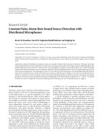
cells (see Figure 1) are considered. In Figure 3, the through-
put of the BE users based on the real SINR-rate mapping
and the approximation is shown over the average number of
active BE users. As can be observed, Algorithm 2 achieves up
to 30% more throughput compared to load-balancing. The

real and approximated rates match pretty well in the region
for low user request rates, but also at high load the deviation
is small compared to the gain. The sum utility per cell area
and the upper bound are shown in Figure 4. The utility gain
of Algorithm 2 compared to load-balancing is also almost as
large as of the throughput because of the low curvature of
ψ. The distance to the bound is of special interest; at high
call arrival rates the distance is almost zero, indicating that
Algorithm 2 performs close to optimum and no significant
gains could be achieved by using Algorithm 1 instead. At
lower rates this is different. Here, the dynamic procedure
pays the price for its simplicity in terms of performance loss.
The main reason for the loss results from the fluctuation of λ.
At low request rates a user’s call setup or service termination
has a great impact on the resource allocation of the other
users in the cell and therefore leads to strong variations of
λ over time. The fluctuation of λ directly influences the set
of optimum BSs M
opt
of users and therefore often leads to
the case that users find themselves assigned to a currently
nonoptimal BS. In this case, the dynamic algorithm looses
performance since the cell selection is only allowed once
per user in general. Higher utility values could be obtained
here by allowing users to perform intersystem hand-overs
so that each user would be assigned to M
opt
again. This
characteristic is also reflected in the looseness of the bound.
Unlike to low request rates, if the average number of users in

a cell is high the influence of a single-user arrival or departure
from a cell on λ is diminishing and a user’s optimum BS
hardly changes during the service time. In this case the
performance is almost optimal and the bound gets very tight.
The tightness also indicates that the influence of the users
pedestrian mobility and therefore the variation of
R (and on
M
opt
) is negligible in this scenario.
For the heterogeneous UMTS GSM/EDGE system the
following interpretation of the optimum assignment strategy
can be given. One observes that
R is a monotonically
increasing function of a user’s SINR for both air interfaces.
Therefore, for a given λ the optimum cell/RAT selection
70605040302010
Average number of best effort users per cell area
Algorithm 2
Load based
Algorithm 2 approximation
Load based approximation
1400
1600
1800
2000
2200
2400
2600
2800

Sum be throughput (kbit/sper cell area)
Figure 3: BE throughput with and without linear approximation
(9) without slow fading.
m
opt,i
= argmin
m
λ
m
/R
i,m
(β
i,m
) reduces to an SINR thresh-
old. This threshold depends on the air interface and the
service type through
R(β)andonλ which can be interpreted
as the load situation of the BS. The threshold characteristic
can be observed in Figure 5, where the BE user assignment
in terms of the selected RAT is shown by color shades;
Algorithm 2 assigns users to UMTS that are in the red
area close to the BSs and users in the blue area to GSM.
The border of both areas is characterized by the threshold
SINR of each RAT which has a lobe pattern because of the
directional antenna characteristics. The pattern looks very
regular in Figure 5 due to equal average loads in each cell
of an air interface (and therefore equal λ for BSs of one
RAT) and collocated sites of UMTS and GSM BSs. However,
Algorithm 2 will also flexibly adapt itself to the optimum
configuration in case of arbitrary, not necessary collocated,

BS positioning and varying load situations without any
change in configuration of the algorithm. The optimum area
patternwillthenofcourselookdifferent. Contrary to the BE
users Algorithm 2 will assign almost all voice users to UMTS
in the presented scenario. This is due to the fact that time-
slot sharing is not possible in GSM for voice users. Therefore,
the maximum slot rate of a voice user is much lower than
inUMTS.Thus,amuchlowerλ of the GSM BS compared
to the λ of the UMTS BS would be required to make GSM
attractive for an assignment. This instance might suggest that
also the major part of the gain of Algorithm 2 is based on the
low effectivity of voice in GSM, which is not avoided in load
balancing. Simulations however show that also for pure BE
traffic gains of more than 20% are obtained.
So far slow fading has not been active in the simulations
to demonstrate that the utility bound can be tight and to
visualize the assignment policy of Algorithm 2 qualitatively.
In Figure 6, the sum utility and the bound is shown for
the scenario above however this time with slow fading
EURASIP Journal on Wireless Communications and Networking 11
70605040302010
Average number of best effort users per cell area
Algorithm 2
Load based
Bound algorithm 2
4000
6000
8000
10000
12000

Sum utility (per cell area)
Figure 4: Sum utility U =

i∈I
b
ψ
i
(R
i
) and upper bound U + ΔL
without slow fading.
×10
3
3210−1−2−3
X coordinate (m)
UMTS
optimal
GSM
optimal
Transceiver position
−3000
−2000
−1000
0
1000
2000
3000
Y coordinate (m)
0
0.2

0.4
0.6
0.8
1
Figure 5: RAT assignment of BE users without slow fading: 1 →
100% assigned to UMTS 0 → 100% assigned to GSM.
corresponding to [14] in both air interfaces with a variance
of 6 dB. Considering load balancing, the slow fading does
hardly influence the performance. For Algorithm 2 however
the users’ mobility in connection with the slow fading has a
nonnegligible impact. Now, even small changes in position
can result in large channel gain and therefore
R differences
which lead to more wrongly assigned users and looseness
of the bound. Nevertheless, still a gain of approximately
20% is achieved. Similarly the performance of Algorithm 2
decreases and the bound gets less tight without slow fading
in case the velocity is increased. For completeness, it is
noted here that in case users do not change their position
the tightness of the bound under slow fading is similar to
Figure 4.
TheobservationsmadeinSection 3 and in the simula-
tions open up the way for even more simplified algorithms
that might be interesting for practical applications. For given
70605040302010
Average number of best effort users per cell area
Algorithm 2
Load based
Bound algorithm 2
4000

6000
8000
10000
12000
Sum utility (per cell area)
Figure 6: Sum utility and upper bound with slow fading 6 dB.
scenarios fixed base station weights λ or service dependent
SINR, channel or even distance thresholds could be applied
for the cell/RAT selection or as triggers for intersystem hand-
overs. Additionally, in case users are subject to strong channel
variations, for example, by mobility or fading during a
service request updating the cell/RAT selection and therefore
executing Algorithm 2(a) at more frequent intervals is an
option to improve the performance and get close to the
optimum again.
6. Conclusions
In this paper, we developed an optimization framework for
wireless heterogeneous multicell scenarios. Having derived
the feasible rate regions for air interfaces with orthogo-
nal resource assignment and a convex approximation for
interference limited radio access technologies we introduced
a convex utility maximization problem formulation for
heterogeneous scenarios. We gained general insights on
the problem solution and derived simple assignment rules
that lead to the global optimum by exploiting the dual
problem formulation. These observations were then used
to develop decentralized algorithms for static scenarios
and then simplified for dynamic settings. Although the
simplifications came at the cost of the optimality still high
gains in comparison to a simple load-balancing algorithm

were obtained and close to optimum performance could be
shown by simulations based on a duality bound.
Acknowledgment
The authors are supported in part by the Bundesministerium
f
¨
ur Bildung und Forschung (BMBF) under Grant FK 01 BU
566.
12 EURASIP Journal on Wireless Communications and Networking
References
[1] J. P
´
erez-Romero, O. Sallent, and R. Agust
´
ı, “On the optimum
traffic allocation in heterogeneous CDMA/TDMA networks,”
IEEE Transactions on Wireless Communications,vol.6,no.9,
pp. 3170–3174, 2007.
[2] A. Furusk
¨
ar and J. Zander, “Multiservice allocation for
multiaccess wireless systems,” IEEE Transactions on Wireless
Communications, vol. 4, no. 1, pp. 174–183, 2005.
[3] I. Blau and G. Wunder, “User allocation in multi-system,
multi-service scenarios: upper and lower performance bound
of polynomial time assignment algorithms,” in Proceedings of
the 41st Annual Conference on Information Sciences and Systems
(CISS ’07), pp. 41–46, Baltimore, Md, USA, March 2007.
[4] I. Blau, G. Wunder, I. Karla, and R. Siegle, “Cost based
heterogeneous access management in multi-service, multi-

system scenarios,” in Proceedings of the 18th IEEE Internat ional
Symposium on Personal, Indoor and Mobile Radio Communica-
tions (PIMRC ’07), pp. 1–5, Athens, Greece, September 2007.
[5] E. Stevens-Navarro, Y.Lin, and V.W. S. Wong, “An MDP-based
vertical handoff decision algorithm for heterogeneous wireless
networks,” IEEE Transactions on Vehicular Technology, vol. 57,
no. 2, pp. 1243–1254, 2008.
[6] J. Mo and J. Walrand, “Fair end-to-end window-based con-
gestion control,” IEEE/ACM Transactions on Networking, vol.
8, no. 5, pp. 556–567, 2000.
[7] S. Sta
´
nczak, M. Wiczanowski, and H. Boche, “Distributed
utility-based power control: objectives and algorithms,” IEEE
Transactions on Signal Processing, vol. 55, no. 10, pp. 5058–
5068, 2007.
[8] M. Chiang, “Balancing transport and physical layers in
wireless multihop networks: jointly optimal congestion con-
trol and power control,” IEEE Journal on Selected Areas in
Communications, vol. 23, no. 1, pp. 104–116, 2005.
[9] J. Huang, R. A. Berry, and M. L. Honig, “Distributed inter-
ference compensation for wireless networks,” IEEE Journal on
Selected Areas in Communications, vol. 24, no. 5, pp. 1074–
1084, 2006.
[10] A. Goldsmith, Wireless Communications, Cambridge Univer-
sity Press, New York, NY, USA, 2005.
[11] S. Boyd and L. Vandenberghe, Convex Optimization,Cam-
bridge University Press, New York, NY, USA, 2004.
[12] D. P. Bertsekas, Nonlinear Programming, Athena Scientific,
Belmont, Mass, USA, 2nd edition, 1995.

[13] S. Borst, A. Prouti
`
ere, and N. Hegde, “Capacity of wireless data
networks with intra- And inter-cell mobility,” in Proceedings
of the 25th IEEE International Conference on Computer Com-
munications (INFOCOM ’06), pp. 1–2, Barcelona, Spain, April
2006.
[14] ETSI, “Selection procedures for the choice of radio transmis-
sion,” Tech. Rep. 101 112 V3.1.0, UMTS, November 2001.
[15] ETSI, “Radio network planning aspects,” Tech. Rep. 101 362
V8.3.0, GSM, 1999.