Wave Propagation 2011 Part 3 pdf
Bạn đang xem bản rút gọn của tài liệu. Xem và tải ngay bản đầy đủ của tài liệu tại đây (671.86 KB, 30 trang )
Uniform Asymptotic Physical Optics Solutions for a Set of Diffraction Problems
49
in which
2
k is the propagation constant in the double-negative metamaterial,
2
θ is the
negative refraction angle, and
j
ii
j
ij
j
ii
j
kcos kcos
R
k cos k cos
θ
−θ
=
θ
+θ
ii
jj
ij
ii
jj
k cos k cos
R
k cos k cos
⊥
θ
−θ
=
θ
+θ
(61)
ij
ii
j
ii
j
2k cos
T
kcos kcos
θ
=
θ
+θ
ij
ii
ii
jj
2k cos
T
kcos kcos
⊥
θ
=
θ
+θ
(62)
In (61) and (62),
130
kkk
=
= ,
13
θ
=θ and the superscripts i and j refer to the left and right
media involved in the propagation mechanism.
Comparisons with COMSOL MULTIPHYSICS
®
results are reported in Figs. 14 and 15 with
reference to
'45φ= °
. As can be seen, the UAPO diffracted field guarantees the continuity of
the total field across the two discontinuities of the GO field in correspondence of the
incidence and reflection shadow boundaries, and a very good agreement is attained.
Accordingly, the accuracy of the UAPO-based approach is well assessed also in the case of a
lossless double-negative metamaterial layer.
3.3 Anisotropic impedance layer
A layer characterised by anisotropic impedance boundary conditions on the illuminated
face is now considered. Such conditions are represented by an impedance tensor
x' z'
ˆˆ
ˆˆ
Z Z x'x' Z z'z'=+ having components along the two mutually orthogonal principal axes
of anisotropy
ˆ
x'
and
ˆ
z'
. The structure is opaque so that the transmission matrix does not
exist and, according to (Gennarelli et al., 1999), the elements of
R can be so expressed:
Fig. 14. Amplitude of E
β
if
β
=
i
'
E1,
φ
=
i
'
E0 and '90
β
=°, ' 45
φ
=°. Circular path with
0
5ρ= λ . Layer characterised by
r
4
ε
=− ,
r
1
μ
=− and
0
d0.125
=
λ .
Wave Propagation in Materials for Modern Applications
50
Fig. 15. Amplitude of E
φ
if
β
=
i
'
E0,
φ
=
i
'
E1 and '90
β
=°, ' 45
φ
=°. Circular path with
0
5ρ= λ
. Layer characterised by
r
4
ε
=−
,
r
1
μ
=−
and
0
d0.125
=
λ
.
(
)
(
)
2i 2i
11
2i 2i
A1ACBcos Ccos
R
A1ACBcos Ccos
−
++ + θ− θ
=
+
−− θ− θ
(63)
()
θ
=− =
+
−− θ− θ
i
12 21
2i 2i
2B cos
RR
A 1 AC B cos C cos
(64)
(
)
(
)
2i 2i
22
2i 2i
A1ACBcos Ccos
R
A1ACBcos Ccos
+
++ θ+ θ
=−
+
−− θ− θ
(65)
in which, if
χ is the angle between
ˆ
x'
and
ˆ
e
⊥
,
=
χ+ χ
ζζ
22
x'
z'
00
Z
Z
A sin cos (66)
()
=
−χχ
ζ
x' z'
0
1
B Z Z sin cos (67)
⎡
⎤
=
−χ+χ
⎢
⎥
ζζ
⎣
⎦
22
x'
z'
00
Z
Z
C cos sin (68)
Uniform Asymptotic Physical Optics Solutions for a Set of Diffraction Problems
51
If an isotropic impedance boundary condition is considered (i.,e., the principal axes of
anisotropy does not exist and
=
=
x' z'
ZZZ),
=
=
12 21
RR0, whereas
11
R and
22
R reduce to
the standard reflection coefficients for parallel and perpendicular polarisations.
If the illuminated surface is perfectly electrically conducting, the out diagonal elements are
again equal to zero, whereas
=
11
R1 and
=
−
22
R1 since
=
=
x' z'
ZZ0.
Fig. 16. Amplitude of E
β
if
β
=
i
'
E1,
φ
=
i
'
E0 and '90
β
=°, ' 60
φ
=°. Circular path with
0
5ρ= λ . Layer characterised by
0
Z
j
0.5
ζ
= .
Fig. 17. Amplitude of E
β
if
β
=
i
'
E1,
φ
=
i
'
E0 and '90
β
=°, ' 60
φ
=°. Circular path with
0
5ρ= λ . Layer characterised by
0
Z
j
0.5ζ= .
Wave Propagation in Materials for Modern Applications
52
The magnitudes of the electric field
β
–components of the GO field and the UAPO diffracted
field on a circular path with
ρ
=λ
0
5 are considered in Fig. 16, where also the diffracted
field obtained by using the Maliuzhinets solution (Bucci & Franceschetti, 1976) is reported in
the case of an isotropic impedance boundary condition. A very good agreement exists
between the two diffracted fields. The accuracy of the UAPO-based approach is further
confirmed by comparing the total fields shown in Fig. 17, where also the COMSOL
MULTIPHYSICS
®
results are shown.
4. Junctions of layers
The UAPO solution for the field diffracted by the edge of a truncated planar layer as derived
in Section 2 can be extended to junctions by taking into account the diffraction contributions
of the layers separately. This very useful characteristic is due to the property of linearity of
the PO radiation integral. Accordingly, if the junction of two illuminated semi-infinite layers
as depicted in Fig. 18 is considered, the total scattered field in (1) can be so rewritten:
+
⎡⎤
=− − ζ + × =
⎣⎦
⎡⎤
=− − ζ + × +
⎢⎥
⎣⎦
⎡⎤
−−ζ+× =+
⎢⎥
⎣⎦
∫∫
∫∫
∫∫
12
11
1
22
2
sPOPO
00
sms
SS
PO PO
00 1
sms
S
PO PO s s
00 2
sms
12
S
ˆˆ ˆ
Ejk (IRR)JJRG(r,r')dS
ˆˆ ˆ
jk (I RR) J J R G(r,r') dS
ˆˆ ˆ
j
k(IRR)JJ RG(r,r')dSEE
(69)
and then
=+
12
DD D, with
1
D given by (46). The diffraction matrix
2
D related to the
wave phenomenon originated by the edge of the second layer forming the junction can be
determined by using again the methodology described in Section 2. If the external angle of
the junction is equal to
n
π
, a
(
)
n1
−
π
rotation of the edge-fixed coordinate system must be
considered for the second layer. The incidence and observation angles with respect to the
illuminated face are now equal to n '
π
−φ and n
π
−φ, respectively, so that the UAPO
solution for
2
D uses n '
π
−φ instead of '
φ
and n
π
−φ instead of
φ
. The results reported in
(Gennarelli et al., 2000) with reference to an incidence direction normal to the junction of
two resistive layers confirm the validity of the approach and, in particular, the accuracy of
the solution is well assessed by resorting to a numerical technique based on the Boundary
Element Method (BEM).
S
f
'
(f =
np)
2
f
x
y
S
(f =
np)
2
P
r
(f=0)
S
1
Fig. 18. Junction of two planar truncated layers.
Uniform Asymptotic Physical Optics Solutions for a Set of Diffraction Problems
53
5. Conclusions and future activities
UAPO solutions have been presented for a set of diffraction problems originated by plane
waves impinging on edges in penetrable or opaque planar thin layers. The corresponding
diffracted field has been obtained by modelling the structure as a canonical half-plane and
by performing a uniform asymptotic evaluation of the radiation integral modified by the PO
approximation of the involved electric and magnetic surface currents. The resulting
expression is given terms of the UTD transition function and the GO response of the
structure accounting for its geometric, electric and magnetic characteristics. Accordingly, the
UAPO solution possesses the same ease of handling of other solutions derived in the UTD
framework and has the inherent advantage of providing the diffraction coefficients from the
knowledge of the reflection and transmission coefficients. It allows one to compensate the
discontinuities in the GO field at the incidence and reflection shadow boundaries, and its
accuracy has been proved by making comparisons with purely numerical techniques. In
addition, the time domain counterpart can be determined by applying the approach
proposed in (Veruttipong, 1990), and the UAPO solution for the field diffracted by junctions
can be easily obtained by considering the diffraction contributions of the layers separately.
To sum up, it is possible to claim that UAPO solutions are very appealing from the
engineering standpoint.
Diffraction by opaque wedges has been considered in (Gennarelli et al., 2001; Gennarelli &
Riccio, 2009b). By working in this context, the next step in the future research activities may
be devoted to find the UAPO solution for the field diffracted by penetrable wedges (f.i.,
dielectric wedges).
6. Acknowledgment
The author wishes to thank Claudio Gennarelli for his encouragement and helpful advice as
well as Gianluca Gennarelli for his assistance.
7. References
Burnside, W.D. & Burgener, K.W. (1983). High Frequency Scattering by a Thin Lossless
Dielectric Slab.
IEEE Transactions on Antennas and Propagation, Vol. AP-31, No. 1,
January 1983, 104-110, ISSN: 0018-926X.
Balanis, C.A. (1989).
Advanced Engineering Electromagnetics, John Wiley & Sons, ISBN: 0-471-
62194-3, New York.
Bucci, O.M. & Franceschetti, G. (1976). Electromagnetic Scattering by a Half-Plane with Two
Face Impedances,
Radio Science, Vol. 11, No. 1, January 1976, 49-59, ISSN: 0048-6604.
Clemmow, P.C. (1950). Some Extensions of the Method of Integration by Steepest Descent.
Quarterly Journal of Mechanics and Applied Mathematics, Vol. 3, No. 2, 1950, 241-256,
ISSN: 0033-5614.
Clemmow, P.C. (1996).
The Plane Wave Spectrum Representation of Electromagnetic Fields,
Oxford University Press, ISBN: 0-7803-3411-6, Oxford.
Ferrara, F.; Gennarelli, C.; Pelosi, G. & Riccio, G. (2007a). TD-UAPO Solution for the Field
Diffracted by a Junction of Two Highly Conducting Dielectric Slabs.
Electromagnetics, Vol. 27, No. 1, January 2007, 1-7, ISSN: 0272-6343.
Wave Propagation in Materials for Modern Applications
54
Ferrara, F.; Gennarelli, C.; Gennarelli, G.; Migliozzi, M. & Riccio, G. (2007b). Scattering by
Truncated Lossy Layers: a UAPO Based Approach. Electromagnetics, Vol. 27, No. 7,
September 2007, 443-456, ISSN: 0272-6343.
Gennarelli, C.; Pelosi, G.; Pochini; C. & Riccio, G. (1999). Uniform Asymptotic PO Diffraction
Coefficients for an Anisotropic Impedance Half-Plane.
Journal of Electromagnetic
Waves and Applications
, Vol. 13, No. 7, July 1999, 963-980, ISSN: 0920-5071.
Gennarelli, C.; Pelosi, G.; Riccio, G. & Toso, G., (2000). Electromagnetic Scattering by
Nonplanar Junctions of Resistive Sheets.
IEEE Transactions on Antennas and
Propagation
, Vol. 48, No. 4, April 2000, 574-580, ISSN: 0018-926X.
Gennarelli, C.; Pelosi, G. & Riccio, G. (2001). Approximate Diffraction Coefficients of an
Anisotropic Impedance Wedge.
Electromagnetics, Vol. 21, No. 2, February 2001, 165-
180, ISSN: 0272-6343.
Gennarelli, G. & Riccio, G. (2009a). A UAPO-Based Solution for the Scattering by a Lossless
Double-Negative Metamaterial Slab.
Progress In Electromagnetics Research M, Vol. 8,
2009, 207-220, ISSN: 1937-8726.
Gennarelli, G. & Riccio, G. (2009b).
Progress In Electromagnetics Research B, Vol. 17, 2009, 101-
116, ISSN: 1937-6472.
Keller, J.B. (1962). Geometrical Theory of Diffraction.
Journal of Optical Society of America, Vol.
52, No. 2, February 1962, 116-130, ISSN: 0030-3941.
Kouyoumjian, R.G. & Pathak, P.H. (1974). A Uniform Geometrical Theory of Diffraction for
an Edge in a Perfectly Conducting Surface.
Proceedings of the IEEE, Vol. 62, No. 11,
November 1974, 1448-1461, ISSN: 0018-9219.
Luebbers, R.J. (1984). Finite Conductivity Uniform UTD versus Knife Diffraction Prediction
of Propagation Path Loss.
IEEE Transactions on Antennas and Propagation, Vol. AP-
32, No. 1, January 1984, 70-76, ISSN: 0018-926X.
Maliuzhinets, G.D. (1958). Inversion Formula for the Sommerfeld Integral.
Soviet Physics
Doklady, Vol. 3, 1958, 52-56.
Senior, T.B.A. & Volakis, J.L. (1995).
Approximate Boundary Conditions In Electromagnetics. The
Institution of Electrical Engineers, ISBN: 0-85296-849-3, Stevenage.
Veruttipong, T.W. (1990). Time Domain Version of the Uniform GTD.
IEEE Transactions on
Antennas and Propagation
, Vol. 38, No. 11, November 1990, 1757-1764, ISSN: 0018-
926X.
3
Differential Electromagnetic Forms
in Rotating Frames
Pierre Hillion
Institut Henri Poincaré, 86 Bis Route de Croissy, 78110 Le Vésinet,
France
1. Introduction
Differential forms are completely antisymmetric homogeneous r-tensors on a differentiable
n-manifold 0 ≤ r ≤ n belonging to the Grasssman algebra [1] and endowed by Cartan [2]
with an exterior calculus. These differential forms found an immediate application in
geometry and mechanics; introduced by Deschamps [3,4] in electromagnetism, they have
known in parallel with the expansion of computers, an increasing interest [5-9] because
Maxwell’s equations and the constitutive relations are put in a manifestly independent
coordinate form.
In the Newton (3+1) space-time, with the euclidean metric ds
2
= dx
2
+ dy
2
+ dz
2
the
conventional Maxwell equations in which the E, B, D, H fields are 3-vectors have, in absence
of charge and current, the Gibbs representation
∇.B = 0, ∇∧Ε + 1/c∂
t
B = 0 (1a)
∇.D = 0, ∇∧H − 1/c∂
t
D = 0 (1b)
and, they also have the differential form representation (∂
τ
=1/c∂
t
) [5,7]
d ∧ E +∂
τ
B = 0, d ∧ B = 0 (2a)
d ∧ H − ∂
τ
D = 0, d ∧ D = 0 (2b)
d = dx∂
x
+ dy∂
y
+dz∂
z
is the exterior derivative, E , H the differential 1-forms
E = E
x
dx + E
y
dy + E
z
dz, H = H
x
dx + H
y
dy + H
z
dz (3a)
and B , D the differential 2-forms
B = B
x
(dy∧dz) + B
y
(dz∧dx) +B
z
(dx∧dy) , D = −[ D
x
(dy∧dz) + D
y
(dz∧dx) +D
z
(dx∧dy)] (3b)
We are interested here, for reasons to be discussed in Sec.(6) in a Frenet-Serret frame
rotating around oz with a constant angular velocity requiring a relativistic processing, We
shall prove that this situation leads to an Einstein space-time with a riemannian metric. As
an introduction to this problem, we give a succcinct presentation of differential
electromagnetic forms in a Minkowski space-time with the metric ds
2
= dx
2
+ dy
2
+
dz
2
−c
−2
∂
t
2
.
Wave Propagation in Materials for Modern Applications
56
2. Differential forms in Minkowski space-time [7]
In absence of charge and current, the Maxwell equations have the tensor representaation [10,
11]
∂
σ
F
μν
+∂
μ
F
νσ
+ ∂
ν
F
σμ
= 0 a) ∂
ν
F
μν
= 0 b) (4)
the greek (resp.latin) indices take the values 1,2,3,4 (resp.1,2,3) with x
1
= x, x
2
= y, x
3
= z, x
4
=
ct, ∂
j =
∂/∂x
j
, ∂
4 =
1/c∂/∂
t
and the summation convention is used. The components of the ten-
sors F
μν
and F
μν
are with the 3D Levi-Civita tensor ε
ijk
B
i
= ½ ε
ijk
F
jk
, E
i
= − F
i4
, H
i
= ½ ε
ijk
F
jk
, D
i
= − F
i4
(5)
and in vacuum
D = ε
0
E, H = µ
0
−1
B , (ε
0
μ
0
)
1/2
= 1/c (5a)
Let d be the exterior derivative operator
d = (∂
x
dx +∂
y
dy +∂
z
dz +∂
t
dt )∧ (6)
and F =E + B be the two-form in which :
E = E
x
(dx∧cdt) + E
y
(dy∧cdt) + E
z
(dz∧cdt)
B = B
x
(dy∧dz) + B
y
(dz∧dx) + B
z
(dx∧dy) (7)
Then the Maxwell equations (4a) have the differential 3-form representation d F = 0.
Similarly for G =D + H with :
H = H
x
(dx∧cdt) + H
y
(dy∧cdt) + H
z
(dz∧cdt)
D = −[D
x
(dy∧dz) + D
y
(dz∧dx) + D
z
(dx∧dy)] (8)
the differential 3-form representation of Maxwell’s equations (4b) is d G = 0.
To manage the constituive relations (5a) the Hodge star operator [6,9] is introduced
* (dx∧cdt) = c
−1
(dy∧dz) , * (dy∧dz) = c (dx∧cdt)
* (dy∧cdt) = c
−1
(dz∧dx) , * (dz∧dx) = c (dy∧cdt)
* (dz∧cdt) = c
−1
(dx∧dy) , * (dx∧dy) = c (dz∧cdt) (9)
Applying the Hodge star operator to F gives *F = *E + *B and one checks easily the re-
lation G = λ
0
*F with λ
0
=(ε
0
/μ
0
)
1/2
so that the Maxwell equations in the Minkowski vacu-
um, have the diffrerential 3-form representation
dF = 0, d *F = 0 (10)
3. Electromagnetidsm in a Frenet-Serret rotating frame
We consider a frame rotating with a constant angular velocity Ω around oz. Then, using the
Trocheris-Takeno relativistic description of rotation [12, 13], the relations between the
Differential Electromagnetic Forms in Rotating Frames
57
cylindrical coordinates R,Φ,Z,T and r,φ,z,t in the natural (fixed) and rotating frames are
with ß = ΩR /c
R= r, Φ = φ coshβ − ct/r sinhβ
Z = z , cT = ct coshβ − rφ sinhβ (11)
and a simple calculation gives the metric ds
2
in the rotating frame
ds
2
= c
2
dt
2
− dz
2
− r
2
dφ
2
− (1+B
2
−A
2
) dr
2
− 2(A sinhß + B coshß) cdt dr −
2(A coshß + B sinhß) r dr dφ (12)
A = ß sinhß ct/r + ß coshß φ + sinhß φ, B = ß sinhß φ +ß coshß ct/r − sinhß ct/r (12a)
Using the notations x
4
= ct, x
3
= z, x
2
= φ, x
1
= r, we get from (12) ds
2
= g
μν
dx
μ
dx
ν
with
g
44
= 1, g
33
= −1, g
22
= −r
2
, g
11
= −(1+ B
2
−A
2
)
g
14
= g
41
= 2(A sinhß + B coshß), g
12
= g
21
= 2(A coshß + B sinhß) (13)
The determinant g of g
μν
is
g = g
33
[ g
11
g
22
g
44
− g
12
2
g
44
− g
14
2
g
22
]
= R [g
11
− g
12
2
r
−2
− g
14
2
] (14)
but
g
12
2
r
−2
+ g
14
2
= 4(A
2
− B
2
) (14a)
and, taking into account the expression (13) of g
11
, we get finally
g = r
2
[5(A
2
−B
2
) − 1], A
2
−B
2
= (φ
2
− c
2
t
2
/r
2
)(ß
2
+ sinh
2
ß + 2ß sinhß coshß) (15)
So, the rotating Frenet-Serret frame defines an Einstein space-time with the riemannian
metric ds
2
= g
μν
dx
μ
dx
ν
, and in this Einstein space-time the Maxwell equations have the
tensor representation[14, 15]
∂
σ
G
μν
+∂
μ
G
νσ
+ ∂
ν
G
σμ
= 0 a) ∂
ν
(|g|
1/2
G
μν
) = 0 b) (16)
in which, using the cylindrical coordinates r,φ.z ,t with x
1
= r, x
2
= φ, x
3
= z, x
4
= ct ; ∂
1
= ∂
r
,
∂
2
= ∂
φ
, ∂
3
= ∂
z
, ∂
4
=1/c ∂
t
, the components of the electromagnetic tensors are
G
12
= rB
z
, G
13
= −Β
φ
, G
23
= rB
r
; G
14
=−E
z
, G
24
= −rE
φ
, G
34
= −E
z
G
12
=H
z
/r, G
13
= −H
φ
, G
23
= H
r
/r; G
14
D
z
, G
2
4
= D
φ
/r, G
34
= D
z
(17)
To work with the differential forms, we introduce the exterior derivative
d
= (∂
r
dr+∂
φ
dφ+∂
z
dz+∂
t
dt) ∧ (18)
(underlined expressions mean that they are defined with the cylindrical coordinates r, φ,z,t)
and the two-forms F =E + B with
Wave Propagation in Materials for Modern Applications
58
E
= E
r
(dr∧cdt) + E
φ
(rdφ∧cdt) + E
z
(dz∧cdt)
B
= B
r
(rdφ∧dz) + B
φ
(dz∧dr) + B
z
(dr∧rdφ) (19a)
and writing |g|
1/2
= rq, q = [5(A
2
-B
2
)-1]
1/2
the two-form G =D + H
D
=− q [D
r
(rdφ∧dz) + D
φ
(dz∧dr) + D
z
(dr∧rdφ)]
H
= q[H
r
(dr∧cdt) + H
φ
(rdφ∧cdt) + H
z
(dz∧cdt)] (19b)
Then, the Maxwell equatios have the 3-form representation
dF = 0 , d G = 0 (20)
A simple calculation gives
d F
= [(∂
r
(rB
r
) +∂
φ
B
φ
+∂
z
(rB
z
)] (dr∧ dφ∧ dz) +
[∂
t
(rΒ
r
) + c{∂
φ
Ε
z
−∂
z
(rΕ
φ
)}] (dφ∧ dz∧ dt) +
[∂
t
Β
φ
+ c(∂
z
Ε
r
−∂
r
Ε
z
)] (dz∧ dr∧ dt) +
[∂
t
(rΒ
z
)+ c{∂
r
(rΕ
φ
)−∂
φ
Ε
r
}] (dr∧ dφ∧ dt) (21a)
dG
= − [∂
r
(qrD
r
) +∂
φ
(qD
φ
) +∂
z
(qD
z
)] (dr∧ dφ∧ dz) +
[−∂
t
(qrD
r
) + c {∂
φ
(qH
z
) −∂
z
(qrH
φ
)}] (dφ∧ dz∧ dt) +
[−∂
t
(qD
φ
) + c {∂
z
(qH
r
) −∂
r
(qH
z
)}] (dz∧ dr∧ dt) +
[−∂
t
(qrD
z
) + c {∂
r
(qrH
φ
−∂
φ
(qH
r
)}] (dr∧ dφ∧ dt) (21b)
The Hodge star operator needed to take into account the constitutive relations (5a) in
vacuum is defined by the relation
* (dr∧cdt) = −qc
−1
(rdφ∧dz), * (rdφ∧dz) = q
−1
c (dr∧cdt)
* (rdφ∧cdt) = −qc
−1
(dz∧dr) , * (dz∧dr) = q
−1
c (rdφ∧cdt)
* (dz∧cdt) = −qc
−1
(dr∧rdφ), * (dr∧rdφ) = q
−1
c (dz∧cdt) (22)
Applying (22) to F
gives *F = *E + *B and it is easily checked that G = λ
0
*F with
λ
0
=(ε
0
/μ
0
)
1/2
so that in vacuum dF = 0 , d *F = 0.
4. Wave equations in vacuum
4.1 Minkowski space-time
The wave equations satisfied by the electromagnetic field (in absence of charges and cur-
rents) are obtained from differential forms with the help of the Laplace-De Rham operator
[6,8]
L = (d* d* + * d* d)∧ (23)
Differential Electromagnetic Forms in Rotating Frames
59
requiring the Hodge star operators for the n-forms, n = 1,2,3. They are given in Appendix A
where, using the exterior derivative (6), and assuming E
x
= E
y
= 0 so that the two-form (7)
becomes E
z
= E
z
(dz∧cdt), we get
L E
z
= (∆−c
-2
∂
t
2
) E
z
(dz∧cdt), ∆ = ∂
x
2
+∂
y
2
+∂
z
2
(24)
A similar relation exists for E
x,
E
y
and for the components of the B-field so that, we get
finally for the 2-form F:
L F = (∆−c
-2
∂
t
2
) F
μν
(dx
μ
∧dx
ν
) (25)
so that the wave equation has the 2-form representation L F = 0 .
4.2 Einstein space-time
4.2.1 Cartesian frame
In a riemannian cartesian frame, the components of the electromagnetic field tensor ·F
μν
are
solutions of the tensor wave equation [16]
g
αβ
∇
α
∇
β
F
μν
− 2R
μναρ
F
ρα
+ R
μ
ρ
F
ρν
− R
ν
ρ
F
ρμ
= 0 (26)
∇
α
is the covariant derivative, R
μναρ
and R
μ
ρ
the Riemann curvature and Ricci tensors
defined in terms of Christtoffel symbols Γ
α,βμ
,
Γ
ρ
αμ
Γ
β,μν
= ½ (∂
ν
g
βμ
+ ∂
μ
g
βν
− ∂
β
g
μν
), Γ
α
μν
= g
αβ
Γ
β,μν
(27)
by the relations in which ∂
1
= ∂
x
, ∂
2
= ∂
y
, ∂
3
= ∂
y
, ∂
4
= 1/c∂
t
,
R
αβμν
= ∂
ν
Γ
α,βμ
−∂
μ
Γ
α.βν
+ Γ
ρ
αμ
Γ
ρ,βν
− Γ
ρ
αν
Γ
ρ,βμ
R
αβ
μν
= g
αρ
g
βσ
R
ρσμν
, R
μ
ν
= R
να
αμ
. (28)
Now, it is proved [6] that the Laplace-De Rham operator L = d*d* + *d*d applied to the two
form (7) written
E =F
14
(dx
1
∧dx
4
) + F
24
(dx
2
∧dx
4
) + F
34
(dx
3
∧dx
4
) (29)
in which dx
1
= dx, dx
2
= dy, dx
3
= dz, dx
4
= cdt gives for the component F
i4
L E = ½(g
αβ
∇
α
∇
β
F
i4
− 2R
i4
αρ
F
ρα
+ R
i
ρ
F
ρ
4
− R
4
ρ
F
ρ
i
)( (dx
i
∧dx
4
) (30)
L E = 0 gives the 2-form representation of the wave equation in the Einstein space-time with
cartesian coordinates
A similar result is obtained for B writing −1/2F
ij
(dx
i
∧dx
j
) the B magnetic two-form (7) so
that
LB = −1/4(g
αβ
∇
α
∇
β
F
ij
− 2R
ij
αρ
F
ρα
+ R
i
ρ
F
ρ
j
− R
j
ρ
F
ρ
i
) (dx
i
∧dx
j
) (30a)
Summing (30) and (30a) gives
LF = ½ [g
αβ
∇
α
∇
β
F
μν
− 2R
μναρ
F
ρα
+ R
μ
ρ
F
ρν
− R
ν
ρ
F
ρμ
] (dx
μ
∧dx
ν
) (31)
In the Minkowski cartesian frame where g
ij
= δ
ij
, g
44
= −1, Eq.(31) reduces to (25).
Wave Propagation in Materials for Modern Applications
60
4.2.2 Frenet-Serret frame
In the Frenet-Serret frame, the Laplace-De Rham operator is defined with the exterior deri-
vative operator (18) and to get a relation such as (30) on the components of the electric field
requires some care. First with the greek indices associated to the polar coordinates as
previously, one has first to get the Christoffel symbols needed to define the covariant
derivative and according to (28), the Riemann curvature and Ricci tensors, a job performed
in Appendix B, we are now in position to transpose (30) to a rotating cyindrical frame. To
this end, the electric two-form (19a) with
dx
1
∧dx
4
= dr∧cdt, dx
2
∧dx
4
= dφ∧cdt, dx
3
∧dx
4
= dz∧cdt (32)
is written
E
= E
r
(dx
1
∧dx
4
) + rE
φ
(dx
2
∧dx
4
) + E
z
(dx
3
∧dx
4
) (33)
but E
r
, rE
φ
, E
z
are the G
i4
components of the G
μν
tensor (17) so that
leaving aside a minus sign
E = G
14
(dx
1
∧dx
4
) + G
24
(dx
2
∧dx
4
) + G
34
(dx
3
∧dx
4
) (34)
and we get
L E
= ½( (g
αβ
∇
α
∇
β
G
i4
− 2R
i4
αρ
G
ρα
+ R
i
ρ
G
ρ
4
− R
4
ρ
G
ρ
i
)) (dx
i
∧dx
4
) (35)
so that the components of the electric field are solutions of the two-form equation L E
= 0 in
the Frenet-Serret rotating frame. For the other components of the electromagnetic field, it
comes
L F
= ½( (g
αβ
∇
α
∇
β
G
μν
− 2R
μναρ
G
ρα
+ R
μ
ρ
G
ρν
− R
ν
ρ
G
ρμ
) (dx
μ
∧dx
ν
) (36)
We have only considered the two-form F because in vacuum G =λ
0
* F .
5. To solve differential form equations
The local 2-form representation (2) of Maxwell’s equations follows, as a consequence of the
Stokes’s theorem, from the Maxwell-Ampère and Maxwell-Faraday integral relations. Then,
coming back to these theorems, to solve differential form equations is tantamount to
perform the integrals
I = ∫
M
ω (37)
in which ω is a n-form, for instance F ou G, and M an oriented manifold with the same n-
dimension as the degree of the ω form [5].
In the 3D-space, the numerical evaluation of (37) is based on the finite element technique,
largely used [17, 18] in the simulation of partial differential equations. The manifold M is
described by a chain of simplexes made for instance of triangular surfaces, tetrahedral vo-
lumes… on which the Whitney forms [5,19,20] gives a manageable description of the n-
form ω. A simple example may be found in [19] and a through discussion of the technique in
[20]. These solutions may be called weak in opposition to the strong solutions of the
Maxwell’s equations (1).
Differential Electromagnetic Forms in Rotating Frames
61
The numerical process just described is limited to the 3D-space but in the 4D space-time, in
particular for the Frenet-Serret frame, ω depends on dt so that M has to be defined in terms
of 2-cells, 3-cells, 4-cells of space-time [21] and the Whitney forms must be generalized ac-
cordingly. It does not seem that computational works have been made in this domain.
6. Discussion
Differential electromagnetic forms are usually managed in a Newton space and more rarely
in a Minkowski space-time although, in this case, the comparison between tensors and diffe-
rential forms is very enlightning [7]. This formalism is analyzed here in an Einstein space-
time with a Riemann metric, particularly that of a Frenet-Serret frame. From a theoretical
point of view, except for some more intricate relations due to Riemann, Ricci tensors and
Christoffel symbols there is no difficulty to go from Newton to Einstein differential forms
The situation is different from a computational point of view, since as mentionned in Sec.5,
an important worrk has still to be performed to get the solutions of the differential form
equation in an Einstein space-time.
This work may be considered as a first step in a complete analysis of electromagnetic
differential forms in an Einstein space-time. The subjects to be discussed go from the
presence of charges and currents (left aside here) to boundary conditions with between the
introduction of potentials, the energy conveyed by the electromagnetic field and so on. This
extension could be performed in the syle used in [7] to analyze the electromagnetic
differential forms in a Minkowski space-time. In addition, it would make possible an
interesting comparison (al-ready sketched in Sec.4.1) with the electromagnetic tensor
formalism of the General Relati-vity [15].
Now, why to take an interest in rotating frames? A first response could have been ‘’Univer-
se’’ assumed cylindrical. But, although Einstein and Romer (also Levi Civita) have obtained
some exact cylindrical wave solutions of the general relativity equations [22], this cosmos
has been superseded by a spherical world (nevertheless, because of its particular properties,
some works are still devoted to the Levi Civita world [23]. A second response comes from
the analysis of the Wilsons’ experiments in which was measured the electric potential
between the inner and outer surfaces of a cylinder rotating in an external axially directed
magnetic field: an analysis with many different approaches [6,23,24,25] (the Trocheris-
Takeno des-cription of rotations is used in [25]). Finally, a third response is provided by the
increasing at-tention paid to paraxial optical beams with an helicoidal geometrical structure
[26], [27] lea-ding to a discussion of light propagation in rotating media: a problem object of
some dispu-tes [28-32].The relativistic theory of geometrical optics [15] is still a challenge to
which it would be interesting to see what could be the differential form contribution.
Appendix A: Minkowski space-time in vacuum
The four dimensional Hodge operator for Minkowski space-time is defined as follows [8]:
zero-forms and four-forms
* (dx∧ dy∧ dz ∧cdt) = −1, *1 = (dx∧ dy∧ dz ∧cdt) (A.1)
one-forms and three-forms
Wave Propagation in Materials for Modern Applications
62
* (dx∧ dy∧ dz ) = −cdt), * c dt = −(dx∧ dy∧ dz )
*(dy∧ dz∧ cdt ) = −dx, *dx = − (cdt∧ dy∧ dz )
*(dz∧ dx∧ cdt ) = −dy, *dy = − (cdt∧ dz∧ dx )
*(dx∧ dy∧ cdt ) = −dz, *dz = − (cdt∧ dx∧ dy ) (A.2)
two forms
*(dy∧dz) = − (dx∧cdt), *(dx∧cdt) = (dy∧dz)
*(dz∧dx) = − (dy∧cdt), *(dy∧cdt) = (dz∧dx)
*(dx∧dy) = − (dz∧cdt) , *(dz∧cdt) = (dx∧dy) (A.3)
Let us assume E
x
= E
y
= 0, then the electric two-form (7) becomes
E = E
z
(dz∧cdt) (A.4)
Applying the exterior derivative operator (6) to (B.4) and using (B.2) give
*d E = ∂
x
Ε
z
∧dy − ∂
y
Ε
z
∧dx (A.5)
and
d*d E = ∂
x
2
Ε
z
(dx∧dy) + ∂
z
∂
x
Ε
z
(dz∧dy) + ∂
t
∂
x
Ε
z
(dt∧dy) +
−[∂
y
2
Ε
z
(dy∧dx) + ∂
z
∂
y
Ε
z
(dz∧dx) + ∂
t
∂
y
Ε
z
(dt∧dx)] (A.6)
so that according to (A.3)
*d*d E = − ∂
z
2
Ε
z
(dz∧cdt) + ∂
z
∂
x
Ε
z
(dx∧cdt) −1/c∂
t
∂
x
Ε
z
(dz∧dx) +
−[∂
y
2
Ε
z
(dz∧cdt) − ∂
z
∂
y
Ε
z
(dy∧cdt) −1/ c∂
t
∂
y
Ε
z
(dy∧dz)] (A.7)
1ow, using (A.3) and (A.2), we also have
*d *E = −∂
z
Ε
z
∧cdt − ∂
t
Ε
z
∧dz (A.8)
and
d*d *E = −∂
z
∂
x
Ε
z
(dx∧cdt) − ∂
z
∂
y
Ε
z
(dy∧cdt) − ∂
z
2
Ε
z
(dz∧cdt) +
− 1/c [∂
t
2
Ε
z
(dt∧dz) +∂
t
∂
x
Ε
z
(dx∧dz) + ∂
t
∂
y
Ε
z
(dy∧dz)] (A.9)
Summing (A.7) and (A.9) gives
(*d*d + d*d *)E = − (∂
x
2
+∂
y
2
+∂
z
2
−c
−2
∂
t
2
) E
z
(dz∧cdt) (A.10)
Appendix B: Christoffel symbols
The Christoffel symbols are defined in terms of the g
μν
’s by the well known relations [14-16]
Γ
β,μν
= ½ (∂
ν
g
βμ
+ ∂
μ
g
βν
− ∂
β
g
μν
), Γ
α
μν
= g
αβ
Γ
β,μν
(B.1)
Differential Electromagnetic Forms in Rotating Frames
63
In these expressions, the greek indices take the values 1,2,3,4 corresponding in a cylindrical
frame to the coordinates x
1
= r, x
2
= φ, x
3
= z, x
4
= ct, while ∂
1
= ∂
r
, ∂
2
= 1/r ∂
φ
, ∂
3
= ∂
z
, ∂
4
= 1/c
∂
t
.
The relations (13) give the components g
μν
of the metric tensor for a Frenet-Serret rotating
frame and :
g
44
= 1, g
33
= −1, g
22
= −r
2
, g
11
= u(r,φ,t) , g
12
= g
21
= v(r,φ,t) , g
14
= g
41
= w(r,φ,t) (B.2)
the explicit expressions of the functions u,v,w are to be found in (13), no g
μν
depends on z.
Then, the non-null components of the Christoffel symbols are given for μ ≤ ν (because of the
μν-symmetry)
Γ
1,11
= ½ ∂
r
u , Γ
1,12
= ½ ∂
φ
u , Γ
1,14
= ½c ∂
t
u , Γ
1,22
= 1/r ∂
φ
v − r,
Γ
1,24
= ½c ∂
t
v + 1/2r∂
φ
w , Γ
1,44
= 1/c∂
t
w , Γ
2,11
= ∂
r
v − 1/2r∂
φ
u
Γ
2,12
= −r , Γ
2,14’
=1/2c ∂
t
v −1/2∂
r
w ,
Γ
4,11
= ∂
r
w − 1/2c ∂
t
u, Γ
4,12
= ½ ∂
r
w − 1/2c ∂
t
v (B.3)
The latin indices taking the values 1,2,3, the covariant derivatives of the components E
1
= E
r
,
E
2
= E
φ
, E
3
= E
z
of the electric field are
∇
1
E
i
= ∂
r
E
i
−Γ
1i
k
E
k
∇
2
E
i
= 1/r∂
φ
E
i
−Γ
2i
k
E
k
∇
3
E
i
= ∂
z
E
i
−Γ
3i
k
E
k
(B.4)
Underlined expressions mean they are defined with the cylindrical ccordinates r,φ, z,t.
Making in (B.2), u = v = w = 0, gives the metric of the Minkowski frame with polar
coordinates and according to (B.3) the only nonnull Christoffeel symbols are
Γ
1,22
= −r , Γ
2,12
= Γ
2,21
= −r (B5)
7. References
[1] H.Grassmann, Extension Theory, (Am. Math.Soc. Providence,2000)
[2] H.Cartan, Formes différentielles, (Hermann, Paris, 1967).
[3] G.A.Deschamps, Exterior Differential Forms (Springer, Berlin,1970),
[4] G.A.Deschamps, Electromagnetism and differential forms, IEEE Proc. 69 (1981) 676-696.]
[5] A.Bossavit, Differential forms and the computation of fields and forces in
electromagnetism . Euro.J.Mech.B,Fluids, 10 (1991) 474-488.
[6] F.W.Hehl and Y.Obhukov, Foundations of Classical Electrodynamics, (Birkhauser,
Basel, 2003).
[7] I.V.Lindell, Differential Foms in Electromagnetism, (Wiley IEEE, Hoboken, 2004).
[8] K.F.Warnick and P.Russer, Two, three and four dimensional electromagnetism using dif-
ferential forms, Turk.J. Elec.Eng. 14 (2006) 151-172.
[9] F.W.Hehl, Maxwell’s equations in Minkowski’s world. Ann. der Phys.17 (2008) 691-704.
Wave Propagation in Materials for Modern Applications
64
[10] J.D.Jackson, Classical Electrodynamics. (Wiley, New York, 1975).
[11] D.S.Jones, Acoustic and Electromagnetic waves.(Clarendon, Oxford, 1956).
[12] M.G.Trocheris, Electrodynamics in a rotating frame of reference, Philo.Mag. 7 (1949)
1143-1155.
[13] H.Takeno, On relativistic theory of rotating disk, Prog. Theor. Phys. 7 (1952) 367-371.
[14] C.Möller, The Theory of Relativity, (Clarendon, Oxford, 1952).
[15] J.L.Synge, Relativity : The General Theory, (North Holland, Amsterdam, 1960).
[16] A.S.Eddington, The Mathematical Theory of Relativity. (University Press, Cambridge,
1951).
[17] R.Dautray and J.L/ Lions (eds), Analyse mathématique and calcul numérique pour les
sciences et les techniques. (Masson, Paris, 1985).
[18] A.Bossavit , Computational Electromagnetism. (Academic Press, San Diego, 1997).
[19] Z.Ren and A.Razeh, Computation of the 3D electromagnetic field using differential
based elements and dual formalism. Int.J. Num. Modelling, 9 (1996) 81-96.
[20] A.Stern, Y.Tong, M.Desbrun, J.E.Marsden, Computational electromagnetism with
variational integrators and discrete differential forms. ar Xiv :0 707 (2007).
[21] J.L.Synge, Relativity : The Special Theory, (North Holland, Amsterdam, 1958).
[22] J.Weber , Relativity and Gravitation, (Interscience, New York, 1961).
[23] O.Delice, Kasner generalization of Levi Civita Space-time. Acta Phys. Polo.37 (2006)
2445-2461.
[24] C.T.Ridgely, Applying relativistic electromagnetism to a rotating material medium,
Am. J. Phys.66 (1998) 114-121.
[25] P.Hillion, The Wilsons’ experiment, Apeiron 6 (1999) 1-8.
[26] G.Rousseaux, On the electrodynamics of Minkowski at low velocities, Eur.Phys.Let. 84
(2008) 2002 p.1-4.
[27] L.Allen, M.V.Beijersbergen, R.J.C.Spreux and J.P.Woerdman, Optical angular
momentum and the transformation of Laguerre-Gauss laser modes. Phys.Rev.A 45
(1992) 8185-8189.
[28] I.V.Basistiy, M.S.Soskin and M.V.Vasnetsov, Optical wavefront dislocations and their
properties, Opt.Commun. 119 (1995) 604-612.
[29] C.T.Ridgely, Applying covariant versus contravariant electromagnetic tensors in
rotating media. Am.J.Phys. 67 (1999) 414-42
[30] G.N.Pellegrini and A.R.Swift, Maxwell’s equations in rotating media: is there a
problem? Am J.Phys.63 (1995) 694-705.
[31] A.Ya. Bekshaev, M.S.Soskin and M.V.Vasnetsov, Angular momentum of a rotating light
beam, Optics Commun. 249 (2005) 347-378.
[32] S.C.Tiwari, Rotating light, OAM paradox and relativistic scalar field, J.Opt .A: Pure
Appl.Optics 11 (2009) 065701.
4
Iterative Operator-Splitting with Time
Overlapping Algorithms: Theory and
Application to Constant and Time-Dependent
Wave Equations.
Jürgen Geiser
Department of Mathematics, Humboldt Universität zu Berlin,
Unter den Linden 6, D-10099 Berlin,
Germany
1. Introduction
Our study is motivated by wave action models with time dependent diffusion coefficients
where the decoupling algorithms are based on iterative splitting methods. The paper is
organised as follows. Mathematical models of constant and time dependent diffusion
coefficients’ wave equations are introduced in Section 2 and we provide analytical solutions
as far as possible. In section 3 we give an overview to iterative operator-splitting methods in
general, while in section 4 we discuss them with respect to wave equations. For the time
dependent case we introduce overlapping schemes. We will do convergence and stability
analysis of all methods in use. In section 5 we reformulate the methods for numerical
applications, e.g. we give an appropriate discretisation and assembling. We present the
numerical results in section 6 and finally, we discuss our future works in the area of splitting
and decomposition methods.
2. Mathematical model
Motivated by simulating the propagation of a variety of waves, such as sound waves, light
waves and water waves, we discuss a novel numerical scheme to solve the wave equation
with time dependent diffusion coefficients, see [21]. We deal with a second-order linearly
time dependent partial differential equation. It arises in fields such as acoustics,
electromagnetics and fluid dynamics, see [5]. For example, when wave propagation models
are physically more complex, due to combined propagations in three dimensions, time
dependent equations of such dynamical models become the starting point of the analysis,
see [3]. We concentrate on wave propagation models to obtain physically related results for
time dependent diffusion parameters, see [5]. For the sake of completion we incorporate the
constant case, too.
2.1 Wave equations
In this section we present wave equations with constant and time dependent diffusion
coefficients.
Wave Propagation in Materials for Modern Applications
66
Wave equation with constant diffusion coefficients
First we deal with a wave equation that represents a simple model of a Maxwell equation
which is needed for the simulation of electro-magnetic fields. We have a linear wave
equation with constant coefficients given by:
22 2
1
22 2
1
=on [0,],
d
d
cc c
DD T
tx x
∂∂ ∂
++ Ω×
∂∂ ∂
… (1)
01
( ,0) = ( ), and ( , 0) = ( ) on ,
c
cx c x x c x
t
∂
Ω
∂
2
(,)= (,) on [0, ],
Dirich
cxt c xt T∂Ω ×
=0 on [0, ],
Neum
c
T
n
∂
∂Ω ×
∂
where c
0
, c
1
are the initial conditions and c
3
the boundary condition for the Dirichlet
boundary. We have ∂Ω
Dirich
∩ ∂Ω
Neum
= ∂Ω.
For this PDE we can derive an analytical solution:
11
1
11
(, , ,)=sin( ) sin( )cos( )
dd
d
cx x t x x d t
DD
πππ⋅⋅ ⋅…… (2)
where
d is the spatial dimension.
Wave equation with time dependent diffusion coefficients
Mathematical models often need to have time dependent diffusion coefficients, e.g.
hyperbolic differential equations. These are among others the Schrödinger equations or the
wave equations with time dependent diffusion coefficients in fluid dynamics. In this paper
we shall deal with the uncoupled wave equation with time dependent diffusion coefficients
given by:
22 2
1
22 2
1
=() () on [0,],
d
d
cc c
Dt Dt T
tx x
∂∂ ∂
++ Ω×
∂∂ ∂
…
(3)
01
(,0)= (), (,0)= () on ,
c
cx c x x c x
t
∂
Ω
∂
2
(,)= (,) on [0, ],
Dirich
cxt c xt T∂Ω ×
=0 on [0, ],
Neum
c
T
n
∂
∂Ω ×
∂
where c
0
, c
1
are the initial conditions and c
3
the boundary condition for the Dirichlet
boundary. We have
∂Ω
Dirich
∩ ∂Ω
Neum
= ∂Ω.
Iterative Operator-Splitting with Time Overlapping Algorithms:
Theory and Application to Constant and Time-Dependent Wave Equations.
67
In general, we can not derive an analytical solution for arbitrary coefficients’ functions.
However, given linear diffusion functions, we can deliver an analytical solution with respect
to a right hand side (inhomogeneous equation) where we may provide sufficient conditions
for the right hand side to vanish in order to obtain an analytical solution for the
homogeneous equation. Thus we have
22 2
11
22 2
1
=() () (,,,)on [0,],
dd
d
cc c
Dt Dt fx x t T
tx x
∂∂ ∂
++ + Ω×
∂∂ ∂
……
(4)
( ,0) = ( , ) and ( , 0) = ( , ) on ,
anal anal
c
cx c xt x c xt
t
∂
Ω
∂
(,)= (,) on [0, ],
anal
cxt c xt T∂Ω×
where
c
anal
is the assumed analytical solution and D
j
(t
) = a
j
t + b
j
with a
j
, b
j
∈ R.
Theorem 1. We claim to have the following analytical solution for d dimensions:
1
=1
( , , , ) = sin( )(sin( ( ) )),
d
djj
j
cx x t x tπλπ
∑
… (5)
while the right hand side
f
(x
1
, . . . , x
d
, t) is given by
1/2
1
=1
(, , ,)= ( ) sin( )cos(()),
2
d
j
djjjj
j
a
fx x t at b x t
ππλπ
−
+
∑
… (6)
and where
3/2
2
()= ( ) , =1, , .
3
jjj
j
tatbjd
a
λ + … (7)
Proof. We have the following derivatives
2
2
2
=sin()sin(()),=1,,.
jj
j
c
xtjd
x
ππ λπ
∂
−
∂
…
(8)
()
2
22
2
=1
=()()cos(())(())sin(()),
d
jj j j j
j
c
sin x t t t t
t
ππλ λππλ λπ
∂
′′ ′
−
∂
∑
(9)
where
1/2
()=( ) ,
jjj
tatbλ
′
+
1/2
()= ( ) , =1, , .
2
j
jjj
a
tatb j dλ
−
′′
+ …
Hence, by employing the derivatives (8)–(9) in (4) we obtian for
f
(x
1
, . . . , x
d
, t)
Wave Propagation in Materials for Modern Applications
68
1/2
=1
()= ( ) sin( )cos( () ).
2
d
j
jj j j
j
a
ft at b x tππλπ
−
+
∑
(10)
□
Remark 1. An analytical solution for the homogeneous equation (3) can be given for
x ∈ Ω such that
f
(x, t) = 0, i.e.
sin( ) = 0 = 1, ,
j
xjdπ⇔ …
Z
=1, ,
j
xjd⇔∈ …
Hence for x ∈ Z
d
∩ Ω.
2.1.1 Existence of solutions for time dependent wave equations
We assume to have an analytical solution for the following equation.
22 2
11
22 2
1
=() () (,,,)on [0,],
dd
d
cc c
Dt Dt fx x t T
tx x
∂∂ ∂
++ + Ω×
∂∂ ∂
…… (11)
( ,0) = ( , ) and ( ,0) = ( , ) on ,
anal anal
c
cx cxt x cxt
t
∂
Ω
∂
(,)= (,) on [0, ],
anal
cxt c xt T∂Ω×
where the analytical solution is given as c
anal
(x
1
, . . . , x
d
, t) ∈ C
2
(Ω)×C
2
([0, T ]) and
f
(x
1
, . . . , x
d
, t) ∈ C
2
(Ω) × C
2
([0, T ]).
The equation (11) can be reformulated into a system of first order PDEs. Then we can apply
the variation of constants formula which is given by
11 11
0
(, , ,)= (, , ,) (, , , )(, , ,) ,
t
dd d d
Cx xt Kx xt Kx xt sFx xsds+−
∫
…… …… (12)
where F and C are obtained by the reformulation of a system of first order PDEs. Then we
assume that there exists a kernel
K(x
1
, . . . , x
d
, t) with C
(x
1
, . . . , x
d
, 0) = K(x
1
, . . . , x
d
, 0).
Proof. The variation of constants formula is given by
11 11
0
(, , ,)= (, , ,) (, , , )(, , ,) ,
t
dd d d
Cx xt Kx xt Kx xt sFx xsds+−
∫
…… ……
Now we assume, given
C and F such that we obtain an integral equation, where K(x
1
, . . . ,
x
d
, t) is the unknown.
Based on the rewriting of the Voltera’s integral equation there exists a solution when
K is
bounded, i.e.
11 1
|(,,,) (,,,)| (,,)| |,
dd d
Kx x t Kx x t Lx x t t
′′
−≤−…… …
Iterative Operator-Splitting with Time Overlapping Algorithms:
Theory and Application to Constant and Time-Dependent Wave Equations.
69
for all (
x
1
, . . . , x
d
) ∈ and t, t′ ∈ [0, T ]. This is assumed in solving the solution and that the
kernel is bounded, i.e. also for the case
F(x
1
, . . . , x
d
, t) → 0. □
Remark 2. For
F(x
1
, . . . , x
d
, t) ≡ 0 we obtain a solution for the homogeneous equation. Thus, there
exists a solution for equation (3).
3. Splitting methods
Splitting methods have been designed for accelerating solver processes and decomposing
them into simpler solvable equation parts, see [24] and [16]. Other ways are to consider the
physical behaviour and split it into simpler and solvable equation parts, e.g. symplectic
schemes, [22] and [30]. The natural way to decouple a differential equation into simpler
parts is done by:
full
()
=(),for(,),
n
dc t
Act t tT
dt
∈
(13)
()
=( ) (), for ( , ),
n
dc t
ABct t tT
dt
+∈
(14)
( ) = , (initial condition),
nn
ct c (15)
where t
n
, T ∈ R
+
and t
n
≤ T . The operator A
full
can be decoupled into the operators A and B,
cf. introduction in [28].
Based on these linear operators the equation (13) can be solved exactly. The solution is given
by:
1
full
()=exp( )(),
nn
ct A ctτ
+
(16)
where the time step is τ = t
n
+1
− t
n
and t
n
+1
≤ T.
The simplest operator splitting method is the sequential decoupling into two or more
equations. The error for the linear case could be analysed by the Taylor expansion, see [1].
Remark 3. The introduction for ordinary differential equations presented above can be extended for
the abstract Cauchy problem of a parabolic equation by regarding the possibility of defining the
operator
A
full
using a Friedrichs’ extension. Thus, the mild solutions (or weak solutions) are possible
and we can apply the notation of the exp-formulations, see [31].
3.1 Iterative operator splitting methods for wave equations
In the following we apply the iterative operator-splitting method as an extension to the
traditional splitting methods for wave equations. The idea is to repeat the splitting steps
with the improved computed solutions. We have to solve a fixed-point iteration and we gain
higher-order results.
The iterative splitting method is given in the continous formulation as follows:
Wave Propagation in Materials for Modern Applications
70
2
1
2
()
=() ()(),
i
ii
ct
Ac t Bc t f t
t
−
∂
++
∂
ss
with ()= , ()= ,
nn n n
ipip
ct c ct c
′′
(17)
2
1
1
2
()
=() ()(),
i
ii
ct
Ac t Bc t f t
t
+
+
∂
++
∂
1s1s
with ( ) = , ( ) = ,
nn n n
ipip
ct cct c
++
′′
(18)
where
00
(), ()ctct
′
are fixed functions for each iteration. Here
sp sp
,
nn
cc
′
denote the known split
approximations at time level
t = t
n
. The split approximation at time level t = t
n
+1
is defined
by
11
s21
=()
nn
pm
cct
++
+
.
Remark 4. The stop criteria is given by:
ε
1
||
kk
cc
+
−≤
for
k ∈ 1, 3, 5, . . . and ε ∈ R
+
. Thus, the solution is given by c(t
n
+1
) = c
k+2
.
For the stability and consistency we can rewrite the equations (17)–(18) in continuous form
as follows:
AF=,
tt i i i
CC∂+ (19)
where
C
i
= (c
i
, c
i+1
)
t
and the operators are given by
F
1
0
=,=.
0
i
i
ABc
A
AB
−
⎡
⎤⎡⎤
⎢
⎥⎢⎥
⎢
⎥⎢⎥
⎢
⎥⎢⎥
⎣
⎦⎣⎦
(20)
We discuss this equation with respect to stability and consistency.
4. Convergence analysis
In the following we present the convergence analysis of the iterative splitting method for
wave equations with constant and linear time dependent diffusion coefficients.
4.1 Stability and consistency for the constant case
The stability and consistency results can be done as for the parabolic case. The operator
equation with second-order time derivatives can be reformulated into a system of first-order
time derivatives.
4.1.1 Consistency
In the following we analyse the consistency and the order of the local splitting error for the
linear bounded operators
A,B : X → X where X is a Banach-space, see [31].
We assume our Cauchy-problem for two linear operators with second-order time derivative.
Iterative Operator-Splitting with Time Overlapping Algorithms:
Theory and Application to Constant and Time-Dependent Wave Equations.
71
=0, (0, ),
tt
cAcBc t T−− ∈ (21)
01
with (0) = , (0) = ,
t
ccc c (22)
where
c
0
and c
1
are the initial values, see equation (1).
We rewrite (21)–(22) to a system of first order time derivatives:
12
=0in(0, ),
t
cc T∂− (23)
211
=0in(0, ),
t
cAcBc T∂− − (24)
1021
with (0) = , (0) = .cccc (25)
where c
0
= c
(0) and c
1
= c
t
(0) are the initial values. The iterative operator splitting method
(17)–(18) is rewritten to a system of splitting methods. The method is given by:
1, 2,
=,
ti i
cc∂ (26)
2, 1, 1, 1
=,
ti i i
cAcBc
−
∂+ (27)
1, 1 2, 2
with ( ) = ( ), ( ) = ( )
nnnn
ii
ct ct ct ct
1, 1 2, 1
=,
ti i
cc
++
∂ (28)
2, 1 1, 1, 1
=,
ti i i
cAcBc
++
∂+ (29)
1, 1 1 2, 1 2
with ( ) = ( ), ( ) = ( ).
nn nn
ii
ct ctct ct
++
We start with
i = 1, 3, 5, . . . , 2m+ 1
We can obtain consistency with the underlying fundamental solution of the equation system.
Theorem 2. Let
A,B ∈ L(X
) be linear bounded operators. Then the abstract Cauchy problem (21)–
(22) has a unique solution and the iterative splitting method (26)–(29) by i = 1, 3, . . . , 2m+1 is
consistent with the order of the consistency
O
2
()
m
n
τ . The error estimate is given by:
O
2
1
=().,
inin
eKB eττ
−
+ (30)
where
K ∈ R
+
, e
i
= max{|e
1,i
|, |e
i,2
|} and B is the norm of the bounded operator B. In general,
we can do an estimation by recursive arguments:
O
1
0
=(),
ii
in n
eKeττ
+
+
(31)
where
K
∈ R
+
is the growth estimation.
Wave Propagation in Materials for Modern Applications
72
Proof. We derive the underlying consistency of the operator-splitting method. Let us
consider the iteration (17)–(18) on the subinterval [t
n
, t
n
+1
]. For the local error function e
i
(t) =
c
(t) − c
i
(t) we have the relations
1
1, 2,
1
2, 1, 1, 1
1
1, 1 2, 1
1
2, 1 1, 1, 1
()= (), ( , ],
()= () (), ( , ],
()= (), ( , ],
()= () (), ( , ],
nn
ti i
nn
ti i i
nn
ti i
nn
ti i i
et et t tt
et Aet Be t t tt
etet ttt
etAetBet ttt
+
+
−
+
++
+
++
∂∈
∂+∈
∂∈
∂+∈
(32)
for
m = 0, 2, 4, . . . , with e
0
(0) = 0 and e
−1
(t) = c(t). We use the notations X
4
for the product
space X×X×X×X endowed with norm
(u
1
, u
2
, u
3
, u
4
)
t
= max{u
1
, u
2
, u
3
, u
4
}(u
1
, u
2
,
u
3
, u
4
∈ X).
The elements E
i
(t
), F
i
(t
) ∈ X
4
and the linear operator A : X
4
→ X
4
are defined as follows:
EF A
1,
2, 1, 1
1, 1
2, 1
() 0 0 0 0
() () 0 0 0
()= , ()= , = .
() 0 0 0
() 0 0 0
i
ii
ii
i
i
et I
et Be t A
tt
et I I
et A B
−
+
+
⎡
⎤⎡⎤⎡ ⎤
⎢
⎥⎢⎥⎢ ⎥
⎢
⎥⎢⎥⎢ ⎥
⎢
⎥⎢⎥⎢ ⎥
⎢
⎥⎢⎥⎢ ⎥
⎢
⎥⎢⎥⎢ ⎥
⎢
⎥⎢⎥⎢ ⎥
⎢
⎥⎢⎥⎢ ⎥
⎣
⎦⎣⎦⎣ ⎦
(33)
Then, using the notations (33), the relations (32) can be written as:
EAEF
E
1
()= () (), ( , ],
()=0.
nn
tt i i i
n
i
tttttt
t
+
∂+∈
(34)
Due to our assumptions, A is a generator of the one-parameter
C
0
semi-group (expAt
)
t≥0
.
Hence, using the variations of constants formula, the solution to the abstract Cauchy
problem (34) with homogeneous initial conditions can be written as:
EAF
0
()= exp( ( )) () ,
t
ii
n
t
tc ts sds−
∫
(35)
with
t ∈ [t
n
, t
n
+1
] (see, e.g. [6]). Hence, using the denotation
EE
1
[, ]
=sup () ,
inni
ttt
t
∞+
∈
(36)
we have
EF A
A
1
1, 1
() exp( ( ))
=exp(()),[,].
t
ii
n
t
t
nn
i
n
t
ttsds
Be ts dsttt
∞
+
−
≤−
−∈
∫
∫
(37)
Since (A(
t))
t≥0
is a semi-group, the so-called growth estimation
A
exp( ) exp( ), 0,tK ttω≤≥ (38)
Iterative Operator-Splitting with Time Overlapping Algorithms:
Theory and Application to Constant and Time-Dependent Wave Equations.
73
holds with numbers
K ≥ 0 and ω ∈ R, cf. [6].
The estimations (37) and (38) result in
EO
2
1
=(),
inin
KB eττ
∞−
+ (39)
where
e
i−1
= max{e
1,i−1
, e
2,i−1
}.
Taking into account the definition of E
i
and the norm ·
∞
, we obtain
O
2
1
=(),
inin
eKB eττ
−
+ (40)
and hence
O
23
11 1
=(),
inin
eKeττ
+−
+ (41)
which proves our statement.
Remark 5. The proof is aligned to scalar temporal first-order derivatives, see [7]. The generalization
for higher-order hyperbolic equations can also be done which are reformulated into first-order
systems.
4.1.2 Stability
The following stability theorem is given for the wave equation done with the iterative
splitting method, see (26)–(29).
The convergence is examined in a general Banach space setting and we can prove the
following stability theorem.
Theorem 3. Let us consider the system of linear differential equation used for the spatial discretised
wave equation
12
=,
t
cc∂ (42)
211
=,
t
cAcBc∂+ (43)
12
with ( ) = ( ), ( ) = ( ) ,
nnn n
t
ct ct ct ct
where the operators A,B : X → X are linear and densely defined in the real Banach-space X, see [32].
We can define a norm on the product space X × X with
(u, v)
t
= max{u, v}. We rewrite the
equation (42)–(43) and obtain
()= () (),
()= ,
t
nn
ct Act Bct
ct c
∂+
(44)
where
=( ( ), ( ))
nnnT
t
cctct
and
01/2
=
0
I
A
A
⎛⎞
⎟
⎜
⎟
⎜
⎟
⎜
⎟
⎜
⎟
⎜
⎝⎠
and
01/2
=
0
I
B
B
⎛⎞
⎟
⎜
⎟
⎜
⎟
⎜
⎟
⎜
⎟
⎜
⎝⎠
. Let ,:AB X X→
be
linear bounded operators which are generators of the
C
0
semi-group and c
0
∈ X a fixed element. To
obtain a scalar estimation for the bounded operators
A, B, we assume
A
λ
as a maximal eigenvalue of