Wave Propagation 2011 Part 4 doc
Bạn đang xem bản rút gọn của tài liệu. Xem và tải ngay bản đầy đủ của tài liệu tại đây (5.39 MB, 30 trang )
Iterative Operator-Splitting with Time Overlapping Algorithms:
Theory and Application to Constant and Time-Dependent Wave Equations.
79
()
()
1
2221
2
1
222
21 2 2 1
2
2
222
1) 2
=12
12 ,
inn
inn
inn
ccc
ccc
tD
xxx
ccc
tD
yyy
ηηη
ηηη
−
−
−−
−+
⎛⎞
∂∂∂
⎟
⎜
⎟
⎜
Δ+−+
⎟
⎜
⎟
⎟
⎜
∂∂∂
⎝⎠
⎛⎞
∂∂∂
⎟
⎜
⎟
⎜
+Δ + − +
⎟
⎜
⎟
⎟
⎜
∂∂∂
⎝⎠
(59)
()
()
11
2221
2
1
222
21 2 2 1
2
2
222
2) 2
=12
12 .
inn
inn
inn
ccc
ccc
tD
xxx
ccc
tD
yyy
ηηη
ηηη
+−
−
+−
−+
⎛⎞
∂∂∂
⎟
⎜
⎟
⎜
Δ+−+
⎟
⎜
⎟
⎟
⎜
∂∂∂
⎝⎠
⎛⎞
∂∂∂
⎟
⎜
⎟
⎜
+Δ + − +
⎟
⎜
⎟
⎟
⎜
∂∂∂
⎝⎠
(60)
Now we have an iterative operator-splitting method that stops by achieving a given
iteration depth or a given error tolerance
2
|| ||
ii
cc TOL
−
−≤
Hereafter the numerical result for the function
c at time point n+1 is given by:
11,11
:= = .
nini
cc c
++++
For the stability of the function it is important to start the iterative algorithm with a good
initial value
c
i
−1
,n
+1
= c
i
−1
. Some options for their choice are given in the following subsection.
5.3.1 Initial conditions for the iteration
I.1)
The easiest initial condition for our c
i
−1
,n
+1
is given by the zero vector, c
i
−1
,n
+1
≡ 0, but it might
be a bad choice, if the stability depends on the initial value.
I.2)
A better variant would be to set the initial value to be the result of the last step, c
i
−1
,n
+1
= c
n
.
Thus the initial value might be next to
c
n
+1
, which would be a better start for the iteration.
I.3)
With using the average growth of the function depending on the time, the function at the
time point
n + 1 might be even better guessed:
1, 1 1
1
=()
in n n n
cc cc
t
−+ −
+⋅−
Δ
I.4)
A better initial value can be achieved by calculating it with using a method for the first step.
The easier one is the explicit method,
1, 1 1
22
2
12
22
2
=( ).
in n n
nn
ccc
cc
tD D
xy
−+ −
−+
∂∂
Δ+
∂∂
I.5)
The prestepping method might be the best of the ones described in this section because the
iteration starts next to the value of
c
n
+1
.
Wave Propagation in Materials for Modern Applications
80
5.4 Discretization and assembling
Discretising the algorithm of the iterative operator-splitting method (59)–(60) analogously to
(56), we get the following scheme for the two dimensional wave equation:
22 22 1
,11,,1,
22 22
,1 1,,1,
22
2,1,,1
221 22 1 1
,11,,
1) ( ) ( 2 )
= 2 ( )(1 2 )( 2 )
()(1 2)( 2 )
()( 2
iniii
kl k l kl k l
nnnnn
kl k l kl k l
nnnn
kl kl kl
nnnn
kl k l kl
xyc tyDt c c c
xyc tyDt c c c
txDt c c c
xyc tyDt c c
η
η
η
η
+
+−
+−
++
−−−−
+
ΔΔ −ΔΔ − +
ΔΔ +ΔΔ − − +
+Δ Δ − − +
−Δ Δ + Δ Δ −
11
1,
22 11 11
2,1,,1
22 11 11
2,1,,1
)
()( 2 )
()( 2 ),
n
kl
nn nn
kl kl kl
ni ii
kl kl kl
c
txDt c c c
txDt c c c
η
η
−
−
−− −−
+−
+− −−
+−
+
+Δ Δ − +
+Δ Δ − +
(61)
221 22 1 1 1 1
,2,1,,1
22 22
,11,,1,
22
2,1,,1
221 22 1 1
,11,
2) ( ) ( 2 )
=2 (1 2 )( 2 )
( )(1 2 )( 2 )
()( 2
iniii
kl kl kl kl
nnnn
kl k l kl k l
nnnn
kl kl kl
nnn
kl k l k
xyc txDt c c c
xyc tyD c c c
txDt c c c
xyc tyDt c c
η
η
η
η
+++++
+−
+−
++
−−−
+
ΔΔ −ΔΔ − +
ΔΔ +ΔΔ − − +
+Δ Δ − − +
−Δ Δ + Δ Δ −
11
,1,
22 1 1 1 1
2,1,,1
22 1
11,,1,
)
()( 2 )
()( 2 ).
nn
lkl
nn nn
kl kl kl
ni ii
kl kl kl
c
txDt c c c
tyDt c c c
η
η
−−
−
−− −−
+−
+
+−
+
+Δ Δ − +
+Δ Δ − +
(62)
This can be written in a matrix scheme as follows:
11 1 1 1 1 1 1 1
1) = ( ) ( ) ( ( ) ( ) ( ) ),
inni nnnn
iAlt
c Sys t Sys t c InterB t c InterC t c
−+ + − − −
⋅⋅+⋅+ ⋅
11121 2 211
2) = ( ) ( ) ( ( ) ( ) ( ) ).
inninnnn
Neu i
c Sys t Sys t c InterB t c InterC t c
+−++ −−
⋅⋅+ ⋅+ ⋅
With this scheme the sequence
c
i
can be calculated only with the results of the last steps. It
ends when the given error tolerance is achieved. The matrices only have to be calculated
once in the program. They do not change during the iteration.
The matrices
,, ,
dd d d
iOldjNewj
Sys Sys Sys InterB and
d
InterC depend on the solutions at different
time levels, i.e.
111
,, ,
iiin
cccc
−+−
and
n
c .
5.5 Wave equation with linear time dependent diffusion coefficients
The main idea to solve the time dependent wave equation with linear diffusion functions is
to part the time domain [0,
T
] into sub-intervals at which we assume equations with
constant diffusion coefficients on each of the sub-intervals. Hence, we reduce the problem of
the time depedent wave equation to the one with constant diffusion coefficients.
Mathematically, given:
222
12
222
=() () ,(,,) [0,]
ccc
Dt Dt xyt T
txy
∂∂∂
+∈Ω×
∂∂∂
, (63)
21
11
()= ,
dd
Dt d
T
−
+
(64)
Iterative Operator-Splitting with Time Overlapping Algorithms:
Theory and Application to Constant and Time-Dependent Wave Equations.
81
12
2212
( ) = , , [0,1].
dd
Dt d dd
T
−
+∈
(65)
The partition of [0,
T
] is given by:
,
=,=0,,1=0,,,
out in
ij
ti j i Mandj Nττ⋅+⋅ −…… (66)
=, =
out
out in
T
MN
τ
ττ (67)
where
τ
out
denotes the outer time step size and τ
in
the inner.
We have the following system of wave equations with constant diffusion coefficients on the
sub-intervals [
t
i,0
, t
i,N
] (i = 0, . . . ,M − 1):
222
1,0 2,0 ,0,
222
=() () ,(,,) [,].
iii
ii iiN
ccc
Dt Dt xyt t t
txy
∂∂∂
+∈Ω×
∂∂∂
(68)
(69)
For each sub-interval [
t
i,0
, t
i,N
] (i = 0, . . . , M − 1) we can make use of the results in 4.1. In
particular, we can give an analytical solution by:
1,0 2,0
11
(,,)=sin( )sin( )cos( 2 ),
() ()
i
anal
ii
cxyt x y t
Dt Dt
πππ⋅⋅
(70)
,0 ,
(,,) [ , ], =0, , 1.
iiN
xyt t t i M∈Ω× −… (71)
Thus we assume for each
i = 0, . . . , M − 1 following initial and boundary conditions for (68):
00
(,,0)= (,,0), (,) ,
anal
c xy c xy xy ∈Ω (72)
(,,)= (,,), [0, ].
ii
anal
c xyt c xyt on T∂Ω× (73)
Furthermore, we can make use of the numeric methods, developed for the wave equation
with constant diffusion-coefficients, to give a discretisation and assembling for each sub-
interval, see 5.1. We obtain a numerical, resp. semianalytical, solution for the time depedent
equation (63) in
Ω × [0, T ] by joining the results c
i
of all sub-intervals [t
i,0
, t
i,N
] (i = 0, . . . ,M
− 1). In 4.2 we show that the semi-analytical solution converges to the presumed analytical
solution for
τ
out
→ 0. We need the semi-analytical solution as reference solution in order to
be able to evaluate the numerical.
In order to reach a more accurate result we propose an interval-overlapping method. Let
,…,{0 [ ]}
2
N
p ∈ . We solve the following system:
Wave Propagation in Materials for Modern Applications
82
20 20 20
1 0,0 2 0,0
222
=() () ,
ccc
Dt Dt
txy
∂∂∂
+
∂∂∂
(74)
0,
(,,) [0, ],
in
N
xyt t pτ∈Ω× +
222
1,0 2,0
222
=() () ,
iii
ii
ccc
Dt Dt
txy
∂∂∂
+
∂∂∂
(75)
,0 ,
(,,) [ , ], =1, , 2,
in in
iiN
xyt t p t p i Mττ∈Ω× − + −…
21 21 21
1 1,0 2 1,0
222
=( ) ( ) ,
MMM
MM
ccc
Dt Dt
txy
−−−
−−
∂∂∂
+
∂∂∂
(76)
1,0
(,,) [ , ],
in
M
xyt t p Tτ
−
∈Ω× −
while the initial and boundary conditions are as previously set.
We present the interval-overlapping for the analytical solutions of (74)–(76). Hence,
c
semi−anal
(x, y, t) is
The same can be done analogously for the numerical solution.
6. Numerical experiments
We test our methods for the two dimensional wave equation. First we analyse test series for
the constant coefficient wave equation. Here, we give some general remarks on how to carry
out the experiments, e.g. choise of parameters, and how to interpret the test series correctly,
e.g. CFL condition. Moreover, we present a method how to obtain acceptable accuracy with
a minimum of cost. In a second step we do an error analysis for the wave equation with
linearly time dependent diffusion coefficients. The tables are given at the end of the paper.
6.1 Wave equation with constant diffusion coefficients
The PDE to solve with our numerical methods is given by:
222
12
222
=.
ccc
DD
txy
∂∂∂
+
∂∂∂
We assume Dirichlet boundary conditions:
Iterative Operator-Splitting with Time Overlapping Algorithms:
Theory and Application to Constant and Time-Dependent Wave Equations.
83
=on with
D Dirich
uu ∂Ω
12
11
(, )= ( ) ( )
D
u x y sin x sin y
DD
ππ⋅ ,
We can derive an analytical solution which we will use as reference solution for the error
estimates:
1
12
11
(,,)=sin( )sin( )cos( 2 )cxyt x y t
DD
πππ⋅⋅
,
The analytical solution is periodic. Thus it suffices to do the error analysis for the following
domain:
1
[0,2 ]xD∈⋅
2
[0,2 ]yD∈⋅
[0, 2]t ∈
Remark 7. The analytical solutions for the constant coefficients are given exact solutions for
=
2
n
t
, for this we obtain the boundary conditons of the solutions. The extrem values are given with
respect to cos( 2 ) = 0.5tπ ± .
We consider stiff and non stiff equations with
D
1
, D
2
∈ [0, 1]. In section 5 we gave some
options for the initial condition to start the iterative method. In [12] we discussed the
optimization with respect to the initialisation process. Here the best initialisation is obtained
by a prestep first order method, I.5. However, this option needs one more iteration step.
Thus we take the explicit method I.4 for our experiment which delivers almost optimal
results.
As already mentioned above we take the analytical solution as reference function and
consider an average of
L
1
-errors over time calculated by:
1
,
():= |(, , ) (, , )|
nijnijn
Lanal
ij
err t uxyt u xyt x y−⋅Δ⋅Δ
∑
, (77)
11
:= ( )
n
LL
n
err err t t⋅Δ
∑
, (78)
We exercised experiments for non stiff (table (1) and (2)) and stiff (table (3) and (4))
equations while we changed the parameters
η and Δt for constant spatial discretisation.
Generally, we see that the test series for the stiff equation deliver better results than the one
for the non stiff equation. This can be deduced to the smaller spatial grid, see domain
restrictions.
In table (1)–(4) we observe that we obtain the best result for
η = 0 and tsteps = 16, e.g. for the
explicit method. However, for smaller time steps we can always find an
η, e.g. implicit
Wave Propagation in Materials for Modern Applications
84
method, so that the
L
1
-error is within an acceptable range. The benefit of the implicit
methods is the reduction in computational time, see table (6), with a small loss in accuracy.
During our experiments we observed a correlation between
η and Δt. It appears that for
each given number of time steps there is an
η that minimizes the L
1
-error indepedently of
the equation’s stiffness. In tables (1)–(4) we have just listed these numerically computed
η’s
with some additional values to see the movement. We experimented with up to three
decimal places for
η. We assume, however, that you can minimise the error more if you
increase the number of decimal places. This leads us to the idea that for each given time step
size there may exist a weight function
ω of Δt with which we can obtain a optimal η to
reduce the error. We assume that this phenomenon is closely related to the CFL condition
and shall give a brief survey on it in the follwing section.
6.2 CFL condition
We look at the CFL condition for the methods in use, see [12], which is given by:
11
,
212
min
max
x
t
D
η
Δ≤
−
where
tΔ ,
12
=max{ , }
max
DDD, =min{ , }
min
xxyΔΔ for
1
2
=
D
x
xsteps
⋅
Δ
and
2
2
=
D
y
ysteps
⋅
Δ
.
Based on the observations in tables (1)–(4) we assume that we need to take an additional
value into account to achieve optimal results:
2
()= ,
2( ) (1 2 )
min
max
x
t
tD
ω
η
Δ
Δ−
where ω may be thought of as a weight function of the CFL condition. In table (5) we
calculated
ω for the numerically obtained optimal pairs of η and tsteps from the tables (1)
and (2). Then, we applied a linear regression to the values in table (5) with respect to Δ
t and
found the linear function
( ) = 9.298 0.2245.ttω ΔΔ+ (79)
With this function at hand, we can determine an ω for every Δt. We can use this ω to
calculate an optimal
η with respect to Δt in order to minimise the numerical error. Hence,
we have a tool to minimise costs without loosing much accuracy. We think that it is even
possible to have more accurate
ω-functions based on the accuracy of the optimal η with
respect to
tsteps which we had calculated before to gain ω via linear regression. We will
follow this interesting issue in our future work.
Finally, we present test series where we changed the number of iterations in table (7). For
different number of time steps we choose the correlated
η with the smallest error and
exercise on them different types of iteration. We do not observe any significant difference.
Remark 8. In the numerical experiments we can see the benefit of applying less iterative steps,
because of the sufficient accuracy of the method. Thus i = 2,3 is sufficient. The optimal iterative steps
are realted to the order of the time- and spatial discretisation, see [12]. This means that with time and
Iterative Operator-Splitting with Time Overlapping Algorithms:
Theory and Application to Constant and Time-Dependent Wave Equations.
85
spatial discretisation orders of
O(Δt
q
) and Δx
p
the number of iterative steps are i = min p, q, while
we assume to have optimal CFL condition. The optimisation in the spatial and time discretisation can
be derived from the CFL condition. Here we obtain at least second order methods. The explicit
methods are more accurate but need higher computational time, so that we have to balance between
sufficient accuracy of the solutions and low computational time achieved by implicit methods, where
we can minimise the error using the wight function
ω.
6.3 Wave equation with linearly time dependent diffusion coefficients
We carried out the experiments for the following time dependent PDE:
222
12
222
= ( ) ( ) , ( , , ) [0,2] [0,2] [0, 2]
ccc
Dt Dt xyt
txy
∂∂∂
+∈××
∂∂∂
1
1 /1000 1
()= 1,
Dt
T
−
+
2
1 1 / 1000
( ) = 1/ 1000.
Dt
T
−
+
For the experiments we fixe the spatial step sizes Δ
x and Δy, the iteration depths, η and the
inner time step size
τ
in
and change the length of the overlapped region p and the number of
outer time steps. We proved that the smaller
τ
out
the closer the numerical (resp. semi-
analytical) solution to the assumed analytical. For all subintervals we choose one
η and τ
in
optimally in accordance with our analysis in section 6.2.
We consider
L
1
-errors over the complete time domain, see (77)–(78), while we take as
compare functions the semi-analytical solutions.
In table (8) we compare the
L
1
-error for different values of p and tsteps
out
. We do not see any
significant difference when altering
p. This may be a reassurement of what we proved in
lemma 2. However, we can observe a considerable decrease of the
L
1
-error increasing the
outer time steps.
Thus, in our next experiment, reflected in table (9), we fixe
p = 4, too, and only alter tsteps
out
.
We can observe that the error diminshes significantly while raising the number of outer time
steps.
Remark 9. The results show benefits in balancing between time intervals and the optimal CFL
number. While implicit methods are less expensive in computations, explicit time discretization
schemes are accurate and more expensive. Here we have to taken into account the CFL conditions.
Small overlapping and sufficient small iterative steps helps to have an interesting scheme. A balance
between time intervalls and iterative steps acchieve the best results in comparison to standard
iterative schemes.
7. Conclusions and discussions
We have presented a new iterative splitting methods to solve time dependent wave
equations. Based on a overlapping scheme we could obtain more accurate results of the
splitting scheme. Effective balancing of explicit and implicit time-discretization methods,
with semi-analytical solutions achieve higher order schemes. Here the delicate problem of
Wave Propagation in Materials for Modern Applications
86
time-dependent wave equations are solved with iterative and analytical methods. In future
we will continue on nonlinear wave equations and the balancing of time and spatial
discretization schemes.
8. References
[1] M. Bjorhus. Operator splitting for abstract Cauchy problems. IMA Journal of Numerical
Analysis, 18, 419–443, 1998.
[2] W. Cheney, Analysis for Applied Mathematics, Graduate Texts in Mathematics., 208,
Springer, New York, Berlin, Heidelberg, 2001.
[3] G. Cohen. Higher-Order Numerical Methods for Transient Wave Equations. Series Scientific
Computation , Spriner-Verlag, New York, Heidelberg, 2002.
[4] C. N. Dawson, Q. Du, and D. F. Dupont, A finite Difference Domain Decomposition
Algorithm for Numerical solution of the Heat Equation, Mathematics of
Computation 57 (1991) 63-71.
[5] D.R. Durran. Numerical methods for wave equations in geophysical fluid dynamics. Text in
applied mathematics, Springer-Verlag, Heidelberg, New York, 1999.
[6] K J. Engel and R. Nagel, One-Parameter Semigroups for Linear Evolution Equations,
Springer, New York, 2000.
[7] I. Farago and J. Geiser, Iterative Operator-Splitting methods for Linear Problems,
Preprint No. 1043 of Weierstrass Institute for Applied Analysis and Stochastics,
Berlin, Germany. International Journal of Computational Science and Engineering,
accepted September 2007.
[8] M.J. Gander and H. Zhao, Overlapping Schwarz waveform relaxation for parabolic
problems in higher dimension, In A. Handlovičová, Magda Komorníkova, and
KarolMikula, editors, in: Proc. Algoritmy 14, Slovak Technical University, 1997, pp.
42-51.
[9] E. Giladi and H. Keller, Space time domain decomposition for parabolic problems.
Technical Report 97-4, Center for research on parallel computation CRPC, Caltech,
1997.
[10] J. Geiser, Discretisation Methods with embedded analytical solutions for convection
dominated transport in porous media, in: Proc. NA&A ’04, Lecture Notes in
Computer Science, Vol.3401, Springer, Berlin, 2005, pp. 288-295.
[11] J. Geiser, Iterative Operator-Splitting Methods with higher order Time- Integration
Methods and Applications for Parabolic Partial Differential Equations, J. Comput.
Appl. Math., accepted, June 2007.
[12] J. Geiser and L. Noack, Iterative Operator-splitting methods for waveequations with stability
results and numerical examples, Preprint 2007-10 of Humboldt University of Berlin,
Department of Mathematics, Germany, 2007.
[13] S. Hu, N.S. Papageorgiou. Handbook of Multivalud Analysis I,II. Kluwer, Dordrecht, Part
I: 1997, Part II: 2000.
[14] W. Hundsdorfer and J.G. Verwer, Numerical Solution of Time-Dependent Advection-
Diffusion-Reaction Equations, Springer Series in Computational Mathematics Vol.
33, Springer Verlag, 2003.
[15] J. Kanney, C. Miller, and C.T. Kelley, Convergence of iterative splitoperator approaches
for approximating nonlinear reactive transport problems, Advances in Water
Resources 26 (2003) 247-261.
Iterative Operator-Splitting with Time Overlapping Algorithms:
Theory and Application to Constant and Time-Dependent Wave Equations.
87
[16] K.H. Karlsen and N. Risebro. An Operator Splitting method for nonlinear convection-
diffusion equation. Numer. Math., 77, 3 , 365–382, 1997.
[17] K.H. Karlsen and N.H. Risebro, Corrected operator splitting for nonlinear parabolic
equations, SIAM J. Numer. Anal. 37 (2000) 980-1003.
[18] K.H. Karlsen, K.A. Lie, J.R. Natvig, H.F. Nordhaug and H.K. Dahle, Operator splitting
methods for systems of convection-diffusion equations: nonlinear error
mechanisms and correction strategies, J. Comput. Phys. 173 (2001) 636-663.
[19] C.T. Kelly. Iterative Methods for Linear and Nonlinear Equations. Frontiers in Applied
Mathematics, SIAM, Philadelphia, USA, 1995.
[20] P. Knabner and L. Angermann, Numerical Methods for Elliptic and Parabolic Partial
Differential Equations, Text in Applied Mathematics, Springer Verlag, Newe York,
Berlin, vol. 44, 2003.
[21] J.M. Lees. Elastic Wave Propagation and Generation in Seismology. Eos Trans. AGU, 84(50),
doi:10.1029/2003EO500012, 2003.
[22] E. Hairer, C. Lubich, and G. Wanner. Geometric Numerical Integration: Structure-
Preserving Algorithms for Ordinary Differential Equations. SCM, Springer-Verlag
Berlin-Heidelberg-New York, No. 31, 2002.
[23] G.I. Marchuk, Some applicatons of splitting-up methods to the solution of problems in
mathematical physics, Aplikace Matematiky 1 (1968) 103-132.
[24] R.I. McLachlan, G. Reinoult, and W. Quispel. Splitting methods. Acta Numerica, 341–434,
2002.
[25] A.D. Polyanin and V.F. Zaitsev. Handbook of Nonlinear Partial Differential Equations.
Chapman & Hall/CRC Press, Boca Raton, 2004.
[26] H. Roos, M. Stynes and L. Tobiska. Numerical Methods for Singular Perturbed
Differential Equations, Springer-Verlag, Berlin, Heidelberg, New York, 1996.
[27] H.A. Schwarz, Über einige Abbildungsaufgaben, Journal f¨ur Reine und Angewandte
Mathematik 70 (1869) 105-120.
[28] B. Sportisse. An Analysis of Operator Splitting Techniques in the Stiff Case. Journal of
Computational Physics, 161:140–168, 2000.
[29] G. Strang, On the construction and comparision of difference schemes, SIAM J. Numer.
Anal. 5 (1968) 506-517.
[30] H. Yoshida, Construction of higher order symplectic integrators, Physics Letters A, Vol.
150, no. 5,6,7, 1990.
[31] E. Zeidler. Nonlinear Functional Analysis and its Applications. II/A Linear montone
operators Springer-Verlag, Berlin-Heidelberg-New York, 1990.
[32] E. Zeidler. Nonlinear Functional Analysis and its Applications. II/B Nonlinear montone
operators Springer-Verlag, Berlin-Heidelberg-New York, 1990.
[33] Z. Zlatev. Computer Treatment of Large Air Pollution Models. Kluwer Academic
Publishers, 1995.
8. Appendix: regression (least square approximation) for extrapolation of
functions
Here we have points with values and we assume to have a best approximation with respect
to following minimisation:
Wave Propagation in Materials for Modern Applications
88
2
=1
=( ()),
m
knk
k
SyLx−
∑
where
m ≥ n, y
k
are the values for the regression and L
n
is a function, e.g. polynom,
exponential function, etc. that is constructed with the least square algorithm.
9. Tables
Table 1.
D
1
= 1, D
2
= 1, Δx = Δy =
, iter depth= 2.
Table 2.
D
1
= 1, D
2
= 1, _x = _y = , iter depth= 2.
Iterative Operator-Splitting with Time Overlapping Algorithms:
Theory and Application to Constant and Time-Dependent Wave Equations.
89
Table 3. D
1
= 1, D
2
= 1/1000, Δx = Δy =
, iter depth= 2.
Table 4. D
1
= 1, D
2
= 1/1000, Δx = Δy = , iter depth= 2.
Wave Propagation in Materials for Modern Applications
90
Table 5. Calculating
ω for different values of dt and η. D1 = D2 = 1, dx = dy = 1/8,
ttop
= sqrt(2).
Table 6. Computational time of the explicit and implicit schemes.
Table 7. Δ
x = Δy = . For each tsteps we take the η with the best result from table 1 and 2.
Table 8. Δ
x = Δy =
, iter depth= 2, η = 0 and tsteps= 64.
Table 9. Δ
x = Δy = , iter depth= 2, η = 0, tsteps= 64 and p = 4.
5
Comparison Between Reverberation-Ray Matrix,
Reverberation-Transfer Matrix, and Generalized
Reverberation Matrix
Jiayong Tian
Institute of Crustal Dynamics, China Earthquake Administration
P.R.China
1. Introduction
Different matrix formulations have been developed to investigate the elastic-wave
propagation in a multilayered solid, which have been widely used in the fields of
seismology, ocean acoustics(Pao et al., 2000), and non-destructive evaluation (Lowe, 1995),
etc. Transfer matrix (TM) method (Haskell, 1953; Thomson, 1950), as one of the most
important matrix formulations, yields a simple configuration and efficient computational
ability to facilitate its wide application in many research fields. Stiffness matrix (SM)
method
(Rokhlin & Wang, 2002; Wang & Rokhlin, 2001)
has been proposed to resolve the inherent
computational instability for the large product of frequency and thickness in TM method.
The SM formulation utilizes the stiffness matrix of each sublayer in a recursive algorithm to
obtain the stacked stiffness matrix for the multilayered solid. However, the SM formulation
is difficult to identify the generalized-ray propagation in the multilayered solid.
In order to evaluate the transient wave propagation in the multilayered solid, Su, Tian, and
Pao (Su et al., 2002; Tian & Xie, 2009; Tian et al., 2006) presented reverberation-ray matrix
(RRM) formulation. Introducing the local scattering relations at interfaces and the phase
relations in sublayers, a system of equations is formulated by a reverberation matrix
R ,
which can be automatically represented as a series of generalized ray group integrals
according to the times of reflections and refractions of generalized rays at interfaces. Each
generalized ray group integral containing
k
R represents the set of K times reflections and
transmissions of source waves arriving at receivers in the multilayered solid, which is very
suitable to automatic computer programming for the simple multilayered-solid
configuration. However, the dimension of the reverberation matrix will increase as the
number of the sublayers increases, which may yield the lower calculation efficiency of the
generalized-ray groups in the complex multilayered solid(Tian & Xie, 2009).
In order to increase the calculation efficiency of the generalized-ray groups, Tian presented
the reverberation-transfer matrix (RTM) and generalized reverberation matrix (GRM)
formulations, respectively. In RTM formulation, RRM formulation is applied to the
interested sublayer for the evaluation of the generalized rays and TM formulation to the
other sublayers, to construct a RTM of the constant dimension, which is independent of the
sublayer number. However, the RTM suffers from the inherent numerical instabilities
particularly when the layer thickness becomes large and/ or the frequency is high. GRM
Wave Propagation in Materials for Modern Applications
92
formulation is to integrate RRM and SM formulations. The RRM formulation is applied to
the interested sublayer for the evaluation of the generalized rays and SM formulation to the
other sublayers, to construct a generalized reverberation matrix of the constant dimension,
which is independent of the sublayer number. GRM formulation has the higher calculation
efficiency and numerical stabilities of the generalized rays in the complex multilayered-solid
configuration.
In this chapter, in order to facilitate the wide application of RRM, RTM, and GRM
formulations, we compare them clearly to show their difference and applicability.
2. RRM formulation
Here, we only consider in-plane wave propagation in a laminate containing N isotropic
sublayers impacted by the vertical force f(t,x) on the top surface of the laminate. In RRM
formulation, the interfaces between sublayers are expressed by capital letters
,,IJ . Two
local Cartesian coordinate systems
()
,
IJ
x
y
and
()
,
J
I
x
y
are constructed at two interfaces of
sublayer IJ, respectively. The thickness of sublayer IJ is represented by
IJ
h
, which is shown
in Fig.1.
Fig. 1. The schematic diagram of the global and local coordinates for RRM formulation
Introducing the one-side Laplace transform with respect to the time and the double-side
Laplace transform with respect to the spatial variable
x as(Achenbach, 1973)
0
ˆ
(,,) (,,)
η
η
∞∞
−−
−∞
=
∫∫
px pt
f
y p e f x y t e dtdx , (1)
the transformed wave equations with related to the displacement potentials
ϕ
IJ
and
ψ
IJ
in
the local Cartesian coordinate system
()
,
IJ
x
y
are denoted as
Comparison Between Reverberation-Ray Matrix, Reverberation-Transfer Matrix,
and Generalized Reverberation Matrix
93
()
()
2
2
1
2
2
2
2
2
0
0
ϕ
γϕ
ψ
γψ
⎫
∂
−=
⎪
∂
⎪
⎬
∂
⎪
−=
⎪
∂
⎭
IJ
IJ IJ
IJ
IJ IJ
y
y
, (2)
Introduction of the unknown arriving and departing wave-amplitude vectors
{
}
12
ˆ
,=a
T
IJ IJ IJ
aa ,
{
}
12
ˆ
,=d
T
IJ IJ IJ
dd in the local coordinate system
()
,
IJ
x
y
yields the displacement and stress
vectors
(
)
{
}
ˆ
ˆˆ
,, ,
η
=U
T
IJ IJ IJ IJ
xy
yp uu ,
(
)
ˆ
,,
η
F
IJ IJ
yp
{
}
ˆˆ
,
ττ
=
T
IJ IJ
yx yy
from Eq. (2) as
(
)
()
22
ˆ
ˆ
ˆ
,,
ˆ
ˆ
ˆ
,,
η
ημ μ
⎫
=+
⎪
⎬
=+
⎪
⎭
UAaDd
FAaDd
IJ IJ IJ IJ IJ IJ
uu
IJ IJ IJ IJ IJ IJ IJ IJ
ff
yp p p
yp p p
, (3)
where A
IJ
u
and D
IJ
u
are phase-related receiver matrixes for the displacements, A
IJ
f
and D
IJ
f
for the stresses, respectively. With the definition of the arriving wave amplitude vector
a
J
and the departing wave amplitude vector
d
J
of interface J as
() () () ()
{
}
() () () ()
{}
1111
1212
1111
1212
,,,
,,,
−−++
−−++
⎫
=
⎪
⎬
⎪
=
⎭
a
d
T
JJ JJ JJ JJ
J
T
JJ JJ JJ JJ
J
aaaa
dddd
, (4)
the application of the boundary conditions yields scattering relation at interface J
=
+dSas
J
JJ J
, (5)
where
S
J
and s
J
are the scattering matrix and source matrix of interface J, respectively.
With the definition of global arriving and departing wave amplitude vectors
{}{} { }
{
}
12
,,,=aa a a…
T
TT T
N
and
{}{} { }
{
}
12
,,,=dd d d…
T
TT T
N
, the global scattering matrix can
be written in the following form
=
+dSas
. (6)
Since both vectors
a and d are unknown quantities, an additional equation related to a and d
must be provided. A wave arriving at interface I in the local coordinate
()
,
IJ
x
y
, is also
considered as the wave departing from interface J of the same layer in the local
coordinate
()
,
J
I
x
y
, which yields the other relation between the global arriving and departing
wave amplitude vectors
=
aPHd
, (7)
where the phase matrix
P is a 4N×4N diagonal matrix. H is a 4N×4N matrix composed of
only one element whose value is one in each line and each row and others are all zero. For
example, in vector
d, if
J
K
i
d
and
KJ
i
d
are in the positions p and q respectively, then the
elements
pq
H
and
qp
H
in the matrix H have the same value one.
Wave Propagation in Materials for Modern Applications
94
3. RTM and GRM formulations
In RTM and GRM formulations, assuming that the receiver is in the sublayer IJ, the laminate
can be partitioned into three layers, which includes layers 0I, IJ, and JN as shown in Fig.2. If
the receiver is in the top or bottom sublayer, the laminate will be partitioned into two layers,
which includes layers 01, and 1N, or 1(N-1) and (N-1)N, respectively.
Fig. 2. The schematic diagram of the global and local coordinates for RRM formulation
Considering the continuity conditions at the interfaces I and J and boundary conditions at
the surfaces, the scattering relations at interfaces 0, I, J, and N yield,
0000
⎫
=+
⎪
=+
⎪
⎬
=+
⎪
⎪
=+
⎭
dSas
dSas
dSas
dSas
IIII
JJJJ
NNNN
. (8)
If we stack all the local amplitude vectors of the arriving and departing waves as
{}{}{}{ }
{
}
0
,,,=aa a a a
T
TTT T
IJN
and
{}{}{}{ }
{
}
0
,,,=dd d d d
T
TTT T
IJN
, the global scattering
relation can be denoted as
=
+dSas, (9)
where
S and s are the global scattering matrix and source matrix, respectively. Since both a
and
d are unknown quantities, an additional equation related to a and d must be provided.
Comparison Between Reverberation-Ray Matrix, Reverberation-Transfer Matrix,
and Generalized Reverberation Matrix
95
3.1 Sublayer IJ
Similar with the RRM formulation, the local phase matrix for the sublayers IJ can be given as
⎫
=
⎪
⎬
=
⎪
⎭
aPd
aPd
IJ IJ JI
J
IJIIJ
. (10)
3.2 Layers 0I and JN
3.2.1 Reverberation-transfer matrix formulation
In layers 0I or JN, TM formulation is adopted to describe the relations of wave amplitudes
between interfaces 0 and I or interfaces J and N. The displacements and stresses at interfaces
0 and 1 in the local coordinate
()
01
,x
y
are written as
()
()
01 01 01
01 01 01 01
ˆ
0
ˆ
⎫
=
⎪
⎬
=
⎪
⎭
GCb
GEbh
, (11)
where
() ( )
{
}
()
{
}
{
}
01 01 01
ˆˆ
,, , ,,
ηη
=
01
GU F
TT
yypyp,
{}{}
{
}
01 01 01
,=bad
T
TT
. Hence, their
relations are deduced from the above equations
(
)
(
)
()
1
01 01 01 01 01
ˆˆ
0
−
=GECGh . (12)
Using the above recursion, we obtain the displacement-stress relation between interfaces
0
and
I,
() ( )
()
1
( 1) ( 1) ( 1) ( 1)
01
1
ˆˆ
0
−
−− − −
=
⎛⎞
=
⎜⎟
⎝⎠
∏
GECG
I
II II kk kk
k
h . (13)
The displacements and stresses at interface I in the local coordinate
()
(1)
,
−II
xy can be
denoted as
(
)
(1) (1) (1)
ˆ
0
−
−−
=GCb
II II II
. (14)
Here,
(
)
(1)
ˆ
0
−
G
II
and
(
)
(1) (1)
ˆ
−−
G
II II
h represent the displacements and stresses at the same
position but in the different local coordinate systems, which have the following relation as,
(
)
(
)
(1) (1) (1)
ˆˆ
0
−−−
=GTG
II I I I I
h , (15)
where
{
}
1, 1, 1,1=−−T diag . Substitution of Eqs. (11-14) into Eq.(15) yields
(1)
01
−
=bLb
II
, (16)
where
() ()
11
(1) (1) (1)
01
1
−−
−−−
=
⎛⎞
=
⎜⎟
⎝⎠
∏
LC T E C C
I
II kk kk
k
.
01
b and
(1)
−
b
II
represent wave amplitudes at
interfaces 0 and I in the local coordinate
()
01
,x
y
and
()
(1)
,
−II
xy , respectively. Separation of
Eq.(26) into the arriving and departing waves yields
Wave Propagation in Materials for Modern Applications
96
(1)
01
0
(1)
01
−
−
⎡
⎤
⎡⎤
=
⎢
⎥
⎢⎥
⎣⎦
⎣
⎦
a
d
P
a
d
II
I
II
, (17)
where
1
11 12
0
21 22
−
−
⎡⎤⎡⎤
=
⎢⎥⎢⎥
−−
⎣⎦⎣⎦
LI 0L
P
L0 IL
I
is the phase matrix of layer 0I, and I is a 2×2 identity
matrix. Similarly, the phase relation of the arriving and departing waves in layer JN can be
denoted as
(1) ( 1)
(1) (1)
+−
−+
⎡
⎤⎡ ⎤
=
⎢
⎥⎢ ⎥
⎣
⎦⎣ ⎦
ad
P
ad
JJ NN
JN
NN JJ
. (18)
3.2.2 GRM formulation
In layer 0I or JN, stiffness matrix formulation is adopted to describe the relations of wave
amplitudes between interfaces 0 and I or interfaces J and N. The displacements and stresses
at interfaces 0 and 1 in the local coordinate system
()
01
,x
y
are written as
(
)
()
01
01 01
01
ˆ
,0 ,
ˆ
,,
η
η
⎡⎤
⎢⎥
=
⎢⎥
⎣⎦
U
Eb
U
u
p
hp
, (19)
(
)
()
01
01 01
01
ˆ
,0 ,
ˆ
,,
η
η
⎡⎤
⎢⎥
=
⎢⎥
⎣⎦
F
Eb
F
f
p
hp
, (20)
where
(
)
(
)
() ()
01 01 01 01
01 01 2
01 01 01 01
00
μ
⎡
⎤
⎢
⎥
=
⎢
⎥
⎣
⎦
AD
E
AD
ff
f
ff
p
hh
,
(
)
(
)
() ()
01 01 01 01
01
01 01 01 01
00
⎡
⎤
⎢
⎥
=
⎢
⎥
⎣
⎦
AD
E
AD
uu
u
uu
p
hh
,
{
}
01 01 01
,
⎡
⎤⎡ ⎤
=
⎣
⎦⎣ ⎦
bad
T
TT
.
The substitution of
01
b from Eq. (19) into Eq. (20) yields the stiffness
01
K of sublayer 01
(
)
()
(
)
()
01 01
01 01
11 12
01 01
01 01
21 22
ˆˆ
,0 , ,0 ,
ˆˆ
,, ,,
ηη
ηη
⎡
⎤⎡⎤
⎡⎤
⎢
⎥⎢⎥
=
⎢⎥
⎢
⎥⎢⎥
⎣⎦
⎣
⎦⎣⎦
FU
KK
KK
FU
pp
h
p
h
p
. (21)
where
(
)
1
01 01 01
−
=KEE
fu
. Similarly, the stiffness
12
K of sublayer 12 can be denoted as
(
)
()
(
)
()
12 12
12 12
11 12
12 12
12 12
21 22
ˆˆ
,0 , ,0 ,
ˆˆ
,, ,,
ηη
ηη
⎡
⎤⎡⎤
⎡⎤
⎢
⎥⎢⎥
=
⎢⎥
⎢
⎥⎢⎥
⎣⎦
⎣
⎦⎣⎦
FU
KK
KK
FU
pp
h
p
h
p
. (22)
Comparison Between Reverberation-Ray Matrix, Reverberation-Transfer Matrix,
and Generalized Reverberation Matrix
97
The stiffness
02
K of layer 02 can be deduced from Eqs. (21) and (22) as
(
)
()
(
)
()
01 01
02
12 12
ˆˆ
,0 , ,0 ,
ˆˆ
,, ,,
ηη
ηη
⎡
⎤⎡ ⎤
⎢
⎥⎢ ⎥
=
⎢
⎥⎢ ⎥
⎣
⎦⎣ ⎦
FU
K
FU
pp
h
p
h
p
, (23)
where
() ()
() ()
11
01 01 12 01 01 01 12 01 12
11 12 11 22 21 12 11 22 12
02
11
12 12 01 01 12 12 12 01 12
21 11 22 21 22 21 11 22 12
−−
−−
⎡
⎤
+− −−
⎢
⎥
=
⎢
⎥
−−−
⎢
⎥
⎣
⎦
KKKK K KKK K
K
KK K K K KK K K
.
The stiffness
0
K
I
of layer 0I can be deduced from the above recursion as
(
)
()
(
)
()
01 01
0
(1) (1)
ˆˆ
,0 , ,0 ,
ˆˆ
,, ,,
ηη
ηη
−−
⎡
⎤⎡ ⎤
⎢
⎥⎢ ⎥
=
⎢
⎥⎢ ⎥
⎣
⎦⎣ ⎦
FU
K
FU
I
II II
pp
hp hp
, (24)
where
(
)
(
)
() ()
11
0(1) 0(1) (1) 0(1) 0(1) 0(1) (1) 0(1) (1)
11 12 11 22 21 12 11 22 12
0
1 1
( 1) ( 1) 0( 1) 0( 1) ( 1) ( 1) ( 1) 0( 1) ( 1)
21 11 22 21 22 21 11 22 12
−−
−−− − − −− −−
− −
−− − − − −− − −
⎡ ⎤
+− −−
⎢ ⎥
=
⎢ ⎥
−−−
⎢ ⎥
⎣ ⎦
KKKK K KKK K
K
KK K K K KK K K
I I II I I I II I II
I
II II I I II II II I II
.
The displacements and stresses at interface I in the local coordinate system
()
(1)
,
−II
xy can be
denoted in the local coordinate system
()
(1)
,
−II
xy as
(
)
()
(
)
()
01 01
(1) (1)
ˆˆ
,0 , ,0 ,
ˆˆ
,, ,0,
ηη
ηη
−−
⎡
⎤⎡ ⎤
⎢
⎥⎢ ⎥
=
⎢
⎥⎢ ⎥
⎣
⎦⎣ ⎦
FF
T
FF
f
II II
pp
hp p
, (25)
(
)
()
(
)
()
01 01
(1) (1)
ˆˆ
,0 , ,0 ,
ˆˆ
,, ,0,
ηη
ηη
−−
⎡
⎤⎡ ⎤
⎢
⎥⎢ ⎥
=
⎢
⎥⎢ ⎥
⎣
⎦⎣ ⎦
UU
T
UU
u
II II
pp
hp p
. (26)
where
{
}
1,1, 1,1=−T
f
diag ,
{
}
1,1,1, 1
=
−T
u
diag . Substitution of Eqs. (25) and (26) into Eq.
(24) yields
(
)
()
(
)
()
01 01
0
(1) (1)
ˆˆ
,0 , ,0 ,
ˆˆ
,0 , ,0 ,
ηη
ηη
−−
⎡
⎤⎡ ⎤
⎢
⎥⎢ ⎥
=
⎢
⎥⎢ ⎥
⎣
⎦⎣ ⎦
FU
K
FU
I
II II
pp
p
p
, (27)
where
(
)
1
01 01
−
=KTKT
f
u
. Equation (27) can be expressed by the arriving-wave and
departing-wave amplitude vectors,
[]
01 01
(1) (1)
0
(1) (1)
01 01
II II
I
ff uu
II II
−−
−−
⎡
⎤⎡⎤
⎢
⎥⎢⎥
⎢
⎥⎢⎥
⎡⎤
=
⎣⎦
⎢
⎥⎢⎥
⎢
⎥⎢⎥
⎢
⎥⎢⎥
⎣
⎦⎣⎦
aa
aa
AD KAD
dd
dd
, (28)
Wave Propagation in Materials for Modern Applications
98
where
01 01
(1) (1)
(0 )
(0 )
−−
⎡
⎤
=
⎢
⎥
⎢
⎥
⎣
⎦
A0
A
0A
f
f
II II
f
,
01 01
(1) (1)
(0 )
(0 )
−−
⎡
⎤
=
⎢
⎥
⎢
⎥
⎣
⎦
0D
D
D0
f
f
II II
f
,
01 01
(1) (1)
(0 )
(0 )
−−
⎡
⎤
=
⎢
⎥
⎣
⎦
A0
A
0A
u
u
II II
u
,
01 01
(1) (1)
(0 )
(0 )
−−
⎡
⎤
=
⎢
⎥
⎣
⎦
0D
D
D0
u
u
II II
u
.
Separation of Eq. (28) into the wave-amplitude vectors of the arriving and departing waves
results in
(1)
01
0
(1)
01
−
−
⎡
⎤
⎡⎤
=
⎢
⎥
⎢⎥
⎣⎦
⎣
⎦
a
d
P
a
d
II
I
II
, (29)
where
1
000III
fu uf
−
⎡⎤⎡⎤
=− −
⎣⎦⎣⎦
PAKAKDD
is the phase matrix of layer 0I. Similarly, the phase
relation of the arriving and departing waves in layer JN can be denoted as
(1) ( 1)
(1) (1)
+−
−+
⎡
⎤⎡ ⎤
=
⎢
⎥⎢ ⎥
⎣
⎦⎣ ⎦
ad
P
ad
JJ NN
JN
NN JJ
. (30)
4. Expansion of generalized-ray groups
The unknow amplitude vectors a and d in RRM, RTM, and GRM formulations yields
[]
[]
1
1
−
−
⎫
=−
⎪
⎬
=−
⎪
⎭
dIRs
aPHIRs
, (31)
where R = SPH is reverberation matrix. Once d and a are known, the transformed
displacements can be denoted as
(
)
1
ˆ
,, ( )( )
η
−
=+−UAPHDIRs
IJ
uu
yp p . (32)
The transient displacements can be expressed by applying the inverse transforms
()
21
0
1
,, ( )( )
2
η
η
π
∞
−
=+−
∫∫
UAPHDIRs
pt p x
IJ
uu
Br
x y t p e e dpd
i
. (33)
Comparison Between Reverberation-Ray Matrix, Reverberation-Transfer Matrix,
and Generalized Reverberation Matrix
99
The replacement of the matrix
[]
1
−
−IR by the power series
2
[ ]
+
++++IRR R
k
rewrites
Eq. (33) as
()
2
0
0
1
,, ( )
2
η
η
π
∞
∞
=
=+
∑
∫∫
UAPHDRs
pt p x
IJ k
uu
Br
k
x y t p e e dpd
i
, (34)
where the double integrals can be evaluated by fast Fourier transform (FFT) formulation
(Tian & Xie, 2009).
5. Comparisons and discussions
Equation (31) shows that RRM, RTM, and GRM formulations have the same expression of
reverberation matrix R. In RTM and GRM formulations, the dimension of R is in general
12 × 12, which is independent of the sublayer number. If the receiver is in the top or bottom
sublayer, reverberation matrix has the order of 8 × 8. However, R in RRM formulation is a
4N × 4N matrix, which means that the calculation efficiency of RRM formulation will
decrease as the sublayer number increases.
Each term of the double integral in Eq.(34) containing R
k
are defined as a generalized ray
group. In RRM formulation, a generalized ray group represents the set of k times reflections
and transmissions of the source waves by all interfaces arriving at receivers at (x,y). When
k=0, the genralized ray group shows the waves from sources to the receivers directly
without any reflection or refraction, which are called as source waves. Here, every
generalized ray group contains a series of generalized rays, and the number of generalized
rays increases exponentially with the increase of the number of layer and the reflection or
refraction times. However, In RTM and GRM formulations, a generalized ray group
represents the set of the generalized rays arriving at receiver (x,y) with k times of reflections
and transmissions by interfaces 0, I, J, and N.
In RTM formulation, the reverberation matrix R has the inherent computational instability
for the large product of frequency and thickness, which means that RTM formulation only
can be applied to the investigation of low-frequency wave propagation in the multilayered
solid. However, RRM and GRM can promise the numerical stability for the large product of
frequency and thickness.
In the following, we validate the calculation efficiency of RRM and GRM formulations.
Here, we consider the transient vertical displacement at the receiver A (h
01
/2, h
01
/2) in the
top subalyer of a laminate containing N sublayers of the same thickness h, density
ρ
, and
Poisson ratio
ν
impacted by a
(
)
(
)
0
δδ
Ft x at the top surface. The Young modulus of the
even sublayers is two times of that of the odd sublayers. Table I shows that the calculation
time for GRM formulation increases much smaller than that for RRM formulation as the
times of reflection or transmission
k increases.
The influence of the sublayer number
N on the calculation time of the vertical displacement
at the receiver A for the eighth generalized ray group is shown in Table II. For the small
N,
the time consuming for GRM and RRM formulations are almost the same. Compared with
GRM formulation, the calculation time for RRM formulation increases remarkably as the
sublayer number
N increases, which yields the lower calculation efficiency.
Wave Propagation in Materials for Modern Applications
100
t
GRM
(s)
t
RRM
(
s)
t
GRM
/t
RRM
(%)
R
0
800 1147 69.7
R
1
801 1206 66.4
R
2
808 1271 63.6
R
3
818 1319 62.0
R
4
813 1361 59.7
R
5
811 1414 57.4
R
6
808 1436 56.3
R
7
810 1494 54.2
Table I. Calculation time of the transient vertical displacement at the receiver A (h
01
, h
01
/2)
in the top sublayer of a ten-sublayered laminate
t
GRM
(
s)
t
RRM
(
s)
t
GRM
/t
RRM
(%)
N=4 486 539 90.2
N=6 605 830 72.9
N=8 724 1145 63.2
N=10 810 1494 54.2
N=12 959 2000 48.0
N=14 1077 2565 42.0
N=16 1200 3203 37.5
N=18 1318 4006 32.9
N=20 1439 4886 29.5
Table II. Calculation time of the transient vertical displacement for R
7
at the receiver A (h
01
,
h
01
/2) in the top sublayer of a N-sublayered laminate
Comparison Between Reverberation-Ray Matrix, Reverberation-Transfer Matrix,
and Generalized Reverberation Matrix
101
6. Conclusions
In conclusion, we present the formulations of the reverberation-ray matrix, reverberation-
transfer matrix, and generalized reverberation matrix clearly. Their comparison shows that
the application of the RRM formulation to the receiving sublayer and the SM and TM
formulations to the other sublayers in the GRM and RTM methods yields a generalized
reverberation matrix of the constant dimension, which is independent of the sublayer
number. But RTM has the numerical instability for the large product of frequency and
thickness, which means that it is only suitable for the low-frequency response in the
multilayered solids. The numerical examples show that the calculating time for transient
wave propagation in GRM formulation increases much smaller than that for RRM
formulation as the times of reflection or transmission
k and the sublayer number N
increase, which promises the higher calculation efficiency of the generalized rays in the
complex multilayered configuration compared with RRM formulation.
7. Acknowledgements
A part of this study was supported by the National Natural Science Foundation of China
(No. 10602053 and No. 50808170), research grants from Institute of Crustal Dynamics (No.
ZDJ2007-2) and for oversea-returned scholar, Personnel Ministry of China.
8. References
Achenbach, J. D. (1973). "Wave propagation in elastic solids," North-Holland, Amsterdam.
Haskell, N. A. (1953). the dispersion of surface waves on multilayered media.
Bulletin of the
Seismological Society of America
43, 17-34.
Lowe, M. J. S. (1995). Matrix techniques for modeling ultrasonic waves in multilayered
media.
IEEE Transactions on Ultrasonics, Ferroelectrics, and Frequency Control 42, 525-
542.
Pao, Y. H., Su, X. Y., and Tian, J. Y. (2000). Reverberation matrix method for propagation of
sound in a multilayered liquid.
Journal of Sound and Vibration 230, 743-760.
Rokhlin, S. I., and Wang, L. (2002). Stable recursive algorithm for elastic wave propagation
in layered anisotropic media: Stiffness matrix method.
Journal of the Acoustical
Society of America
112, 822-834.
Su, X. Y., Tian, J. Y., and Pao, Y. H. (2002). Application of the reverberation-ray matrix to the
propagation of elastic waves in a layered solid.
International Journal of Solids and
Structures
39, 5447-5463.
Thomson, T. (1950). Transmission of elastic waves through a stratified solid medium.
Journal
of Applied Physics
21, 89-93.
Tian, J., and Xie, Z. (2009). A hybrid method for transient wave propagation in a
multilayered solid.
Journal of Sound and Vibration 325, 161-173.
Tian, J. Y., Yang, W. X., and Su, X. Y. (2006). Transient elastic waves in a transversely
isotropic laminate impacted by axisymmetric load.
Journal of Sound and Vibration
289, 94-108.
Wave Propagation in Materials for Modern Applications
102
Wang, L., and Rokhlin, S. I. (2001). Stable reformulation of transfer matrix method for wave
propagation in layered anisotropic media.
Ultrasonics 39, 413-424.
6
Accelerating Radio Wave Propagation
Algorithms by Implementation
on Graphics Hardware
Tobias Rick and Torsten Kuhlen
RWTH Aachen University, JARA-SIM
Germany
1. Introduction
Radio wave propagation prediction is a fundamental prerequisite for planning, analysis and
optimization of radio networks. For instance coverage analysis, interference estimation or
channel and power allocation all rely on propagation predictions. In wireless
communication networks optimal antenna sites are determined by either conducting a series
of expensive propagation measurements or by estimating field strengths numerically. In
order to cope with the vast amount of different configurations to select the best candidate
from and to avoid expensive measurement campaigns, numerical predictions have to be
both accurate and fast. In this chapter we focus on accelerating techniques for radio wave
propagation algorithms in dense urban environments with the target frequency range of
common mobile communication systems, i.e., several hundred MHz up to few GHz. One
important aspect in radio wave propagation is the prediction of the mean received signal
strength which can be simulated by taking complex interactions between radio waves and
the propagation environment (see Figure 1) into account. Thus, the simulation of radio
waves for propagation predictions becomes a computationally intensive task.
A promising approach is the use of ordinary graphics cards, nowadays available in every
personal computer. With over 1000 Gigaflops, modern graphics hardware offers the
computational power of a small-sized supercomputer. This is achieved by a strict parallel
many-core architecture which can be accessed by a high level of programmability. The main
challenge of utilizing graphics hardware for scientific computations is to trick the graphics
processors into general purpose computing by casting problems as graphics: Input data is
transformed into images and algorithms are turned into image synthesis. However, in the
last couple of years a growing support of so-called ”General Purpose Computation on
Graphics Hardware” has led to recent changes in this architecture, allowing more common
ways of parallel programming. Much effort and interest has been put on the acceleration of
ray optical approaches, since most ray tracing algorithms tend to be computational intensive
and exhibit run times up to hours. Therefore, we focus on the efficient implementation of
wave guiding effects on graphics hardware. Among the most time consuming tasks in ray
tracing is the problem of visibility between objects, i.e., the identification of all possible
interaction sources for diffracted or reflected propagation rays. The algorithms we will
present here are specifically designed to reduce the computational cost of the visibility
computations by exploiting special features of the graphics card.