Power Quality Harmonics Analysis and Real Measurements Data Part 4 docx

Electric Power Systems Harmonics - Identification and Measurements

49

Fig. 51. Final errors in the estimation using the two filters.
1.
The estimate obtained via the WLAVF algorithm is damped more than that obtained
via the KF algorithm. This is probably due to the fact that the WLAVF gain is more
damped and reaches a steady state faster than the KF gain, as shown in Fig. 50.
2.
The overall error in the estimate was found to be very close in both cases, with a
maximum value of about 3%. The overall error for both cases is given in Fig. 51.
3.
Both algorithms were found to act similarly when the effects of the data window size,
sampling frequency and the number of harmonics were studied
6. Park’s transformation
Park’s transformation is well known in the analysis of electric machines, where the three
rotating phases abc are transferred to three equivalent stationary dq0 phases (d-q reference
frame). This section presents the application of Park’s transformation in identifying and
measuring power system harmonics. The technique does not need a harmonics model, as
well as number of harmonics expected to be in the voltage or current signal. The algorithm
uses the digitized samples of the three phases of voltage or current to identify and measure
the harmonics content in their signals. Sampling frequency is tied to the harmonic in
question to verify the sampling theorem. The identification process is very simple and easy
to apply.
6.1 Identification processes
In the following steps we assume that m samples of the three phase currents or voltage are
available at the preselected sampling frequency that satisfying the sampling theorem. i.e. the
sampling frequency will change according to the order of harmonic in question, for example
if we like to identify the 9

th
harmonics in the signal. In this case the sampling frequency
must be greater than 2*50*90=900 Hz and so on.

Power Quality Harmonics Analysis and Real Measurements Data

50
The forward transformation matrix at harmonic order n; n=1,2, , N, N is the total expected
harmonics in the signal, resulting from the multiplication of the modulating matrix to the
signal and the - transformation matrix is given as (dqo transformation or Park`s
transformation)
P =
sin t cosn t 0
cos t sin t 0
001
n
nn












x

2
3
10.50.5
33
0
22
11 1
22 2











=
2
3
sin sin( 120 ) sin( 240 )
cos cos( 120 ) cos( 240 )
11 1
22 2
nt nt n nt n
nt nt n nt n
 

 


















(55)
The matrix of equation (69) can be computed off line if the frequencies of the voltage or
current signal as well as the order of harmonic to be identified are known in advance as well
as the sampling frequency and the number of samples used. If this matrix is multiplied
digitally by the samples of the three-phase voltage and current signals sampled at the same
sampling frequency of matrix (55), a new set of three -phase samples are obtained, we call
this set a dq0 set (reference frame). This set of new three phase samples contains the ac
component of the three-phase voltage or current signals as well as the dc offset. The dc off
set components can be calculated as;
V
d

(dc)=
1
1
()
m
di
i
V
m



V
q
(dc)=
1
1
()
m
i
i
V
q
m


(56)
V
O
(dc)=

1
1
()
m
oi
i
V
m



If these dc components are eliminated from the new pqo set, a new ac harmonic set is
produced. We call this set as V
d
(ac), V
q
(ac) and V
0
(ac). If we multiply this set by the inverse
of the matrix of equation (56), which is given as:
P
-1
=
2
3
1
sin cosn
2
1
sin(n 240n) cos(n 240n)

2
1
sin(n 120n) cos(n 120n)
2
nt t
tt
tt
























(57)

Electric Power Systems Harmonics - Identification and Measurements

51
Then, the resulting samples represent the samples of the harmonic components in each
phase of the three phases. The following are the identification steps.
1.
Decide what the order of harmonic you would like to identify, and then adjust the
sampling frequency to satisfy the sampling theory. Obtain m digital samples of
harmonics polluted three-phase voltage or current samples, sampled at the specified
sampling frequency F
s
. Or you can obtain these m samples at one sampling frequency
that satisfies the sampling theorem and cover the entire range of harmonic frequency
you expect to be in the voltage or current signals. Simply choose the sampling
frequency to be greater than double the highest frequency you expect in the signal
2.
Calculate the matrices, given in equations (55) and (57) at m samples and the order of
harmonics you identify. Here, we assume that the signal frequency is constant and
equal the nominal frequency 50 or 60 Hz.
3.
Multiplying the samples of the three-phase signal by the transformation matrix given
by equation (57)
4.
Remove the dc offset from the original samples; simply by subtracting the average of
the new samples generated in step 2 using equation (56) from the original samples. The
generated samples in this step are the samples of the ac samples of dqo signal.
5.
Multiplying the resulting samples of step 3 by the inverse matrix given by equation

(57). The resulting samples are the samples of harmonics that contaminate the three
phase signals except for the fundamental components.
6.
Subtract these samples from the original samples; we obtain m samples for the
harmonic component in question
7.
Use the least error squares algorithm explained in the preceding section to estimate the
amplitude and phase angle of the component. If the harmonics are balanced in the three
phases, the identified component will be the positive sequence for the 1
st
, 4
th
, 7
th
,etc and
no negative or zero sequence components. Also, it will be the negative sequence for the
2
nd
, 5
th
, 8
th
etc component, and will be the zero sequence for the 3
rd
6
th
, 9
th
etc
components. But if the expected harmonics in the three phases are not balanced go to

step 8.
8.
Replace  by - in the transformation matrix of equation (55) and the inverse
transformation matrix of equation (57). Repeat steps 1 to 7 to obtain the negative
sequence components.
6.2 Measurement of magnitude and phase angle of harmonic component
Assume that the harmonic component of the phase a voltage signal is presented as:

a
v() cos( )
am a
tV nt



(58)
where V
am
is the amplitude of harmonic component n in phase a,  is the fundamental
frequency and

a
its phase angle measured with respect to certain reference. Using the
trigonometric identity, equation (58) can be written as:

a
v() cos sin
aa
tx nty nt



 (59)
where we define

cos
aam a
xV


(60)

Power Quality Harmonics Analysis and Real Measurements Data

52
sin
aam a
xV


(61)
As stated earlier in step 5 m samples are available for a harmonic component of phase a,
sampled at a preselected rate, then equation (73) can be written as:
Z=A
+ (62)
Where
Z is mx1 samples of the voltage of any of the three phases, A is mx2 matrix of
measurement and can be calculated off line if the sampling frequencies as well as the signal
frequency are known in advance. The elements of this matrix are;

12

() cos , () sinat ntat nt


;

is a 2x1 parameters vector to be estimated and  is mx1
error vector due to the filtering process to be minimized. The solution to equation (62)
based on least error squares is

1
*
TT
AA AZ





(63)
Having identified the parameters vector
*

the magnitude and phase angle of the voltage of
phase a can be calculated as follows:

1
22
2
am
Vxy






(64)

1
tan
a
y
x



(65)
6.3 Testing the algorithm using simulated data
The proposed algorithm is tested using a highly harmonic contaminated signal for the three-
phase voltage as:
0
( ) sin( 30 ) 0.25sin(3 ) 0.1sin(5 ) 0.05sin(7 )
a
vt t t t t

 
  
The harmonics in other two phases are displaced backward and forward from phase a by
120
o
and equal in magnitudes, balanced harmonics contamination.

The sampling frequency is chosen to be
F
s
=4. * f
o
* n, f
o
= 50 Hz, where n is the order of
harmonic to be identified, n = 1, , ,N, N is the largest order of harmonics to be expected in
the waveform. In this example N=8. A number of sample equals 50 is chosen to estimate the
parameters of each harmonic components. Table 3 gives the results obtained when n take
the values of 1,3,5,7 for the three phases.

Harmonic 1
st
harmonic 3
rd
harmonic 5
th
harmonic 7
th
harmonic
Phase V

V

V

V


A 1.0 -30. 0.2497 179.95 0.1 0.0 0.0501 0.200
B 1.0 -150 0.2496 179.95 0.1 119.83 0.04876 -120.01
C 1.0 89.9 0.2496 179.95 0.0997 -119.95 0.0501 119.8
Table 3. The estimated harmonic in each phase, sampling frequency=1000 Hz and the
number of samples=50

Electric Power Systems Harmonics - Identification and Measurements

53
Examining this table reveals that the proposed transformation is succeeded in estimating the
harmonics content of a balanced three phase system. Furthermore, there is no need to model
each harmonic component as was done earlier in the literature. Another test is conducted in
this section, where we assume that the harmonics in the three phases are unbalanced. In this
test, we assume that the three phase voltages are as follows;
0
( ) sin( 30 ) 0.25sin(3 ) 0.1sin(5 ) 0.05sin(7 )
a
vt t t t t

 
  
000
( ) 0.9sin( 150 ) 0.2 sin(3 ) 0.15sin(5 120 ) 0.03sin(7 120 )
b
vt t t t t
 
   
000
( ) 0.8sin( 90 ) 0.15sin(3 ) 0.12 sin(5 120 ) 0.04sin(7 120 )
c

vt t t t t
 
   
The sampling frequency used in this case is 1000Hz, using 50 samples. Table 4 gives the
results obtained for the positive sequence of each harmonics component including the
fundamental component.

Harmonic 1
st
harmonic 3
rd
harmonic 5
th
harmonic 7
th
harmonic
Phase V

V

V

V

A 0.9012 -29.9 0.2495 179.91 0.124 0.110 0.0301 0.441
B 0.8986 -149.97 0.2495 179.93 0.123 119.85 0.0298 -120.0
C 0.900 89.91 0.2495 179.9 0.123 -119.96 0.0301 119.58
Table 4. Estimated positive sequence for each harmonics component
Examining this table reveals that the proposed transformation is produced a good estimate
in such unbalanced harmonics for magnitude and phase angle of each harmonics

component. In this case the components for the phases are balanced.
6.4 Remarks
We present in this section an algorithm to identifying and measuring harmonics
components in a power system for quality analysis. The main features of the proposed
algorithm are:
 It needs no model for the harmonic components in question.
 It filters out the dc components of the voltage or current signal under consideration.
 The proposed algorithm avoids the draw backs of the previous algorithms, published
earlier in the literature, such as FFT, DFT, etc
 It uses samples of the three-phase signals that gives better view to the system status,
especially in the fault conditions.
 It has the ability to identify a large number of harmonics, since it does not need a
mathematical model for harmonic components.
The only drawback, like other algorithms, if there is a frequency drift, it produces inaccurate
estimate for the components under study. Thus a frequency estimation algorithm is needed
in this case. Also, we assume that the amplitude and phase angles of each harmonic
component are time independent, steady state harmonics identification.

Power Quality Harmonics Analysis and Real Measurements Data

54
7. Fuzzy harmonic components identification
In this section, we present a fuzzy Kalman filter to identify the fuzzy parameters of a general
non-sinusoidal voltage or current waveform. The waveform is expressed as a Fourier series of
sines and cosines terms that contain a fundamental harmonic and other harmonics to be
measured. The rest of the series is considered as additive noise and unmeasured distortion.
The noise is filtered out and the unmeasured distortion contributes to the fuzziness of the
measured parameters. The problem is formulated as one of linear fuzzy problems. The n
th

harmonic component to be identified, in the waveform, is expressed as a linear equation:
A
n1

sin(n

0
t) + A
n2
cos(n

0
t). The A
n1
and A
n2
are fuzzy parameters that are used to determine the
fuzzy values of the amplitude and phase of the n
th
harmonic. Each fuzzy parameter belongs to
a symmetrical triangular membership function with a middle and spread values. For example
A
n1
= (p
n1
, c
n1
), where p
n1
is the center and c

n1
is the spread. Kalman filtering is used to identify
fuzzy parameters p
n1
, c
n1
, p
n2
, and c
n2
for each harmonic required to be identified.
An overview of the necessary linear fuzzy model and harmonic waveform modeling is
presented in the next section.
7.1 Fuzzy function and fuzzy linear modeling
The fuzzy sets were first introduced by Zadeh [20]. Modeling fuzzy linear systems has been
addressed in [8,9]. In this section an overview of fuzzy linear models is presented. A fuzzy
linear model is given by:

Y= f(x) = A
0
+ A
1
x
1
+ A
2
x
2
+ … + A
n

x
n
(66)
where Y is the dependent fuzzy variable (output), {x
1
, x
2
, …, x
n
} set of crisp (not fuzzy)
independent variables, and {A
0
, A
1
, …, A
n
} is a set of symmetric fuzzy numbers. The
membership function of A
i
is symmetrical triangular defined by center and spread values, p
i

and c
i
, respectively and can be expressed as


1
0
i

ii
ii i ii
i
Ai
pa
pc apc
c
a
otherwise













(67)
Therefore, the function Y can be expressed as:
Y = f(x)= (p
0
, c
0
) + (p
1

, c
1
) x
1
+ … + (p
n
, c
n
) x
n
(68)
Where
A
i
= (p
i
, c
i
) and the membership function of Y is given by:


1
1
10
10,0
00,0
n
ii
i
i

n
ii
i
Y
i
i
ypx
x
cx
y
xy
xy
























(69)

Electric Power Systems Harmonics - Identification and Measurements

55
Fuzzy numbers can be though of as crisp sets with moving boundaries with the following
four basic arithmetic operations [9]:
[a, b] + [c, d] = [a+c , b+d]
[a, b] - [c, d] = [a-d , b-c]
[a, b] * [c, d] = [min(ac, ad, bc, bd), max(ac, ad, bc, bd)]
[a, b] / [c, d] = [min(a/c, a/d, b/c, b/d), max(a/c, a/d, b/c, b/d)]
(70)
In the next section, waveform harmonics will be modeled as a linear fuzzy model.
7.2 Modeling of harmonics as a fuzzy model
A voltage or current waveform in a power system beside the fundamental one can be
contaminated with noise and transient harmonics. For simplicity and without loss of
generality consider a non-sinusoidal waveform given by

v(t) = v
1
(t) + v
2
(t) (71)
where
v

1
(t) contains harmonics to be identified, and v
2
(t) contains other harmonics and
transient that will not be identified. Consider
v
1
(t) as Fourier series:

10
1
100
1
() sin( )
() [ cos sin( ) sin cos( )]
N
nn
n
N
nn nn
n
vt V n t
vt V n t V n t

 







(72)
Where
V
n
and

n
are the amplitude and phase angle of the n
th
harmonic, respectively. N is
the number of harmonics to be identified in the waveform. Using trigonometric identity
v
1
(t)
can be written as:

12112
1
() [ ]
N
nnnn
n
vt Ax Ax



(73)
Where
x

n1
= sin(n

o
t), x
n2
= cos(n

o
t) n=1, 2, …, N

A
n1
= V
n
cos

n
, A
n2
= V
n
sin

n
n=1, 2, …, N
Now v(t) can be written as:

01212
1

() [ ]
N
nnnn
n
vt A A x A x

 

(74)
Where A
0
is effective (rms) value of v
2
(t).
Eq.(74) is a linear model with coefficients A
0
, A
n1
, A
n2
, n=1, 2, …, N. The model can be treated
as a fuzzy model with fuzzy parameters each has a symmetric triangular membership
function characterized by a central and spread values as described by Eq.(68).

00 1 11 1 12
1
() ( ) [( ) ( ) ]
N
nnn nnn
n

vt
p
c
p
cx
p
cx

   

(75)

Power Quality Harmonics Analysis and Real Measurements Data

56
In the next section, Kalman filtering technique is used to identify the fuzzy parameters.
Once the fuzzy parameters are identified then fuzzy values of amplitude and phase angle of
each harmonic can be calculated using mathematical operations on fuzzy numbers. If crisp
values of the amplitudes and phase angles of the harmonics are required, the
defuzzefication is used. The fuzziness in the parameters gives the possible extreme variation
that the parameter can take. This variation is due to the distortion in the waveform because
of contamination with harmonic components,
v
2
(t), that have not been identified. If all
harmonics are identified,
v
2
(t)=0, then the spread values would be zeros and identified
parameters would be crisp rather than fuzzy ones.

Having identified the fuzzy parameters, the n
th
harmonic amplitude and phase can be
calculated as:

22
2
12
22
21
tan
nnn
nnn
vA A
AA



(76)
The parameters in Eq. (76) are fuzzy numbers, the mathematical operations defined in Eq.
(70) are employed to obtain fuzzy values of the amplitude and phase angle.
7.3 Fuzzy amplitude calculation:
Writing amplitude Eq.(76) in fuzzy form:

22
2
11 11 22 22
(,)(,)(,)(,)(,)
nn
nnnnnnnnn

vv
vpc pcpc pcpc 
(77)
To perform the above arithmetic operations, the fuzzy numbers are converted to crisp sets of
the form [p
i
-c
i
, p
i
+c
i
]. Since symmetric membership functions are assumed, for simplicity, only
one half of the set is considered, [p
i
, p
i
+c
i
]. Denoting the upper boundary of the set p
i
+c
i
by u
i
,
the fuzzy numbers are represented by sets of the form [p
i
, u
i

] where u
i
> p
i
. Accordingly,

22
222
11 11 22 22
[,][,][,][,][,]
nn
nnnnnnnnn
vv
vpu pupu pupu  (78)
Then the center and spread values of the amplitude of the n
th
harmonic are computed as
follows:

2
2
22
12
22
12
n
n
n
n
nnn

vnn
v
vnn
v
vvv
p
ppp
uuuu
cup



(79)
7.4 Fuzzy phase angle calculation
Writing phase angle Eq.(79) in fuzzy form:

tan tan 2 2 1 1
tan ( , ) ( , ) ( , )
nnnnnnn
p
cpcpc




(80)
Converting fuzzy numbers to sets:

tan tan 2 2 1 1
tan [ , ] [ , ] [ , ]

nnnnnnn
p
upupc




(81)
then the central and spread values of the phase angle is given by:

Electric Power Systems Harmonics - Identification and Measurements

57

11
tan 2 1
11
tan 2 1
tan ( ) tan ( / )
tan ( ) tan ( / )
nnnn
nnnn
nnn
p
ppp
uu uu
cup










(82)
7.5 Fuzzy modeling for Kalman filter algorithm
7.5.1 The basic Kalman filter
The detailed derivation of Kalman filtering can be found in [23, 24]. In this section, only the
necessary equation for the development of the basic recursive discrete Kalman filter will be
addressed. Given the discrete state equations:
x(k +1) = A(k) x(k) + w(k)
z(k) = C(k) x(k) + v(k) (83)
where x(k) is n x 1 system states.
A(k) is n x n time varying state transition matrix.
z(k) is m x 1 vector measurement.
C(k) is m x n time varying output matrix.
w(k) is n x 1 system error.
v(k) is m x 1 measurement error.
The noise vectors w(k) and v(k) are uncorrected white noises that have:
Zero means: E[w(k)] = E[v(k)] = 0. (84)
No time correlation: E[w(i) w
T
(j)] = E[v(i) v
T
(j)] = 0, for i = j. (85)
Known covariance matrices (noise levels):
E[
w(k) w

T
(k)] = Q
1

E[
v(k) v
T
(k)] = Q
2
(86)
where
Q
1
and Q
2
are positive semi-definite and positive definite matrices, respectively. The
basic discrete-time Kalman filter algorithm given by the following set of recursive equations.
Given as priori estimates of the state vector
x
^
(0) = x
^
0

and its error covariance matrix, P(0)=
P
0
, set k=0 then recursively computer:
Kalman gain: K(k) = [A(k) P(k) C
T

(k)] [C(k) P(k) C
T
(k) + Q
2
]
-1
(87)
New state estimate:
x
^
(k+1) = A(k) x
^
(k) + K(k) [z(k) – C(k)x
^
(k)] (88)
Error Covariance update:
P(k+1) = [A(k) – K(k) C(k)] p(k) [A(k) – K(k) C(k)]
T
+ K(k) Q
2
K
T
(k) (89)
An intelligent choice of the priori estimate of the state
x
^
0
and its covariance error P
0

enhances the convergence characteristics of the Kalman filter. Few samples of the output
waveform
z(k) can be used to get a weighted least squares as an initial values for x
^
0
and P
0
:
x
^
0
= [H
T
Q
2
-1
H]
-1
H
T
Q
2
-1
z
0


Power Quality Harmonics Analysis and Real Measurements Data

58

P
0
= [H
T
Q
2
-1
H]
-1
(90)
where z
0
is (m m
1
) x 1 vector of m
1
measured samples.
H is (m m
1
) x n matrix.

0
11
(1) (1)
(2) (2)
() ()
zC
zC
zandH
zm Cm















(91)
7.5.2 Fuzzy harmonic estimation dynamic model
In this sub-section the harmonic waveform is modeled as a time varying discrete dynamic
system suited for Kalman filtering. The dynamic system of Eq.(83) is used with the
following definitions:
1.
The state transition matrix, A(k), is a constant identity matrix.
2.
The error covariance matrices, Q
1
and Q
2
, are constant matrices.
3.
Q
1

and Q
2
values are based on some knowledge of the actual characteristics of the
process and measurement noises, respectively.
Q
1
and Q
2
are chosen to be identity
matrices for this simulation,
Q
1
would be assigned better value if more knowledge were
obtained on the sensor accuracy.
4.
The state vector, x(k), consists of 2N+1 fuzzy parameters.
5.
Two parameters (center and spread) per harmonic to be identified. That mounts to 2N
parameters. The last parameter is reserved for the magnitude of the error resulted from
the unidentified harmonics and noise. (Refer to Eq. (92)).
6.
C(k) is 3x(2N+1) time varying measure matrix, which relates the measured signal to the
state vector. (Refer to Eq. (106)).
7.
The observation vector, z(k), is 3x(2N+1) time varying vector, depends on the signal
measurement. (Refer to Eq. (92)).
The observation equation
z(k)=C(k) x(k) has the following form:

11

12
1
00 0 00
()
2
11 12 1 2
() 0 0 0 0 0
11
11 12 1 2
()
00 0 0 00 0 01
12
1
2
0
p
p
p
N
p
xx x x
vk
N
NN
c
kxxxx
NN
k
c
c

N
c
N
p











































(92)

Electric Power Systems Harmonics - Identification and Measurements

59
Where x
n1
, x
n2
, n=1, 2, …, N are defined in Eq.(73) with sampling at time instant tTk, T is
the signal period and k = 1, 2, … .
The first row of
C(k) is used to identify the center of the fuzzy parameters, while the second
row is used to identify the spread parameters. The third raw is used to identify the

magnitude of the error produced by the unidentified harmonics and noise. The observation
vector
z(k) consists of three values. v(k) is the value of the measured waveform signal at
sampling instant k.,

k) and

(k) depends on v(k) and the state vector at time instant k-1.
They are defined below.
Start with

(k), it is defined as the square of the error:

22
() [() ()]k e vk vk

 

(93)


11 22
1
() () () () ()
N
nn nn
n
vk p kx k p kx k





(94)
The estimated error in Eq. (93) is computed using the estimated central values of the
harmonics of v
1
(t) (Ref. Eq. (85)). The reason for estimating the square of the error rather
than the error its self is due to the intrinsic nature of the Kalman filter of filtering out any
zero means noise.
The second entry of z(k) is

(k), which is the measured spread of the identified
harmonics,v
1
(t) . It can be thought of as v
2
(t) modeled as v
1
(t) harmonics.

11 22
1
() [ () () () (]
N
nn nn
n
k c kx k c kx k





(95)
The x
n1
and x
n2
are the v
1
(t) harmonics and they are well defined at time instant k, but c
n1

and c
n2
are the measurement error components in the direction of the n
th
harmonic of v
1
(t).
They are computed as follows:

1
2
( ) ( )cos( )( )
() ()sin( )()
npeak n
npeak n
ck e k k
ck e k k





(96)
Where e
peak
is the peak error defined in Eq.(93), sin
n
and sin
n
are defined in Eq(87). Since
the peak error depends on the measured samples, its mean square is estimated as a separate
parameter. It is p
0
(k), the last parameter in the state vector. Similarly, cos
n
and sin
n
are
unknown parameters that are estimated in the state vector. e
peak
, cos
n
and sin
n
are
computed as follows:

1/2
0
22

112
22
212
() [2 ( 1)]
cos ( ) ( 1) /[ ( 1) ( 1)]
cos ( ) ( 1) /[ ( 1) ( 1)]
peak
nn n n
nn n n
ek pk
kpk pk pk
kpk pk pk



 
 
(97)
7.5.3 Simulation results
To verify the effectiveness of the proposed harmonic fuzzy parameter identification
approach, simulation examples are given below.

Power Quality Harmonics Analysis and Real Measurements Data

60
7.5.4 One harmonic identification
As a first example consider identification of one harmonic only, N=1. Consider a voltage
waveform that consists of two harmonics, one fundamental at 50Hz and a sub-harmonic at
150Hz which is considered as undesired distortion contaminating the first harmonic.

( ) 1.414sin(100 /6)
0.3sin(300 /5)
vt t
t




(98)
For parameter estimation using Kalman filter, the voltage signal is sampled at frequency
1250Hz and used as measurement samples. Converting Eq (88) to discrete time, t
 0.08k,
where k is the sampling time, and using the notation of Eq. (71), v
1
(k) and v
2
(k) are defined
as:

1
2
( ) 1.414sin(0.08 /6)
( ) 0.30sin(0.24 / 5)
vk k
vk k




(99)

using the notation of Eq.(88), the time fuzzy model is given by:
v(k) = A
o
+ A
11
x
11
(k) + A
12
x
12
(k)
where x
11
(k) = sin(0.08k), x
12
(k) = cos(0.08k) and the parameters to be identified are:
A
o
=(p
o
, 0), A
11=
(p
11
, c
11
) and A
12=
(p

12
, c
12
). The observation equation, z(k) = C(k) x(k),
becomes:

11
12
11 12
11
11 12
12
0
000
() 0 0 0
00001
p
p
vxx
c
zk x x
c
p






  



  



  


  


  




(100)
The argument (k) of all variables in Eq.(100) has been omitted for simplicity of notation.
With initial state vector
x(0)=[1 1 1 1 1]
T
the following estimated parameters are obtained:
A
0
= (0.052, 0.0)
A
11
= (1.223, 0.330)
A

12
= (0.710, 0.219)
Computing the amplitude and phase:
V
1
= (1.414, 0.395)

1
= (0.166, 0.014)
Figures 52 and 53 show the convergence of the center and spread of the first harmonic
parameters, respectively.
Figure (54) shows the measured v(t) and estimated (crisp) first harmonic, while Figure (55)
illustrates the estimated fuzziness of v(t) by reconstructing waveforms of the form.
v
pc
(t)= (p
11

c
11
) x
11
+ (p
12

c
12
) x
12
(101)

Electric Power Systems Harmonics - Identification and Measurements

61


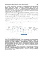
Fig. 52. First Harmonic Centre Paramaters.




Fig. 53. First Harmonic spread parameters.




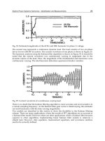
Fig. 54. Mauserd waveform and estimated central of the first harmonic.

Power Quality Harmonics Analysis and Real Measurements Data

62


Fig. 55. 1 st Harmonic with its fuzzy variations.
Figure (87) shows v(t) together with maximum and minimum possible variation (fuzzy) v(t)
can take. It can be observed that the measured v(t) is within the estimated fuzziness and that
the extreme fuzzy variations is shaped up according to the measured v(t).

Fig. 56. Mauserd waveform and ist maximum and minimum fuzzy variation
7.5.5 Two harmonics identification
Next, consider identifying four harmonics at 50Hz, 100Hz, 150 Hz and 200Hz.The voltage
waveform is given in Eq.(102).

( ) 1.414sin(100 0.16667 )
1.0sin(200 0.26667 )
0.3sin(300 0.2 )
0.1sin(400 0.35 )
vt t
t
t
t








(102)

Electric Power Systems Harmonics - Identification and Measurements

63

Then, for estimating the first two harmonics and using Eq.(71) v
1
(k) and v
2
(k) are obtained as
follows:

( ) 1.414sin(0.08 0.16667 )
1
1.0sin(0.16 0.26667 )
() 0.3sin(0.24 0.2 )
2
0.1sin(0.32 0.35 )
vk k
k
vk k
k









(103)
And the linear fuzzy model is given by:
v(k) = A
o

+ A
11
x
11
(k) + A
12
x
12
(k) + A
21
x
21
(k) + A
22
x
22
(k)
Where x
11
(k)=sin(0.08

k), x
12
(k)=cos(0.08

k), x
21
(k)=sin(0.16

k), x

22
(k)=cos(0.16

k).
Therefore, there are nine parameters to be estimated and their estimated values are found to
be:
A
o
= (0.058, 0.0)
A
11
= (1.224, 0.330)
A
12
= (0.707, 0.219)
A
21
= (0.669, 0.267)
A
22
= (0.743, 0.307)
Computing the amplitude and phase:
V
1
= (1.414, 0.395)

1
= (0.166, 0.014)
V
2

= (1.00, 0.406)

2
= (0.266, 0.005)
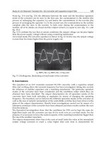
Figures (57-59) show the crisp and fuzzy variations of v(t).







Fig. 57. Efect of removing 2nd Harmonic

Power Quality Harmonics Analysis and Real Measurements Data

64

Fig. 58. Second Harmonic with its fuzzy variation


Fig. 59. Measurd waveform with its fuzzy variations
7.5.6 Conclusion and remarks
In this paper, the harmonics of a non-sinusoidal waveform is identified. The approach is
based on fuzzy Kalman filtering. The basic idea is to identify fuzzy parameters rather than
crisp parameters. The waveform is written as a linear model with fuzzy parameters from
which the amplitude and phase of the harmonics are measured. Kalman filter is used to
identify the fuzzy parameters. Each fuzzy parameter belongs to a triangular symmetric
membership function consisting of center and spread values. Obtaining fuzzy parameters
rather than crisp ones yields all possible extreme variations the parameters can take. This is

useful in designing filters to filter out undesired harmonics that cause distortion.
8. References
J. Arrillaga, D.A. Bradley and P.S. Bodger, “Power System Harmonics,” John Wiley & Sons,
New York, 1985.
IEEE Working Group on Power System Harmonics, “Power System Harmonics: An
Overview,” IEEE Trans. on Power Apparatus and Systems, Vol. PAS-102, No. 8, pp.
2455-2460, August 1983.

Electric Power Systems Harmonics - Identification and Measurements

65
S.A. Soliman, G.S. Christensen, D.H. Kelly and K.M. El-Naggar, “A State Estimation
Algorithm for Identification and Measurement of Power System Harmonics,”
Electrical Power System Research Jr., Vol. 19, pp. 195-206, 1990.
M.S. Saddev and M. Nagpal, “A Recursive Least Error Squares Algorithm for Power System
Relaying and Measurement Applications,” IEEE Trans. on Power Delivery, Vol. 6,
No. 3, pp. 1008-1015, 1991.
S.A. Soliman, K. El-Naggar and A. Al-Kandari, “Kalman Filtering Algorithm for Low
Frequency Power Systems Sub-harmonics Identification,” Int. Jr. of Power and
Energy Systems, Vol. 17, No. 1, pp. 38-43, 1998.
E.A. Abu Al-Feilat, I. El-Amin and M. Bettayeb, “Power System Harmonic Estimation: A
Comparative Study,” Electric Power Systems Research, Vol. 29, pp. 91-97, 1991.
A.A. Girgis, W.B. Chang and E.B. Markram, “A Digital Recursive Measurement Scheme for
On-Line Tracking of Power System Harmonics,” IEEE Trans. on Power Delivery,
Vol. 6, No. 3, pp. 1153-1160, 1991.
H.M. Beides and G.T. Heydt, “Dynamic State Estimation of Power System Harmonics Using
Kalman Filter Methodology,” IEEE Trans. on Power Delivery, Vol. 6, No. 4, pp.
1663-1670, 1991.
H. Ma and A.A. Girgis, “Identification and Tracking of Harmonic Sources in a Power
System Using a Kalman Filter,” IEEE Trans. on Power Delivery, Vol. 11, No. 3, pp.

1659-1665, 1998.
V.M.M. Saiz and J. Barros Gaudalupe, “Application of Kalman Filtering for Continuous
Real-Time Traching of Power System Harmonics,” IEE Proc Gener. Transm.
Distrib. Vol. 14, No. 1, pp. 13-20, 1998.
S.A. Soliman and M.E. El-Hawary, “New Dynamic Filter Based on Least Absolute Value
Algorithm for On-Line Tracking of Power System Harmonics,” IEE Proc
Generation, Trans. Distribution., Vol. 142, No. 1, pp. 37-44, 1005.
S.A. Soliman, K. El-Naggar, and A. Al-Kandari, “Kalman Filtering Based Algorithm for Low
Frequency Power Systems Sub-harmonics Identification,” Int. Jr. of Power and
Energy Systems, Vol. 17, No. 1, pp. 38-43, 1998.
A. Al-Kandari, S.A. Soliman and K. El-Naggar, “Digital Dynamic Identification of Power
System Sub-harmonics Based on Least Absolute Value,” Electric Power Systems
Research, Vol. 28, pp. 99-104, 1993.
A. A. Girgis and J. Qiu, Measurement of the parameters of slowly time varying high
frequency transients, IEEE Trans. On Inst. And Meas., 38(6) (1989) 1057-1062.
A. A. Girgis, M. C. Clapp, E. B. Makram, J. Qiu, J. G. Dalton and R. C. Satoe, Measurement
and characterization of harmonic and high frequency distortion for a large
industrial load, IEEE Trans. Power Delivery, 5(1) (1990) 427-434
A. A. Girgis, W. Chang, and E. B. Makram, Analysis of high-impedance fault generated
signals using a Kalaman filtering approach, IEE Trans. On Power Delivery, 5(4)
(1990).
S. A. Soliman, K. El-Naggar, and A. Al-Kandari, Kalman filtering based algorithm for low
frequency power systems sub-harmonics identification, International Journal of
Power and Energy Systems 17(1), (1997) 38-42.
S. A. Soliman and M. E. El-Hawary, Application of Kalaman filtering for online estimation
of symmetrical components for power system protection, Electric Power Systems
Research 38 (1997) 113-123.

Power Quality Harmonics Analysis and Real Measurements Data

66
S.A. Soliman, I. Helal, and A. M. Al-Kandari, Fuzzy linear regression for measurement of
harmonic components in a power system, Electric Power System Research 50 (1999)
99-105.
L.A. Zadeh, Fuzzy sets as a basis for theory of possibility, Fussy Sets and Systems, Vol. 1, pp
3-28, 1978.
H. Tanaka, S. Vejima, K. Asai, Linear regression analysis with fussy model, IEEE Trans. On
System, Man, and Cybernetics, Vol. 12, No. 6, pp 903-907, 1982.
Timothy J. Ross, Fuzzy logic with engineering applications, McGraw Hill, 1995.
R. G. Brown, Introduction to random signal analysis and Kalman filtering, New York: John
Wiley and Sons, 1983.
G. F. Franklin, J. D. Powel and M. L. Workman, Digital control of dynamic system, 2
nd

edition, Addison Wesley, 1990.
S. K. Tso and W. L. Chan, “Frequency and Harmonic Evaluation Using Non-Linear Least
Squares Techniques” Jr. of Electrical and Electronic Engineers., Australia , Vol. 14,
No. 2, pp. 124-132, 1994.
M. M. Begovic, P. M. Djuric S. Dunlap and A. G. Phadke, “Frequency Tracking in Power
network in the Presence of Harmonics” IEEE Trans. on Power Delivery, Vol. 8, No.
2, pp. 480-486, 1993.
S. A. Soliman, G. S. Christensen, and K. M. El-Naggar, ”A New Approximate Least
Absolute Value Based on Dynamic Filtering for on-line Power System Frequency
Relaying”, Elect. Machines & Power Systems, Vol. 20, pp. 569-592, 1992.
S. A. Soliman, G. S. Christensen, D. H. Kelly, and K. M. El-Naggar, “Dynamic Tracking of
the Steady State Power System Magnitude and Frequency Using Linear Kalman
Filter: a Variable Frequency Model”, Elect. Machines & Power Systems, Vol. 20, pp.
593-611, 1992.
S. A. Soliman and G. S. Christensen, “Estimating of Steady State Voltage and Frequency of
Power Systems from Digitized Bus Voltage Samples”, Elect. Machines & Power

Systems, Vol. 19, pp. 555-576, 1991.
P. K. Dash, D. P. Swain, A. C. Liew, and S. Rahman, “An Adaptive Linear Combiner for on-
line Tracking of Power System Harmonics”, IEEE Trans. on Power Systems,
Vol.114, pp. 1730-1735, 1996.
A. Cavallini and G. C. Montanari, “A Deterministic/Stochastic Framework for Power
System Harmonics Modeling”, IEEE Transaction on Power Systems, Vol.114, 1996.
S. Osowski, “Neural Network for Estimation of Harmonic Components in a Power System”,
IEE Proceeding-C, Vol.139, No.2, pp.129-135, 1992.
S. Osowski, “SVD Technique for Estimation of Harmonic Components in a Power System: a
Statistical Approach”, IEE Proceedings, Gen. Trans. & Distrb., Vol. 141, No.5,
pp.473-479, 1994.
S. A. Soliman , G. S. Christensen, D.H. Kelly, and K. M. El-Naggar, “ Least Absolute Value
Based on Linear Programming Algorithm for Measurement of Power System
Frequency from a Distorted Bus Voltage Signal”, Elect. Machines & Power Systems,
Vol. 20, No. 6, pp. 549-568, 1992.
P. J. Moore, R. D. Carranza and A. T. Johns, “ Model System Tests on a New Numeric
Method of Power System Frequency Measurement” IEEE Transactions on Power
Delivery, Vol. 11, No. 2, pp.696-701, 1996.

Electric Power Systems Harmonics - Identification and Measurements

67
P. J. Moore, J. H. Allmeling and A. T. Johns, “ Frequency Relaying Based on Instantaneous
Frequency Measurement”, IEEE Transaction on Power Delivery, Vol. 11, No. 4,
pp.1737-1742, 1996
T. Lobos and J. Rezmer, “Real -Time Determination of Power System Frequency”, IEEE
Transaction on Instrumentation and Measurement, Vol. 46, No. 4, pp.877-881, 1998.
T. S. Sidhu, and M.S. Sachdev, “An Iterative Techniques for Fast and Accurate Measurement
of Power System Frequency”, IEEE Transaction on Power Delivery, Vol. 13, No. 1,
pp.109-115, 1998.

J. Szafran, and W.,”Power System Frequency Estimation”, IEE Proc Genre. Trans., Distrib.,
Vol. 145, No. 5, pp.578-582, 1998.
T. S. Sidhu, “ Accurate Measurement of Power System Frequency Using a Digital Signal
Processing Technique”, IEEE Transaction on Instrumentation and Measurement,
Vol. 48, No. 1 , pp.75-81, 1999.
P. K. Dash, A. K. Pradhan, and G. Panda, “ Frequency Estimation of Distorted Power System
Signals Using Extended Complex Kalman Filter”, IEEE Transaction on Power
Delivery, Vol. 14, No. 3, pp.761- 766,1999.
S.A. Soliman, H. K Temraz and M. E. El-Hawary, “Estimation of Power System Voltage and
Frequency Using the Three-Phase Voltage Measurements andTransformation”,
Proceeding of Middle East Power System Conference, MEPCON`2000, Cairo, Ain
Shams University, March 2000.
M. E. El-Hawary, “Electric Power Applications of Fuzzy Systems”, IEEE Press, Piscataway,
NJ, 1998.
Quanming Zhang, Huijin Liu, Hongkun Chen, Qionglin Li, and Zhenhuan Zhang,” A
Precise and Adaptive Algorithm for Interharmonics Measurement Based on
Iterative DFT”, IEEE TRANSACTIONS ON POWER DELIVERY, VOL. 23, NO. 4,
OCTOBER 2008.
Walid A. Omran, Hamdy S. K. El-Goharey, Mehrdad Kazerani, and M. M. A. Salama,”
Identification and Measurement of Harmonic Pollution for Radial and Nonradial
Systems”, IEEE TRANSACTIONS ON POWER DELIVERY, VOL. 24, NO. 3, JULY
2009
Ekrem Gursoy, and Dagmar Niebur,” Harmonic Load Identification Using Complex
Independent Component Analysis “,IEEE TRANSACTIONS ON POWER
DELIVERY, VOL. 24, NO. 1, JANUARY 2009
Jing Yong, Liang Chen, and Shuangyan Chen,” Modeling of Home Appliances for Power
Distribution System Harmonic Analysis”, IEEE TRANSACTIONS ON POWER
DELIVERY, VOL. 25, NO. 4, OCTOBER 2010
Elcio F. de Arruda, Nelson Kagan, and Paulo F. Ribeiro,” Harmonic Distortion State
Estimation Using an Evolutionary Strategy”, IEEE TRANSACTIONS ON POWER

DELIVERY, VOL. 25, NO. 2, APRIL 2010
Mohsen Mojiri, Masoud Karimi-Ghartemani and Alireza Bakhshai,” Processing of
Harmonics and Interharmonics Using an Adaptive Notch Filter”, IEEE
TRANSACTIONS ON POWER DELIVERY, VOL. 25, NO. 2, APRIL 2010
Cong-Hui Huang, Chia-Hung Lin, and Chao-Lin Kuo,’ Chaos Synchronization-Based
Detector for Power-Quality Disturbances Classification in a Power System” IEEE
TRANSACTIONS ON POWER DELIVERY, VOL. 26, NO. 2, APRIL 2011

Power Quality Harmonics Analysis and Real Measurements Data

68
Gary W. Chang, Shin-Kuan Chen, Huai-Jhe Su, and Ping-Kuei Wang,” Accurate
Assessment of Harmonic and Interharmonic Currents Generated by VSI-Fed Drives
Under Unbalanced Supply Voltages” IEEE TRANSACTIONS ON POWER
DELIVERY, VOL. 26, NO. 2, APRIL 2011
Abner Ramirez,” The Modified Harmonic Domain: Inter-harmonics” IEEE
TRANSACTIONS ON POWER DELIVERY, VOL. 26, NO. 1, JANUARY 2011
Hooman E. Mazin, Wilsun Xu, and Biao Huang,” Determining the Harmonic Impacts of
Multiple Harmonic-Producing Loads” IEEE TRANSACTIONS ON POWER
DELIVERY, VOL. 26, NO. 2, APRIL 2011.