WIMAX, New Developments 2011 Part 2 pptx

WIMAX,NewDevelopments20

the better the penetration of buildings or of foliage, besides immunity to rainfall, but there is
less bandwidth available.


Fig. 2. Wireless technologies taxonomy (Carcelle et al., 2006)

If we look from the line of sight perspective, wireless technologies can be broadly
categorized into those requiring Line-of-Sight (LOS) and those that do not (NLOS) (Corning,
2005): Line of sight means that there is an unobstructed path from the CPE antenna to the
access point antenna. If the signal can only go from the CPE to the access point by being
reflected by objects, such as trees, the situation is called non-line of sight. NLOS systems are
based on OFDM, which combats multipath interference, thereby permitting the distance
between the CPE and the access point to reach up to 50 kilometers in the MMDS band.
However, NLOS systems are more expensive than LOS systems (Ibe, 2002).

2. WiMAX

WiMAX (Worldwide Interoperability for Microwave Access) is a standardized form of
wireless metropolitan area network (WMAN) technology that has historically been based on
proprietary solutions, such as MMDS and LMDS. The first version of the IEEE 802.16
standard was completed in October 2001 and defines the air interface and medium access
control (MAC) protocol for a wireless metropolitan area network, intended to provide high-
bandwidth wireless voice and data for residential and enterprise use (Ghosh et al., 2005).
This standard was followed by the 802.16a standard in early 2003. Both standards support
peak data rates up to 75 Mbps and have a maximum range of about 50 km. Because WiMAX
systems have the capability to address broad geographic areas without the costly
infrastructure requirement to display cable links to individual sites, the technology may
prove less expensive to expand and should lead to more ubiquitous broadband access (Peng
& Wang, 2007).

Wireless broadband promises to bring high-speed data to multitudes of people in various
geographical locations where wired transmission is too costly, inconvenient, or unavailable

(Salvekar et al., 2004). The 802.16 standard uses Orthogonal Frequency Division Multiple
Access (OFDMA), which is similar to OFDM in the way that it divides the carriers into
multiple sub-carriers. OFDMA, however, goes a step further by then grouping multiple sub-
carriers into sub-channels. A single client or subscriber station might thus transmit using all
of the sub-channels within the carrier space, or multiple clients might also transmit with
each using a portion of the total number of sub-channels simultaneously (Konhauser, 2006).
In the RF front-end, WiMAX uses OFDM, which is robust in adverse channel conditions and
enables NLOS operation. This feature simplifies installation issues and improves coverage,
while maintaining a high level of spectral efficiency. Modulation and coding can be adapted
per burst, ever striving to achieve a balance between robustness and efficiency in accordance
with prevailing link conditions.
Service providers will operate WiMAX both on licensed and unlicensed frequencies. The
technology enables long distance wireless connections with speeds up to 75 Mbps. This can
provide very high data rates and extended coverage. However:
 75 Mbps capacity for the base station is achievable with a 20 MHz channel at best
propagation conditions. But regulators will often allow only smaller channels (10
MHz or less) reducing the maximum bandwidth.
 Even though 50 km is achievable under optimal conditions and with a reduced data
rate (a few Mbps), the typical coverage will be around 5 km with indoor CPE
(NLOS) and around 15 km with a CPE connected to an external antenna (LOS).
 To keep from serving too many customers and thereby greatly reducing each user’s
bandwidth, providers will want to serve no more than 500 subscribers per 802.16
base station (Vaughan-Nichols, 2004).
One of the main advantages of this technology is the capacity to deploy broadband services
in large areas without physical cables. These characteristics give to telecommunication
supplier the capacity to implement new broadband telecommunication infrastructures very
quickly, and with a lower cost than the wired networks.

To sum up, the main advantages of the WiMAX technology in relation to other connection
technologies are: it does not need cable installation, which can solve the access problem to
remote places; it is rather quick to deploy. This technology could have an access velocity
which is 30 times higher than basic ADSL technology. Besides frequency range is between 2
and 11 GHz, with the maximum range of 50 km from the base station, and data transmission
to 70 Mbps. So, one BS sector can serve different businesses or many homes with DSL-rate
connectivity. Another advantage is the high capacity to service modulation (data and voice),
to perform symmetric transmission (the same velocity to send and receive data) and the use
of QoS.

2.1 System Architecture
A fixed broadband wireless access network is essentially a sectorized network, composed of
two key elements: base station (BS) and customer premises equipment (CPE). The BS connects
to the network backbone and uses an outdoor antenna to send and receive high-speed data
and voice to subscriber equipment, thereby eliminating the need for extensive and expensive
wireline infrastructure and providing highly flexible and cost-effective last-mile solutions.
FWA base station equipment multiplexes the traffic from multiple sectors and provides an
interface to the backbone network. For each sector, a radio transceiver module and a sector
antenna is also required. The multiplexer (such as a switch) aggregates the traffic from the
TheRoleofWiMAXTechnologyonBroadbandAccessNetworks:EconomicModel 21

the better the penetration of buildings or of foliage, besides immunity to rainfall, but there is
less bandwidth available.


Fig. 2. Wireless technologies taxonomy (Carcelle et al., 2006)

If we look from the line of sight perspective, wireless technologies can be broadly
categorized into those requiring Line-of-Sight (LOS) and those that do not (NLOS) (Corning,
2005): Line of sight means that there is an unobstructed path from the CPE antenna to the

access point antenna. If the signal can only go from the CPE to the access point by being
reflected by objects, such as trees, the situation is called non-line of sight. NLOS systems are
based on OFDM, which combats multipath interference, thereby permitting the distance
between the CPE and the access point to reach up to 50 kilometers in the MMDS band.
However, NLOS systems are more expensive than LOS systems (Ibe, 2002).

2. WiMAX

WiMAX (Worldwide Interoperability for Microwave Access) is a standardized form of
wireless metropolitan area network (WMAN) technology that has historically been based on
proprietary solutions, such as MMDS and LMDS. The first version of the IEEE 802.16
standard was completed in October 2001 and defines the air interface and medium access
control (MAC) protocol for a wireless metropolitan area network, intended to provide high-
bandwidth wireless voice and data for residential and enterprise use (Ghosh et al., 2005).
This standard was followed by the 802.16a standard in early 2003. Both standards support
peak data rates up to 75 Mbps and have a maximum range of about 50 km. Because WiMAX
systems have the capability to address broad geographic areas without the costly
infrastructure requirement to display cable links to individual sites, the technology may
prove less expensive to expand and should lead to more ubiquitous broadband access (Peng
& Wang, 2007).
Wireless broadband promises to bring high-speed data to multitudes of people in various
geographical locations where wired transmission is too costly, inconvenient, or unavailable

(Salvekar et al., 2004). The 802.16 standard uses Orthogonal Frequency Division Multiple
Access (OFDMA), which is similar to OFDM in the way that it divides the carriers into
multiple sub-carriers. OFDMA, however, goes a step further by then grouping multiple sub-
carriers into sub-channels. A single client or subscriber station might thus transmit using all
of the sub-channels within the carrier space, or multiple clients might also transmit with
each using a portion of the total number of sub-channels simultaneously (Konhauser, 2006).
In the RF front-end, WiMAX uses OFDM, which is robust in adverse channel conditions and

enables NLOS operation. This feature simplifies installation issues and improves coverage,
while maintaining a high level of spectral efficiency. Modulation and coding can be adapted
per burst, ever striving to achieve a balance between robustness and efficiency in accordance
with prevailing link conditions.
Service providers will operate WiMAX both on licensed and unlicensed frequencies. The
technology enables long distance wireless connections with speeds up to 75 Mbps. This can
provide very high data rates and extended coverage. However:
 75 Mbps capacity for the base station is achievable with a 20 MHz channel at best
propagation conditions. But regulators will often allow only smaller channels (10
MHz or less) reducing the maximum bandwidth.
 Even though 50 km is achievable under optimal conditions and with a reduced data
rate (a few Mbps), the typical coverage will be around 5 km with indoor CPE
(NLOS) and around 15 km with a CPE connected to an external antenna (LOS).
 To keep from serving too many customers and thereby greatly reducing each user’s
bandwidth, providers will want to serve no more than 500 subscribers per 802.16
base station (Vaughan-Nichols, 2004).
One of the main advantages of this technology is the capacity to deploy broadband services
in large areas without physical cables. These characteristics give to telecommunication
supplier the capacity to implement new broadband telecommunication infrastructures very
quickly, and with a lower cost than the wired networks.
To sum up, the main advantages of the WiMAX technology in relation to other connection
technologies are: it does not need cable installation, which can solve the access problem to
remote places; it is rather quick to deploy. This technology could have an access velocity
which is 30 times higher than basic ADSL technology. Besides frequency range is between 2
and 11 GHz, with the maximum range of 50 km from the base station, and data transmission
to 70 Mbps. So, one BS sector can serve different businesses or many homes with DSL-rate
connectivity. Another advantage is the high capacity to service modulation (data and voice),
to perform symmetric transmission (the same velocity to send and receive data) and the use
of QoS.

2.1 System Architecture
A fixed broadband wireless access network is essentially a sectorized network, composed of
two key elements: base station (BS) and customer premises equipment (CPE). The BS connects
to the network backbone and uses an outdoor antenna to send and receive high-speed data
and voice to subscriber equipment, thereby eliminating the need for extensive and expensive
wireline infrastructure and providing highly flexible and cost-effective last-mile solutions.
FWA base station equipment multiplexes the traffic from multiple sectors and provides an
interface to the backbone network. For each sector, a radio transceiver module and a sector
antenna is also required. The multiplexer (such as a switch) aggregates the traffic from the
WIMAX,NewDevelopments22

different sectors and forwards it to a router that is connected to the service provider’s
backbone IP network (Ibe, 2002). The backbone connection can be provided with a point-to-
point radio link or a fiber cable, and can be either IP or ATM-based. The distance between
the CPE and the BS depends on how the system is designed and the frequency band in
which it operates. The CPE with an indoor antenna can be installed by the customers
themselves, whereas the outdoor antenna requires a technician to install it (Smura, 2004).
When we need to define a point-to-multipoint wireless system, several parameters are very
important: the characteristics of the geographical area (for example, mountains), the
subscriber density, the bandwidth required, QoS, the number of cells, etc. In areas with a
low traffic demand and/or low subscriber density, the most important factor is the radio
coverage whereas in areas with a high traffic demand and/or high subscriber density,
capacity becomes a more important issue. Through a careful selection of network design
parameters, tradeoffs can be made between coverage and capacity objectives to best serve
the end users within the service area (Wanichkorm, 2002).


Fig. 3. WiMAX System Architecture

The WiMAX wireless link operates with a central BS through a sectorized antenna that is

capable of handling multiple independent sectors simultaneously.

2.2 System Components

As previously referred to, base station equipment and customer premise equipment are the
two main components of WiMAX architecture for the access network. The CPE enables a
user in the customer’s network to access Wide Area Network (WAN). The BS controls the
CPEs within a coverage area, and consists of many access points or wireless hubs, each of
which control the CPE in one sector. The following figure shows the basic components of a
radio communication system.


Fig. 4. Components of a radio communication system (Ibe, 2002)

2.2.1 Customer Premise Equipment – CPE
Residential CPEs are expected to be available in a fully integrated indoor self-installable unit
as well as indoor/outdoor configuration with a high-gain antenna for use on customer sites
with lower signal strength (Ohrtman, 2005). In most cases, a simple plug and play terminal,
similar to a DSL modem, provides connectivity. For customers located several kilometers
away from the WiMAX base station, an outdoor antenna may be required to improve
transmission quality. To serve isolated customers, a directive antenna pointing to the
WiMAX base station may be required.


Fig. 5. FWA Subscriber Configuration (Outdoor CPE)

CPE or terminals are expected to be available in a number of configurations for customer specific
applications and for different types of customers. Households in multi-tenant buildings can be
served by installing a high throughput WiMAX outdoor unit with a low to medium capacity
DSLAM (Digital Subscriber Line Access Multiplexer) as an in-building access device utilizing the

in-building telephone wiring to reach individual apartments or by installing an individual
WiMAX terminal in each household (WiMAX Forum, 2005a). These units are priced higher for
the business case, consistent with the added performance (WiMAX Forum, 2004).
FWA CPE is often divided into three main components parts (Fig. 5): the modem, the radio,
and the antenna. The modem device provides an interface between the customer’s network
and the fixed broadband wireless access network, while the radio provides an interface
TheRoleofWiMAXTechnologyonBroadbandAccessNetworks:EconomicModel 23

different sectors and forwards it to a router that is connected to the service provider’s
backbone IP network (Ibe, 2002). The backbone connection can be provided with a point-to-
point radio link or a fiber cable, and can be either IP or ATM-based. The distance between
the CPE and the BS depends on how the system is designed and the frequency band in
which it operates. The CPE with an indoor antenna can be installed by the customers
themselves, whereas the outdoor antenna requires a technician to install it (Smura, 2004).
When we need to define a point-to-multipoint wireless system, several parameters are very
important: the characteristics of the geographical area (for example, mountains), the
subscriber density, the bandwidth required, QoS, the number of cells, etc. In areas with a
low traffic demand and/or low subscriber density, the most important factor is the radio
coverage whereas in areas with a high traffic demand and/or high subscriber density,
capacity becomes a more important issue. Through a careful selection of network design
parameters, tradeoffs can be made between coverage and capacity objectives to best serve
the end users within the service area (Wanichkorm, 2002).


Fig. 3. WiMAX System Architecture

The WiMAX wireless link operates with a central BS through a sectorized antenna that is
capable of handling multiple independent sectors simultaneously.

2.2 System Components

As previously referred to, base station equipment and customer premise equipment are the
two main components of WiMAX architecture for the access network. The CPE enables a
user in the customer’s network to access Wide Area Network (WAN). The BS controls the
CPEs within a coverage area, and consists of many access points or wireless hubs, each of
which control the CPE in one sector. The following figure shows the basic components of a
radio communication system.


Fig. 4. Components of a radio communication system (Ibe, 2002)

2.2.1 Customer Premise Equipment – CPE
Residential CPEs are expected to be available in a fully integrated indoor self-installable unit
as well as indoor/outdoor configuration with a high-gain antenna for use on customer sites
with lower signal strength (Ohrtman, 2005). In most cases, a simple plug and play terminal,
similar to a DSL modem, provides connectivity. For customers located several kilometers
away from the WiMAX base station, an outdoor antenna may be required to improve
transmission quality. To serve isolated customers, a directive antenna pointing to the
WiMAX base station may be required.


Fig. 5. FWA Subscriber Configuration (Outdoor CPE)

CPE or terminals are expected to be available in a number of configurations for customer specific
applications and for different types of customers. Households in multi-tenant buildings can be
served by installing a high throughput WiMAX outdoor unit with a low to medium capacity
DSLAM (Digital Subscriber Line Access Multiplexer) as an in-building access device utilizing the
in-building telephone wiring to reach individual apartments or by installing an individual
WiMAX terminal in each household (WiMAX Forum, 2005a). These units are priced higher for
the business case, consistent with the added performance (WiMAX Forum, 2004).

FWA CPE is often divided into three main components parts (Fig. 5): the modem, the radio,
and the antenna. The modem device provides an interface between the customer’s network
and the fixed broadband wireless access network, while the radio provides an interface
WIMAX,NewDevelopments24

between the modem and the antenna. As a matter of fact, some vendors integrate these two
components to form a compact CPE, while others have the three units as standalone systems
(Ibe, 2002). The CPE antenna type depends on the Non-Line-of-Sight capabilities of the
system. In a Line-of-Sight FWA network, the CPE antennas are highly directional and
installed outdoors by a professional technician. In Non-Line-of-Sight systems, the
beamwidth of the CPE antenna is typically larger, and in the case of user-installable CPE’s
the antenna should be omnidirectional (Smura, 2004).

2.2.2 Base Station Equipment

The capacity of a single FWA base station sector depends on the channel bandwidth and the
spectral efficiency of the utilized modulation and coding scheme. WiMAX systems take
advantage of adaptive modulation and coding, meaning that inside one BS sector each CPE may
use the most suitable modulation and coding type irrespective of the others (Smura, 2006).


Fig. 6. Base Station components (Ufongene, 1999)

The base station equipment, like CPE, consists of two main building blocks: The antenna
unit and the modulator/demodulator equipment (see Fig. 6 and Fig. 7). The antenna unit
represents the outdoor part of the base station, and is composed of an antenna, a duplexer, a
radio frequency (RF), a low noise amplifier and a down/up converter. The choice of
antennas has a great impact on the capacity and coverage of fixed wireless systems.

The BS consists of one or more radio transceivers, each of which connects to several CPEs

inside a sectorized area. In the BS one directional sector antenna is required for each sector.

Sector antennas are directional antennas and the beamwidth depends both on the service
area and capacity requirements of the system. A BS with one sector using an
omnidirectional antenna has a quarter of the capacity of a four-sector system (Anderson,
2003). The modem equipment modulates and mixes together each flow over the IF cable
which is connected to the antenna unit.


Fig. 7. Base Station components

As we can see in Fig. 7, each FWA base station consists of a number of sectors. The traffic
capacities of these sectors depend most importantly on the modulation and coding methods,
as well as on the bandwidth of the radio channel in use. The sector capacity is divided
between all the subscribers in the sector’s coverage area (Smura, 2004).

3. Techno-Economic Model

To support the new needs of the access networks (bandwidth and mobility), the proposed
framework (Fig. 8) is divided into two perspectives (static and nomadic) and three layers. In
the static perspective, users are stationary and normally require data, voice, and video
quality services. These subscribers demand great bandwidth. In the nomadic/mobility
perspective, the main preoccupation is mobility, and normally, the required bandwidth is
smaller than the static layer (Pereira & Ferreira, 2009).

Focus of the wireless networks was to support mobility and flexibility while that of the
wired access networks is bandwidth and high QoS. However, with the advancement of
technology wireless networks such as WiMAX also geared to provide wideband and high
QoS services competing with wired access networks recently (Fernando, 2008). The
proposed model divides the area into several access networks (the figure is divided into 9

TheRoleofWiMAXTechnologyonBroadbandAccessNetworks:EconomicModel 25

between the modem and the antenna. As a matter of fact, some vendors integrate these two
components to form a compact CPE, while others have the three units as standalone systems
(Ibe, 2002). The CPE antenna type depends on the Non-Line-of-Sight capabilities of the
system. In a Line-of-Sight FWA network, the CPE antennas are highly directional and
installed outdoors by a professional technician. In Non-Line-of-Sight systems, the
beamwidth of the CPE antenna is typically larger, and in the case of user-installable CPE’s
the antenna should be omnidirectional (Smura, 2004).

2.2.2 Base Station Equipment

The capacity of a single FWA base station sector depends on the channel bandwidth and the
spectral efficiency of the utilized modulation and coding scheme. WiMAX systems take
advantage of adaptive modulation and coding, meaning that inside one BS sector each CPE may
use the most suitable modulation and coding type irrespective of the others (Smura, 2006).


Fig. 6. Base Station components (Ufongene, 1999)

The base station equipment, like CPE, consists of two main building blocks: The antenna
unit and the modulator/demodulator equipment (see Fig. 6 and Fig. 7). The antenna unit
represents the outdoor part of the base station, and is composed of an antenna, a duplexer, a
radio frequency (RF), a low noise amplifier and a down/up converter. The choice of
antennas has a great impact on the capacity and coverage of fixed wireless systems.

The BS consists of one or more radio transceivers, each of which connects to several CPEs
inside a sectorized area. In the BS one directional sector antenna is required for each sector.

Sector antennas are directional antennas and the beamwidth depends both on the service

area and capacity requirements of the system. A BS with one sector using an
omnidirectional antenna has a quarter of the capacity of a four-sector system (Anderson,
2003). The modem equipment modulates and mixes together each flow over the IF cable
which is connected to the antenna unit.


Fig. 7. Base Station components

As we can see in Fig. 7, each FWA base station consists of a number of sectors. The traffic
capacities of these sectors depend most importantly on the modulation and coding methods,
as well as on the bandwidth of the radio channel in use. The sector capacity is divided
between all the subscribers in the sector’s coverage area (Smura, 2004).

3. Techno-Economic Model

To support the new needs of the access networks (bandwidth and mobility), the proposed
framework (Fig. 8) is divided into two perspectives (static and nomadic) and three layers. In
the static perspective, users are stationary and normally require data, voice, and video
quality services. These subscribers demand great bandwidth. In the nomadic/mobility
perspective, the main preoccupation is mobility, and normally, the required bandwidth is
smaller than the static layer (Pereira & Ferreira, 2009).

Focus of the wireless networks was to support mobility and flexibility while that of the
wired access networks is bandwidth and high QoS. However, with the advancement of
technology wireless networks such as WiMAX also geared to provide wideband and high
QoS services competing with wired access networks recently (Fernando, 2008). The
proposed model divides the area into several access networks (the figure is divided into 9
WIMAX,NewDevelopments26

sub-areas, but the model can divide the main area between 1 and 36). The central office is

located in the center of the area, and each sub-area will have one or more Aggregation
Nodes (AGN) depending on the technology in use.


Fig. 8. Cost model framework architecture

As we can see in Fig. 8, the framework is separated into three main layers (Pereira, 2007a):
(Layer A) Firstly, we identify the total households and SMEs (Static analysis) for each sub-
area, as well as the total nomadic users (Mobility analysis). The proposed model initially
separates these two components because they have different characteristics. In layer B, the
best technology is analyzed for each Access Network, the static and nomadic components.
For the static analysis we consider the following technologies: FTTH (PON), DSL, HFC, and
WiMAX PLC. For the nomadic analysis we use the WiMAX technology. The final result of
this layer is the best technological solution to support the different needs (Static and

nomadic). The selection of the best option is based on four output results: NPV, IRR, Cost
per subscriber in year 1, and Cost per subscriber in year n. The next step (Layer C) is to
create a single infrastructure that supports the two components. Bearing this in mind, the
tool analyzes each Access Network which is the best solution (based on NPV, IRR, etc).
Then, for each sub-area we verify if the best solution is: a) the use of wired technologies
(FTTH, DSL, HFC, and PLC) to support the static component and the WiMAX technology
for mobility; or b) the use of WiMAX technology to support the Fixed and Nomadic
component.

3.1 Cost Model Structure
The structure of a network depends on the nature of the services offered and their
requirements including bandwidth, symmetry of communication and expected levels of
demand.

Fig. 9. Techno-economic parameters

As shown in Fig. 9, the techno-economic framework basically consists of the following
building blocks (Montagne et al., 2005): Area definition (geography and existing network
infrastructure situation); Service definitions for each user segment with adoption rates and
tariffs, such as network dimensioning rules and cost trends of relevant network equipment;
cost models for investments (CAPEX) and operation costs (OPEX); Discounted cash flow
model; Output metrics to be calculated.
The model analyzes several technical parameters (distances, bandwidth, equipment
performance, etc.) as well as economic parameters (equipment costs, installation costs,
service pricing, demographic distribution, etc.). The model simulates the evolution of the
TheRoleofWiMAXTechnologyonBroadbandAccessNetworks:EconomicModel 27

sub-areas, but the model can divide the main area between 1 and 36). The central office is
located in the center of the area, and each sub-area will have one or more Aggregation
Nodes (AGN) depending on the technology in use.


Fig. 8. Cost model framework architecture

As we can see in Fig. 8, the framework is separated into three main layers (Pereira, 2007a):
(Layer A) Firstly, we identify the total households and SMEs (Static analysis) for each sub-
area, as well as the total nomadic users (Mobility analysis). The proposed model initially
separates these two components because they have different characteristics. In layer B, the
best technology is analyzed for each Access Network, the static and nomadic components.
For the static analysis we consider the following technologies: FTTH (PON), DSL, HFC, and
WiMAX PLC. For the nomadic analysis we use the WiMAX technology. The final result of
this layer is the best technological solution to support the different needs (Static and

nomadic). The selection of the best option is based on four output results: NPV, IRR, Cost

per subscriber in year 1, and Cost per subscriber in year n. The next step (Layer C) is to
create a single infrastructure that supports the two components. Bearing this in mind, the
tool analyzes each Access Network which is the best solution (based on NPV, IRR, etc).
Then, for each sub-area we verify if the best solution is: a) the use of wired technologies
(FTTH, DSL, HFC, and PLC) to support the static component and the WiMAX technology
for mobility; or b) the use of WiMAX technology to support the Fixed and Nomadic
component.

3.1 Cost Model Structure
The structure of a network depends on the nature of the services offered and their
requirements including bandwidth, symmetry of communication and expected levels of
demand.


Fig. 9. Techno-economic parameters

As shown in Fig. 9, the techno-economic framework basically consists of the following
building blocks (Montagne et al., 2005): Area definition (geography and existing network
infrastructure situation); Service definitions for each user segment with adoption rates and
tariffs, such as network dimensioning rules and cost trends of relevant network equipment;
cost models for investments (CAPEX) and operation costs (OPEX); Discounted cash flow
model; Output metrics to be calculated.
The model analyzes several technical parameters (distances, bandwidth, equipment
performance, etc.) as well as economic parameters (equipment costs, installation costs,
service pricing, demographic distribution, etc.). The model simulates the evolution of the
WIMAX,NewDevelopments28

business from 5 to 25 years. This means that each parameter can have a different value each
year, which can be useful for reflecting factors that evolve over time.

3.1.1 General Model Assumptions
Our model framework defines the network starting from a single central office (or head-
end) node and ending at a subscriber CPE. At the CO, we consider only the devices that
support the connection to the access network (OLT).
Users are usually classified in four main categories: Home (residential customers), SOHO
(Small Offices and Home Offices), SME (Small- to Medium-size Enterprises) and LE (Large
Enterprises). The tool implements a methodology for the techno-economic analysis of access
networks for residential customers and SME.

Network
Component
Component Costs Description
Physical
Plant
component
costs
Housing
The housing cost is the cost of building any structures
required (e.g., remote terminal huts and CO buildings),
and includes the cost of permits, labor, and materials.
Cabling
The cabling cost is the cost of the materials (i.e., the cost
of the necessary fiber optic, twisted pair, or coax
cables).
Trenching
The trenching cost is the cost of the labor required to
install the cabling either in underground ducts (buried
trenching) or on overhead poles (aerial trenching).
Network
Equipment

Equipment needed
between CO and
subscriber house
The electronic switches and/or optical devices (e.g.,
splitters) needed to carry the traffic over the physical
plant.
Subscriber Equipment
The price and other properties of the Access node, as
well as the nature of the CPE unit, depend strongly on
the access technology.
Table 1. General Model Assumptions

Access networks (for Wired technologies) have two separate but related components
(Weldon & Zane, 2003): physical plant and network equipment (see Table 1). The physical
plant includes the locations where equipment is placed and the connections between them.
The physical plant costs depend primarily on the labor and real estate costs associated with
the network service area, rather than on the specific technology to expand.
Access network costs can be grouped into two categories (Baker et al., 2007): the costs of
building the network before services can be offered (homes passed), and the costs of
building connections to new subscribers (homes connected). More specifically, the homes
passed portion of costs consists of exchange/CO fit out, feeder cables and civil works,
cabinet and splitters, and distribution cables and civil works. The deployment cost
calculations assumptions suppose that all construction work required to provide service to
all homes passed takes place during the first year (deployment phase). However, only the
necessary electronic equipments are deployed in the CO as well as the aggregation nodes to
accommodate the initial assumption for the take rate.


3.1.2 Input Parameters
As mentioned beforehand, the definition of the input attributes is fundamental to obtain the

right outputs. The model divides the inputs into two main categories: general and specific
input parameters. General parameters are those that describe the area and service
characteristics and are common to all the technologies. The specific parameters are those
that characterize each solution, in technological terms.
These parameters are divided into three main groups: Equipment Components; Cable
Infrastructure and Housing. The housing cost is the price to build any structures required in
the outside plant (Cabinets, closures, etc.) This plant corresponds to the part between CO
and the subscriber house. With regard to the cable infrastructure, the percentage of new
cable corresponds to the need of the new cable required, and the percentage of new conduit
parameter takes into account both underground and aerial lines. The civil work cost is based
on the above mentioned parameters (for example: % of new conduit (Underground/Aerial),
etc.) and on the Database cost. The cost of the labor also takes into account the cabling either
in underground ducts (buried trenching) or on overhead poles (aerial trenching).
To build a new network or upgrade an existing one, an operator has to choose from a set of
technologies. The cost structure may vary significantly from one technology to the other in
terms of up-front costs, variable cost and maintenance costs. Each technology type has
elements which are dedicated, like modems and shared elements (shared by many users)
such as cabinets, optical network units, base stations and cables.
While some costs like equipment pricing, are easy to compute given the data in the Cost
Database, because they do not depend on network topography, the per subscriber cabling
costs (i.e. trenching and fiber) and equipment housing costs (which depend on distance and
density) do, so they require optimization (Weldon & Zane, 2003).
A number of choices, assumptions, and predictions have to be made before proceeding to
the techno-economic analysis of a broadband access network. These include the selection of
the geographical areas and customer segments to be served, the services to be provided, and
the technology to be used to provide the services (Smura, 2006). As we have seen above, the
definition of the input attributes is fundamental to obtain the right outputs. Then, we define
three main activities: Area Definition (Area parameters), Requested Services (Service
parameters), Commercial Parameters and Type of Access.

3.1.3 Output Results
The financial analysis requires several outputs from the tool. The financial analysis is
basically focused on the following steps: to compute the amount of equipment that needs to
be installed each year for providing the service; to compute the amount of money spent on
operational costs (Operations and Maintenance, Customer Support, Service Provisioning,
Marketing); to compute the yearly income, taking into account that existing customers pay
for 12 months; to compute the net profit obtained each year; and the NPV (Net Present
Value) of the yearly profits. The calculated outputs are presented in Table 2:






TheRoleofWiMAXTechnologyonBroadbandAccessNetworks:EconomicModel 29

business from 5 to 25 years. This means that each parameter can have a different value each
year, which can be useful for reflecting factors that evolve over time.

3.1.1 General Model Assumptions
Our model framework defines the network starting from a single central office (or head-
end) node and ending at a subscriber CPE. At the CO, we consider only the devices that
support the connection to the access network (OLT).
Users are usually classified in four main categories: Home (residential customers), SOHO
(Small Offices and Home Offices), SME (Small- to Medium-size Enterprises) and LE (Large
Enterprises). The tool implements a methodology for the techno-economic analysis of access
networks for residential customers and SME.

Network
Component

Component Costs Description
Physical
Plant
component
costs
Housing
The housing cost is the cost of building any structures
required (e.g., remote terminal huts and CO buildings),
and includes the cost of permits, labor, and materials.
Cabling
The cabling cost is the cost of the materials (i.e., the cost
of the necessary fiber optic, twisted pair, or coax
cables).
Trenching
The trenching cost is the cost of the labor required to
install the cabling either in underground ducts (buried
trenching) or on overhead poles (aerial trenching).
Network
Equipment
Equipment needed
between CO and
subscriber house
The electronic switches and/or optical devices (e.g.,
splitters) needed to carry the traffic over the physical
plant.
Subscriber Equipment
The price and other properties of the Access node, as
well as the nature of the CPE unit, depend strongly on
the access technology.
Table 1. General Model Assumptions

Access networks (for Wired technologies) have two separate but related components
(Weldon & Zane, 2003): physical plant and network equipment (see Table 1). The physical
plant includes the locations where equipment is placed and the connections between them.
The physical plant costs depend primarily on the labor and real estate costs associated with
the network service area, rather than on the specific technology to expand.
Access network costs can be grouped into two categories (Baker et al., 2007): the costs of
building the network before services can be offered (homes passed), and the costs of
building connections to new subscribers (homes connected). More specifically, the homes
passed portion of costs consists of exchange/CO fit out, feeder cables and civil works,
cabinet and splitters, and distribution cables and civil works. The deployment cost
calculations assumptions suppose that all construction work required to provide service to
all homes passed takes place during the first year (deployment phase). However, only the
necessary electronic equipments are deployed in the CO as well as the aggregation nodes to
accommodate the initial assumption for the take rate.


3.1.2 Input Parameters
As mentioned beforehand, the definition of the input attributes is fundamental to obtain the
right outputs. The model divides the inputs into two main categories: general and specific
input parameters. General parameters are those that describe the area and service
characteristics and are common to all the technologies. The specific parameters are those
that characterize each solution, in technological terms.
These parameters are divided into three main groups: Equipment Components; Cable
Infrastructure and Housing. The housing cost is the price to build any structures required in
the outside plant (Cabinets, closures, etc.) This plant corresponds to the part between CO
and the subscriber house. With regard to the cable infrastructure, the percentage of new
cable corresponds to the need of the new cable required, and the percentage of new conduit
parameter takes into account both underground and aerial lines. The civil work cost is based
on the above mentioned parameters (for example: % of new conduit (Underground/Aerial),

etc.) and on the Database cost. The cost of the labor also takes into account the cabling either
in underground ducts (buried trenching) or on overhead poles (aerial trenching).
To build a new network or upgrade an existing one, an operator has to choose from a set of
technologies. The cost structure may vary significantly from one technology to the other in
terms of up-front costs, variable cost and maintenance costs. Each technology type has
elements which are dedicated, like modems and shared elements (shared by many users)
such as cabinets, optical network units, base stations and cables.
While some costs like equipment pricing, are easy to compute given the data in the Cost
Database, because they do not depend on network topography, the per subscriber cabling
costs (i.e. trenching and fiber) and equipment housing costs (which depend on distance and
density) do, so they require optimization (Weldon & Zane, 2003).
A number of choices, assumptions, and predictions have to be made before proceeding to
the techno-economic analysis of a broadband access network. These include the selection of
the geographical areas and customer segments to be served, the services to be provided, and
the technology to be used to provide the services (Smura, 2006). As we have seen above, the
definition of the input attributes is fundamental to obtain the right outputs. Then, we define
three main activities: Area Definition (Area parameters), Requested Services (Service
parameters), Commercial Parameters and Type of Access.

3.1.3 Output Results
The financial analysis requires several outputs from the tool. The financial analysis is
basically focused on the following steps: to compute the amount of equipment that needs to
be installed each year for providing the service; to compute the amount of money spent on
operational costs (Operations and Maintenance, Customer Support, Service Provisioning,
Marketing); to compute the yearly income, taking into account that existing customers pay
for 12 months; to compute the net profit obtained each year; and the NPV (Net Present
Value) of the yearly profits. The calculated outputs are presented in Table 2:

WIMAX,NewDevelopments30

Output Description
Cost per subscriber Average cost divided by all subscribers reachable with the system.
Cost per home passed
Average cost divided by all homes reachable with the system.
The cost per home passed will include both the up front costs of
equipment and installation and the ongoing costs of maintaining and
managing the network.
CAPEX Investments costs
OPEX Operation costs
Installation cost Costs for equipment installation
Total expenses CAPEX + OPEX
Total revenue
The total amount customers will pay for their telecommunications
services.
Life Cycle Cost
Is defined as the sum of global discounted investments and global
discounted running costs. This gives the total costs for constructing and
running the network over the study period.
Profit per year (cash
flow)
The Cash Balance (accumulated discounted Cash Flow) curve generally
goes deeply negative because of high initial investments (Monath et al.,
2003). Once revenues are generated, the cash flow turns positive and the
Cash Balance curve starts to rise.
Ending Cash Balance (or

Cumulated Cash Flow)
The balance in the Cash Account at the end of the reporting period and,
therefore, on the ending balance sheet.
Payback Period
(Months)
First year with positive
Net Present Value (NPV
profit)
The NPV is today's value of the sum of resultant discounted cash flows
(annual investments and running costs), or the volume of money which
can be expected over a given period of time.
Internal Rate of Return
(IRR)
IRR is the discount rate at which the NPV is zero. If the IRR is higher
than the opportunity cost of money (that is, interest of an average long
term investment), the project is viable.
Table 2. Output Results

3.2 Access Network Architecture
Our model studies the access part of the network, starting at the central office and ending at
the subscriber’s CPE (see Fig. 10). The cost model is based on a single central office,
connecting the subscribers through several aggregation nodes.

The goal is to optimize the network in order to minimize the cost for a given performance
criterion. The network is sized for the total number of Homes Passed. Consequently, all
infrastructure costs (trenches, housing, electronics and fiber deployment) are incurred for all
Homes Passed. Despite he costs of the CPE’s, ports in the fiber node are only incurred when
a home subscribes.

Fig. 10. Network architecture (Pereira, 2007a)

The access network architecture used in our model is divided into three main segments (Fig.
11): Inside, Outside, and End User. In the CO the different traffic flows are
multiplexed/demultiplexed for further uplink connection to metropolitan and transport
networks or, when it concerns local traffic, switched or routed back to the access network.
For the CO we consider the following components: OLT ports, OLT chassis and passive
splitters.

The outside segment is divided into three main parts: the feeder, aggregation Nodes and
distribution (for HFC technology the distribution segment is divided into distribution and
drop). Feeder segment comprise the network between the CO and the aggregation nodes.
The model includes not only the cost of equipment (Fiber repeaters), but also the optical
fiber cables, installation, trenches, and housing (street cabinets) costs. The ducts can be
shared by several optical fiber cables. The aggregation nodes are located in access areas
street cabinets. The components of these nodes depend on the technology. In the next
section we will present the elements for the five technologies in study. The distribution
network links the aggregation nodes with CPE. Like feeder networks, in distribution, the
model includes not only the cost of equipment (copper, coax, and LV grid repeaters), but
also the cables, installation, and trenches costs.

TheRoleofWiMAXTechnologyonBroadbandAccessNetworks:EconomicModel 31

Output Description
Cost per subscriber Average cost divided by all subscribers reachable with the system.
Cost per home passed
Average cost divided by all homes reachable with the system.
The cost per home passed will include both the up front costs of
equipment and installation and the ongoing costs of maintaining and

managing the network.
CAPEX Investments costs
OPEX Operation costs
Installation cost Costs for equipment installation
Total expenses CAPEX + OPEX
Total revenue
The total amount customers will pay for their telecommunications
services.
Life Cycle Cost
Is defined as the sum of global discounted investments and global
discounted running costs. This gives the total costs for constructing and
running the network over the study period.
Profit per year (cash
flow)
The Cash Balance (accumulated discounted Cash Flow) curve generally
goes deeply negative because of high initial investments (Monath et al.,
2003). Once revenues are generated, the cash flow turns positive and the
Cash Balance curve starts to rise.
Ending Cash Balance (or
Cumulated Cash Flow)
The balance in the Cash Account at the end of the reporting period and,
therefore, on the ending balance sheet.
Payback Period
(Months)
First year with positive
Net Present Value (NPV
profit)
The NPV is today's value of the sum of resultant discounted cash flows
(annual investments and running costs), or the volume of money which
can be expected over a given period of time.

Internal Rate of Return
(IRR)
IRR is the discount rate at which the NPV is zero. If the IRR is higher
than the opportunity cost of money (that is, interest of an average long
term investment), the project is viable.
Table 2. Output Results

3.2 Access Network Architecture
Our model studies the access part of the network, starting at the central office and ending at
the subscriber’s CPE (see Fig. 10). The cost model is based on a single central office,
connecting the subscribers through several aggregation nodes.

The goal is to optimize the network in order to minimize the cost for a given performance
criterion. The network is sized for the total number of Homes Passed. Consequently, all
infrastructure costs (trenches, housing, electronics and fiber deployment) are incurred for all
Homes Passed. Despite he costs of the CPE’s, ports in the fiber node are only incurred when
a home subscribes.



Fig. 10. Network architecture (Pereira, 2007a)

The access network architecture used in our model is divided into three main segments (Fig.
11): Inside, Outside, and End User. In the CO the different traffic flows are
multiplexed/demultiplexed for further uplink connection to metropolitan and transport
networks or, when it concerns local traffic, switched or routed back to the access network.
For the CO we consider the following components: OLT ports, OLT chassis and passive
splitters.

The outside segment is divided into three main parts: the feeder, aggregation Nodes and

distribution (for HFC technology the distribution segment is divided into distribution and
drop). Feeder segment comprise the network between the CO and the aggregation nodes.
The model includes not only the cost of equipment (Fiber repeaters), but also the optical
fiber cables, installation, trenches, and housing (street cabinets) costs. The ducts can be
shared by several optical fiber cables. The aggregation nodes are located in access areas
street cabinets. The components of these nodes depend on the technology. In the next
section we will present the elements for the five technologies in study. The distribution
network links the aggregation nodes with CPE. Like feeder networks, in distribution, the
model includes not only the cost of equipment (copper, coax, and LV grid repeaters), but
also the cables, installation, and trenches costs.

WIMAX,NewDevelopments32


Fig. 11. Block diagram for Access Technologies (Pereira & Ferreira, 2009)

3.2.1 Access Network Components
Table 3 show the components used in our analysis. The components are divided into five
segments (see Fig. 11). The inside plant and feeder segment components are common to all
solutions. Optimally, there would eventually be 32 fibers reaching the ONTs of 32 homes
(Pereira, 2007b). For example if the primary split is 1x4 and the secondary split is 1x8, then
the network splitting ratio (or split scenario) will be 32. This means that a single feeder
network supports 32 subscribers.

Inside Plant
Outside Plant
End User

Feeder Aggregation Node Distribution

1) OLT ports
2) Chassis
3) Splitter
(Primary
Split)
4) Installation:
Ports, chassis,
and split.
1) Optical
repeater
2) Repeater
installation
3)
Aerial/Buried
trenches/ducts
(Trenching
costs)
4) Fiber Cable
(cable cost)
5) Cable
Installation
1) Splitter (Secondary Split)
2) Splitter Installation
3)Housing: Street Cabinet
1) Optical repeater
2) Repeater installation
3) Aerial/Buried
trenches/ducts
(Trenching costs)
4) Fiber Cable (cable cost)

5) Cable Installation
1) ONU
2) Fiber Modem
2) Installation
FTTH(PON)
1) Node Cabinet equipment: ONU;
DSLAM; Splitter; Line-cards;
Chassis; Racks
2) equipment Installation
3)Housing: Street Cabinet
1) Copper regenerator /
repeater
2) Repeater installation
3) Aerial/Buried trenches
(Trenching costs)
4) Copper Cable (cable
cost)
5) Cable Installation
1) xDSL Modem
2) Splitter
3) Installation
xDSL
1) Fiber Node Cabinet equipment:
O/E converter (ONU); RF
combiner
2) equipment Installation
3)Housing: Street Cabinet
1) RF amplifier
2) Amplifier installation

3) Aerial/Buried trenches
(Trenching costs)
4) Coaxial Cable (cable
cost)
5) Cable Installation
1) Cable
Modem
2) Splitter
2) Installation
HFC
1) Local MV/LV Transformer
Station equipment (TE
equipment): O/E converter;
Coupling unit (injection point)
4)Housing: Street Cabinet
2) Transformer Station equipment

3) equipment Installation
1) Repeater for LV
network
2) Installation
1) PLC Modem
2) Installation
PLC
Table 3. Components used for wired technologies

The aggregation node, distribution and end user segments have different components,
depending on each technology. In this table the components for the four wired technologies
used in the model are presented.
The components for WiMAX technology are presented in the next section (see Table 4).

However, the inside plant and feeder components are the same as the wired technologies.

3.2.2 Access Network Architecture for WiMAX
a) System Architecture
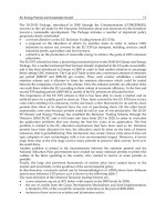
Fig. 12 shows the WiMAX system architecture used in our model. The “air” segments can
replace the distribution and drop segment presented in Table 3.
TheRoleofWiMAXTechnologyonBroadbandAccessNetworks:EconomicModel 33


Fig. 11. Block diagram for Access Technologies (Pereira & Ferreira, 2009)

3.2.1 Access Network Components
Table 3 show the components used in our analysis. The components are divided into five
segments (see Fig. 11). The inside plant and feeder segment components are common to all
solutions. Optimally, there would eventually be 32 fibers reaching the ONTs of 32 homes
(Pereira, 2007b). For example if the primary split is 1x4 and the secondary split is 1x8, then
the network splitting ratio (or split scenario) will be 32. This means that a single feeder
network supports 32 subscribers.

Inside Plant
Outside Plant
End User

Feeder Aggregation Node Distribution

1) OLT ports
2) Chassis
3) Splitter
(Primary
Split)

4) Installation:
Ports, chassis,
and split.
1) Optical
repeater
2) Repeater
installation
3)
Aerial/Buried
trenches/ducts
(Trenching
costs)
4) Fiber Cable
(cable cost)
5) Cable
Installation
1) Splitter (Secondary Split)
2) Splitter Installation
3)Housing: Street Cabinet
1) Optical repeater
2) Repeater installation
3) Aerial/Buried
trenches/ducts
(Trenching costs)
4) Fiber Cable (cable cost)

5) Cable Installation
1) ONU
2) Fiber Modem
2) Installation

FTTH(PON)
1) Node Cabinet equipment: ONU;
DSLAM; Splitter; Line-cards;
Chassis; Racks
2) equipment Installation
3)Housing: Street Cabinet
1) Copper regenerator /
repeater
2) Repeater installation
3) Aerial/Buried trenches
(Trenching costs)
4) Copper Cable (cable
cost)
5) Cable Installation
1) xDSL Modem
2) Splitter
3) Installation
xDSL
1) Fiber Node Cabinet equipment:
O/E converter (ONU); RF
combiner
2) equipment Installation
3)Housing: Street Cabinet
1) RF amplifier
2) Amplifier installation
3) Aerial/Buried trenches
(Trenching costs)
4) Coaxial Cable (cable
cost)
5) Cable Installation

1) Cable
Modem
2) Splitter
2) Installation
HFC
1) Local MV/LV Transformer
Station equipment (TE
equipment): O/E converter;
Coupling unit (injection point)
4)Housing: Street Cabinet
2) Transformer Station equipment
3) equipment Installation
1) Repeater for LV
network
2) Installation
1) PLC Modem
2) Installation
PLC
Table 3. Components used for wired technologies

The aggregation node, distribution and end user segments have different components,
depending on each technology. In this table the components for the four wired technologies
used in the model are presented.
The components for WiMAX technology are presented in the next section (see Table 4).
However, the inside plant and feeder components are the same as the wired technologies.

3.2.2 Access Network Architecture for WiMAX
a) System Architecture
Fig. 12 shows the WiMAX system architecture used in our model. The “air” segments can
replace the distribution and drop segment presented in Table 3.

WIMAX,NewDevelopments34

Base Station
Internet
PSTN
Wireless
Modem
Wireless
Modem
Home
Indoor CPE
Outdoor CPE
Wireless
Modem
Ethernet LAN
Home
Business
WiMAX
Base Station 1
Feeder (Fiber)
Backhaul
Local
Exchange
OLT Port
(Optical Line
Termination)
Fiber Km
O
L
T

Central Office
Cabinet
ONU
Sector 1 Radio
transceiver
Sector N Radio
transceiver
Multiplexer
Base Station
Fiber
Backhaul
Cabinet
ONU
WiMAX
Base Station n
Inside Plant End user
Feeder Segment
Distribution
Segment
Outside Plant
AGN and Base Station
Video
Wireless PMP
Access
Primary Split
(located at CO)

Fig. 12. Block Diagram of the baseline WiMAX system architecture

b) Components

According to the network architecture, the radio access network basically includes base
stations, sites and “last mile” transmission (Wang, 2004). We therefore assume that the
architecture is composed of a BS in the central end, a station in the subscriber side, and a
PMP topology (between BS and CPE).
For capacity limited deployment scenarios it is necessary to position base stations with a BS
to BS spacing sufficient to match the expected density of end customers. Data density is an
excellent metric for matching capacity to market requirements. Demographic information
including population, households and businesses per sq Km is readily available from a
variety of sources for most metropolitan areas. With this information and the expected
services to be offered along with an expected market penetration, data density requirements
are easily calculated (WiMAX Forum, 2005b).
Base stations (towers) and base station equipment does not need to be installed in totality
during the first year, but can be displayed over a period of time to address specific market
segments or geographical areas of interest for the operator. However, in an area with a high
number of potential subscribers, it is desirable to install a sufficient number of base stations
to cover an addressable market large enough to quickly recover the fixed infrastructure cost
(WiMAX Forum, 2004).
As presented in the previous figure, the common cost elements assumed in our model are in
terms of Base Station the upfront costs; sector costs (including transducer and antenna); and
Installation cost (co-siting, new site); Customer Premise Equipment (CPE): Indoor/Outdoor CPE;
and Installation of the CPE, besides Operation, Administration and Maintenance (OAM).

Outside Plant
End User
Aggregation Node (Base Station)
Distribution
(Wireless PMP
Access)
1) Site acquisition
2) Site lease

3) Civil works BS
4) Housing Cabinet / Closures for each BS
5) PMP equipment (multiplexer + cost sector X # sectors
per BS)
6) BS installation Cost (including sectors)
7) ONU (BS) and Installation
air 1) WiMAX
terminal (include:
Antenna,
Transceiver, Radio
Modem)
2) Installation

Table 4. WiMAX architecture components

It is rather important to calculate the required number of FWA base stations and sectors to
fulfill the traffic capacity demands of all the subscribers in a given service area (Smura,
2004). The first step is the prediction of aggregate subscriber traffic in the service area. The
number of the required BS is calculated as a function of the demand specified by the service
area to be covered; average capacity required per user during busy hour; and number of
subscribers within the coverage area (Johansson et al., 2004). When radius of service-area cell
is small, there are many cells of total service area. When the radius of the service-area cell is
large, the number of cells is smaller in a total service area. This is the reason why total
construction relative cost is decreasing when radius of service area is increasing.

3.3 Geometric Model Assumptions
The definition of the geometric model is required to calculate the length of trenches, ducts
and cables. Some of the construction techniques are aerial, using string along utility poles
(mostly rural areas); trench, digging up earth and then lay a new conduit and fiber (used in
urban areas); and pull-through, running through existing underground conduits. Since each

technology has different characteristics, the model assumes different assumptions for the
several access technologies, which are described in the previous sections.

Feeder Networks Distribution Networks
[-2,-1] [-2,1] [-2,2][-2,-2]
[-1,-2] [-1,-1] [-1,1] [-1,2]
[1,-2] [1,-1] [1,1] [1,2]
[2,-1] [2,1] [2,2]
L
L1
Column 1 Column 2Column -2 Column -1
[2,-2]
CO


Table 5. Geometric model for Feeder and Distribution networks

In our work we consider that trench length represents the civil work required for digging
and ducting – the model does not make distinction between aerial (overhead poles) and
TheRoleofWiMAXTechnologyonBroadbandAccessNetworks:EconomicModel 35

Base Station
Internet
PSTN
Wireless
Modem
Wireless
Modem
Home
Indoor CPE

Outdoor CPE
Wireless
Modem
Ethernet LAN
Home
Business
WiMAX
Base Station 1
Feeder (Fiber)
Backhaul
Local
Exchange
OLT Port
(Optical Line
Termination)
Fiber Km
O
L
T
Central Office
Cabinet
ONU
Sector 1 Radio
transceiver
Sector N Radio
transceiver
Multiplexer
Base Station
Fiber
Backhaul

Cabinet
ONU
WiMAX
Base Station n
Inside Plant End user
Feeder Segment
Distribution
Segment
Outside Plant
AGN and Base Station
Video
Wireless PMP
Access
Primary Split
(located at CO)

Fig. 12. Block Diagram of the baseline WiMAX system architecture

b) Components
According to the network architecture, the radio access network basically includes base
stations, sites and “last mile” transmission (Wang, 2004). We therefore assume that the
architecture is composed of a BS in the central end, a station in the subscriber side, and a
PMP topology (between BS and CPE).
For capacity limited deployment scenarios it is necessary to position base stations with a BS
to BS spacing sufficient to match the expected density of end customers. Data density is an
excellent metric for matching capacity to market requirements. Demographic information
including population, households and businesses per sq Km is readily available from a
variety of sources for most metropolitan areas. With this information and the expected
services to be offered along with an expected market penetration, data density requirements
are easily calculated (WiMAX Forum, 2005b).

Base stations (towers) and base station equipment does not need to be installed in totality
during the first year, but can be displayed over a period of time to address specific market
segments or geographical areas of interest for the operator. However, in an area with a high
number of potential subscribers, it is desirable to install a sufficient number of base stations
to cover an addressable market large enough to quickly recover the fixed infrastructure cost
(WiMAX Forum, 2004).
As presented in the previous figure, the common cost elements assumed in our model are in
terms of Base Station the upfront costs; sector costs (including transducer and antenna); and
Installation cost (co-siting, new site); Customer Premise Equipment (CPE): Indoor/Outdoor CPE;
and Installation of the CPE, besides Operation, Administration and Maintenance (OAM).

Outside Plant
End User
Aggregation Node (Base Station)
Distribution
(Wireless PMP
Access)
1) Site acquisition
2) Site lease
3) Civil works BS
4) Housing Cabinet / Closures for each BS
5) PMP equipment (multiplexer + cost sector X # sectors
per BS)
6) BS installation Cost (including sectors)
7) ONU (BS) and Installation
air 1) WiMAX
terminal (include:
Antenna,
Transceiver, Radio
Modem)

2) Installation

Table 4. WiMAX architecture components

It is rather important to calculate the required number of FWA base stations and sectors to
fulfill the traffic capacity demands of all the subscribers in a given service area (Smura,
2004). The first step is the prediction of aggregate subscriber traffic in the service area. The
number of the required BS is calculated as a function of the demand specified by the service
area to be covered; average capacity required per user during busy hour; and number of
subscribers within the coverage area (Johansson et al., 2004). When radius of service-area cell
is small, there are many cells of total service area. When the radius of the service-area cell is
large, the number of cells is smaller in a total service area. This is the reason why total
construction relative cost is decreasing when radius of service area is increasing.

3.3 Geometric Model Assumptions
The definition of the geometric model is required to calculate the length of trenches, ducts
and cables. Some of the construction techniques are aerial, using string along utility poles
(mostly rural areas); trench, digging up earth and then lay a new conduit and fiber (used in
urban areas); and pull-through, running through existing underground conduits. Since each
technology has different characteristics, the model assumes different assumptions for the
several access technologies, which are described in the previous sections.

Feeder Networks Distribution Networks
[-2,-1] [-2,1] [-2,2][-2,-2]
[-1,-2] [-1,-1] [-1,1] [-1,2]
[1,-2] [1,-1] [1,1] [1,2]
[2,-1] [2,1] [2,2]
L
L1
Column 1 Column 2Column -2 Column -1

[2,-2]
CO


Table 5. Geometric model for Feeder and Distribution networks

In our work we consider that trench length represents the civil work required for digging
and ducting – the model does not make distinction between aerial (overhead poles) and
WIMAX,NewDevelopments36

buried (underground ducts). However, the costs are more significant where infrastructure
must be buried than where it can be installed on existing poles (usually, aerial installation is
almost twice as inexpensive as when the infrastructure is buried).

4. Results

4.1 Scenario description


Value
Trend
(% per year)
Years (Study Period) 15
Geographical Area Description
Urban
Total Access Networks (Sub-areas) 4
Area
Characteristics
Area Size (Km2) 47 0,00%
Access Network area (Km2)

11,75
Residential
Total Households (potential subscribers) 11510 1,10%
Households Density (Households / Km2) 245
Population Density (people/Km2) 250 3,80%
Population
11.750
Inhabitants per household 1,02
Technology penetration rate (expected market
penetration)
40,00% 8,00%
Number of subscribers 4.604
Average Households per building 6
Number of buildings in serving area (homes/km2) 1918
SME (small-to-medium sized enterprises)

Total SME in Area 2502 1,50%
Technology penetration rate (expected market
penetration)
30,00% 5,00%
Total SME (customers) 751
Nomadic Users

Total Nomadic Users 1950 15,00%
Service
Characteristics
Residential
Required Downstream bandwidth (Mbps): Avg
data rate
8 1,2%

Required Upstream bandwidth (Mbps): Avg data
rate
0,512 1,2%
SME

Required Downstream bandwidth (Mbps): Avg
data rate
12 1,2%
Required Upstream bandwidth (Mbps): Avg data
rate
0,512 1,2%
Nomadic Users
Required Downstream bandwidth (Mbps): Avg
data rate
2 2,0%
Required Upstream bandwidth (Mbps): Avg data
rate
0,512 2,0%

Pricing
Residential
One-time Activation/connection fee (€) 100 0,15%
Subscription fee (€ / month) 50 0,15%
SME
One-time Activation/connection fee (€) 150 0,15%
Subscription fee (€ / month) 75 0,15%
Nomadic Users
One-time Activation/connection fee (€) 75 0,15%
Subscription fee (€ / month) 45 0,15%
Discount Rate (on cash flows) 0%

Table 6. General Input Parameters for Access Network

The three main activities for the scenario description are: area definition, definition of the set of
services to be offered, and the pricing. Table 6 shows the general input parameters used in our
model and tool.
The trends for each parameter are presented in the last column. This scenario is defined for a
study period of 15 years and for an urban area (City located in a remote area). The definition
of the area type is essential because several costs are influenced by the fact that it is either an
urban or a rural area.
Other important parameter is the definition of the number of access networks in which we
want to divide the studied area (between 1 and 36). This scenario assumes the division of
the area into 4 sub-areas (or access networks). Next, the definition of the number of
households (HH), SMEs and nomadic users is also required for each access network (Table 7).


Access
Network
1
Access
Network
2
Access
Network
3
Access
Network
4
Total
Area
(Year 1)

HH:

9000 2000 500 10
11510
SME:

1000 5000 1000 2
7002
Nomadic Users:

100 850 0 1000
1950
Table 7. Input Parameters: Total subscribers for each Access Network

As mentioned before (see Table 5), the access areas can be divided into five circular areas
(between 1 and 5). This way, we can distribute the users in each access area, and calculate
the trenches and required cable for the wired technologies (Table 8). When using wireless
technologies, this structure is a good option to manage the required base stations for each
access area more effectively.


Access
Network 1
Access
Network 2
Access
Network 3
Access
Network 4

HHs

SMEs

HHs

SMEs

HHs

SMEs

HHs

SMEs
Area1 50% 10% 20%

20% 20% 20% 5% 20%
Area2 20% 20% 20%

20% 20% 20% 10% 20%
Area3 15% 40% 20%

20% 20% 20% 15% 20%
Area4 10% 20% 20%

20% 20% 20% 20% 20%
Area5 5% 10% 20%

20% 20% 20% 50% 20%

Table 8. Input Parameters: Subscribers localization for each Access Network
TheRoleofWiMAXTechnologyonBroadbandAccessNetworks:EconomicModel 37

buried (underground ducts). However, the costs are more significant where infrastructure
must be buried than where it can be installed on existing poles (usually, aerial installation is
almost twice as inexpensive as when the infrastructure is buried).

4. Results

4.1 Scenario description


Value
Trend
(% per year)
Years (Study Period) 15
Geographical Area Description
Urban
Total Access Networks (Sub-areas) 4
Area
Characteristics
Area Size (Km2) 47 0,00%
Access Network area (Km2)
11,75
Residential
Total Households (potential subscribers) 11510 1,10%
Households Density (Households / Km2) 245
Population Density (people/Km2) 250 3,80%
Population
11.750

Inhabitants per household 1,02
Technology penetration rate (expected market
penetration)
40,00% 8,00%
Number of subscribers 4.604
Average Households per building 6
Number of buildings in serving area (homes/km2) 1918
SME (small-to-medium sized enterprises)

Total SME in Area 2502 1,50%
Technology penetration rate (expected market
penetration)
30,00% 5,00%
Total SME (customers) 751
Nomadic Users

Total Nomadic Users 1950 15,00%
Service
Characteristics
Residential
Required Downstream bandwidth (Mbps): Avg
data rate
8 1,2%
Required Upstream bandwidth (Mbps): Avg data
rate
0,512 1,2%
SME

Required Downstream bandwidth (Mbps): Avg
data rate

12 1,2%
Required Upstream bandwidth (Mbps): Avg data
rate
0,512 1,2%
Nomadic Users
Required Downstream bandwidth (Mbps): Avg
data rate
2 2,0%
Required Upstream bandwidth (Mbps): Avg data
rate
0,512 2,0%

Pricing
Residential
One-time Activation/connection fee (€) 100 0,15%
Subscription fee (€ / month) 50 0,15%
SME
One-time Activation/connection fee (€) 150 0,15%
Subscription fee (€ / month) 75 0,15%
Nomadic Users
One-time Activation/connection fee (€) 75 0,15%
Subscription fee (€ / month) 45 0,15%
Discount Rate (on cash flows) 0%
Table 6. General Input Parameters for Access Network

The three main activities for the scenario description are: area definition, definition of the set of
services to be offered, and the pricing. Table 6 shows the general input parameters used in our
model and tool.
The trends for each parameter are presented in the last column. This scenario is defined for a
study period of 15 years and for an urban area (City located in a remote area). The definition

of the area type is essential because several costs are influenced by the fact that it is either an
urban or a rural area.
Other important parameter is the definition of the number of access networks in which we
want to divide the studied area (between 1 and 36). This scenario assumes the division of
the area into 4 sub-areas (or access networks). Next, the definition of the number of
households (HH), SMEs and nomadic users is also required for each access network (Table 7).


Access
Network
1
Access
Network
2
Access
Network
3
Access
Network
4
Total
Area
(Year 1)
HH:

9000 2000 500 10
11510
SME:

1000 5000 1000 2

7002
Nomadic Users: 100 850 0 1000
1950
Table 7. Input Parameters: Total subscribers for each Access Network

As mentioned before (see Table 5), the access areas can be divided into five circular areas
(between 1 and 5). This way, we can distribute the users in each access area, and calculate
the trenches and required cable for the wired technologies (Table 8). When using wireless
technologies, this structure is a good option to manage the required base stations for each
access area more effectively.


Access
Network 1
Access
Network 2
Access
Network 3
Access
Network 4

HHs

SMEs

HHs

SMEs

HHs

SMEs

HHs

SMEs
Area1 50% 10% 20%

20% 20% 20% 5% 20%
Area2 20% 20% 20%

20% 20% 20% 10% 20%
Area3 15% 40% 20%

20% 20% 20% 15% 20%
Area4 10% 20% 20%

20% 20% 20% 20% 20%
Area5 5% 10% 20% 20% 20% 20% 50% 20%
Table 8. Input Parameters: Subscribers localization for each Access Network
WIMAX,NewDevelopments38

4.1.1 Feeder and Distribution Network Parameters
As described in Fig. 11, the feeder segment corresponds to the network part between CO
and the aggregation node. In the CO, our model considers the OLT equipment, and we
assume that the primary splits are at the CO. Table 9 shows the parameters used for the
feeder and distribution segment of the network.

Feeder Network Parameters Distribution Network Parameters
Technology Technology

Primary Split (located at CO) 04 FTTH(PON)
OLT Chassis Secondary Split (Street Cabinet) 08
Number of OLT card slots per OLT
Chassis
16 Split Ratio: Subscribers per OLT port 32
OLT Cards (only for Subs not for HP)
xDSL
Number of OLT ports per Card 08 xDSL technology ADSL
Max. ONU's per OLT Port 64 ONU
Downstream Rate (Mbps) per OLT port 622 Maximum DS Capacity per ONU (Mbps) 2000
Upstream Rate (Mbps) per OLT port 155 Maximum US Capacity per ONU (Mbps) 1000
Optical repeater and Copper regenerator
Remote Terminal DSLAM
Distance between Optical Repeater (km) 30 DSLAM Units (Chassis) 6 Line Cards
Trench Parameters
Number of Line Cards (ATU-Cs) per DSLAM unit:
Slots
6
Total Trench Lenght (Km) 10,28
DSLAM Line Card (only for Subs not for homes
passed)
Line_card_ports_4
8
% of new trenches 65% Number of port per line card (Max. subs per line card) 48
Street Cabinet Parameters Downstream Rate (Mbps) per DSLAM line card port 8,00
% of new Street Cabinets/Closures 60% Upstream Rate (Mbps) per DSLAM line card port 2,00
Max. # of Users per Street
Cabinet(AGN)
2048 user DSLAM Line Card Splitter
Cable Parameters for feeder network DSLAM Splitter Card 48 ports

% of new cable 60% Remote cabinet capacity
Cable type Optical Cable 48Fiber Max. Number of DSLAMs per cabinet 5
Capacity per fiber (Gb/s) 1 Copper regenerator /repeater

Distance Between Copper Repeater (km) 5
HFC
ONU
Maximum DS Capacity per ONU (Mbps) 2000
Maximum US Capacity per ONU (Mbps) 1000
Number of Ports per ONU (for RF modem) 8
RF node modem
Maximum DS Capacity per RF Node Modem (Mbps) 100
Maximum US Capacity per RF Node Modem (Mbps) 100
RF amplifiers (2-way)
Distance Between RF Amplifiers (2-way): km 2
TAP equipment
Number of Drops per TAP 2
WiMAX
ONU
Maximum DS Capacity per ONU (Mbps) 2000
Maximum US Capacity per ONU (Mbps) 1000
Base Station
Downstream Sector capacity (Mbps) 36
Upstream Sector capacity (Mbps) 10
Maximum sector throughput (Mbps): Capacity per
sector
46
Maximum number of sectors per base station 4
Max. Base Station range - radius (km) 3
CPE (only for Subs not for homes passed)

% of Indoor CPE 60%
% of Outdoor CPE 40%
PLC
ONU
Maximum DS Capacity per ONU (Mbps) 2000
Maximum US Capacity per ONU (Mbps) 1000

LV Transformer equipment
Number of MV/LV transformers per Transformer
Substation
1
AVG Number of feeders per MV/LV transformer 8
Downstream LV TE capacity (Mbps):link between TE-
CPEs)
25
Upstream LV TE capacity (Mbps) 25
Max. # HH per MV/LV transformer: (# Subsc per LV
network)
24
PLC Repeater for all LV networks (all homes passed)
AVG Length of the LV lines (m) 0,3
Maximum repeater reach (m) 0,325
Average number of repeaters in Single house 0
Average # repeaters in building (repeater in the meter
room)
1,27
Table 9. Feeder and Distribution Network Parameters

The distribution segment links the aggregation nodes to the customers. The technologies used in
our work are: FTTH(PON), xDSL, HFC, PLC, and WiMAX. As each solution embraces different

characteristics, the previous table shows the parameters used for each one of them.

4.2 Results
This section presents the final results to support the new requirements of broadband access
(fixed and nomadic users). Table 10 shows the results for the use of the several technologies
to support the static layer (HH and SMEs). Each column corresponds to an access network.
The output variables are represented in the lines: Payback period, NPV, IRR, Cost per
subscriber in year 1, and cost per subscriber in year n.


Access
Network 1
Access Network
2
Access
Network 3
Access
Network 4
Total Area


# Fixed Users

10000 2500 1500 12 14012


# Nomadic Users

100 850 0 1000 1950

FTTH
Payback Period 14 21 22 63 33 (Average)
NPV 11.965.382 € - 2.957.765 € - 2.390.925 € - 165.567 € 3.136.297 € (Average)
IRR 3,06% -2,42% -3,43% -13,19% -4,52% (Average)
Cost Subc Y1 10.852 € 16.153 € 18.444 € 48.135 € 25.811 € (Average)
Cost Subc Y15 153 € 189 € 249 € 207 € 203 € (Average)
CAPEX 52.220.733 € 18.694.854 € 11.437.130 € 237.165 € 82.589.882 € (Sum)
OPEX 9.016.542 € 2.407.516 € 1.403.593 € 15.745 € 12.843.396 € (Sum)
WIMAX
Payback Period 14 14 13 55 27 (Average)
NPV 3.821.570 € 978.222 € 890.269 € - 140.025 € 1.523.938 € (Average)
IRR 2,33% 2,33% 3,32% -12,04% -2,13% (Average)
Cost Subc Y1 4.964 € 5.245 € 6.414 € 42.018 € 17.799 € (Average)
Cost Subc Y15 453 € 458 € 484 € 287 € 408 € (Average)
CAPEX 53.374.912 € 13.198.012 € 7.290.309 € 195.945 € 74.059.178 € (Sum)
OPEX 16.006.174 € 3.968.371 € 2.269.220 € 31.423 € 22.275.190 € (Sum)
DSL
Payback Period 20 34 38 61 40 (Average)
NPV - 11.094.161 € - 11.716.167 € - 7.892.363 € - 131.557 € - 6.372.694 € (Average)
IRR -2,21% -7,53% -9,02% -12,74% -7,99% (Average)
Cost Subc Y1 15.968 € 23.909 € 27.281 € 38.812 € 27.354 € (Average)
Cost Subc Y15 173 € 230 € 321 € 260 € 252 € (Average)
CAPEX 74.679.305 € 27.215.883 € 16.787.143 € 204.107 € 118.886.438 € (Sum)
OPEX 9.617.513 € 2.644.889 € 1.555.018 € 14.794 € 13.832.213 € (Sum)
HFC
Payback Period 15 23 26 69 37 (Average)
NPV 4.715.962 € - 5.051.179 € - 3.789.621 € - 180.505 € 248.612 € (Average)
IRR 1,09% -3,82% -5,04% -13,89% -5,95% (Average)
Cost Subc Y1 12.606 € 18.167 € 20.812 € 50.991 € 28.137 € (Average)
Cost Subc Y15 155 € 194 € 264 € 214 € 211 € (Average)

CAPEX 59.287.426 € 20.721.462 € 12.789.876 € 251.477 € 93.050.241 € (Sum)
OPEX 9.199.269 € 2.474.322 € 1.449.543 € 16.371 € 13.139.505 € (Sum)
TheRoleofWiMAXTechnologyonBroadbandAccessNetworks:EconomicModel 39

4.1.1 Feeder and Distribution Network Parameters
As described in Fig. 11, the feeder segment corresponds to the network part between CO
and the aggregation node. In the CO, our model considers the OLT equipment, and we
assume that the primary splits are at the CO. Table 9 shows the parameters used for the
feeder and distribution segment of the network.

Feeder Network Parameters Distribution Network Parameters
Technology Technology
Primary Split (located at CO) 04 FTTH(PON)
OLT Chassis Secondary Split (Street Cabinet) 08
Number of OLT card slots per OLT
Chassis
16 Split Ratio: Subscribers per OLT port 32
OLT Cards (only for Subs not for HP)
xDSL
Number of OLT ports per Card 08 xDSL technology ADSL
Max. ONU's per OLT Port 64 ONU
Downstream Rate (Mbps) per OLT port 622 Maximum DS Capacity per ONU (Mbps) 2000
Upstream Rate (Mbps) per OLT port 155 Maximum US Capacity per ONU (Mbps) 1000
Optical repeater and Copper regenerator
Remote Terminal DSLAM
Distance between Optical Repeater (km) 30 DSLAM Units (Chassis) 6 Line Cards
Trench Parameters
Number of Line Cards (ATU-Cs) per DSLAM unit:
Slots
6

Total Trench Lenght (Km) 10,28
DSLAM Line Card (only for Subs not for homes
passed)
Line_card_ports_4
8
% of new trenches 65% Number of port per line card (Max. subs per line card) 48
Street Cabinet Parameters Downstream Rate (Mbps) per DSLAM line card port 8,00
% of new Street Cabinets/Closures 60% Upstream Rate (Mbps) per DSLAM line card port 2,00
Max. # of Users per Street
Cabinet(AGN)
2048 user DSLAM Line Card Splitter
Cable Parameters for feeder network DSLAM Splitter Card 48 ports
% of new cable 60% Remote cabinet capacity
Cable type Optical Cable 48Fiber Max. Number of DSLAMs per cabinet 5
Capacity per fiber (Gb/s) 1 Copper regenerator /repeater

Distance Between Copper Repeater (km) 5
HFC
ONU
Maximum DS Capacity per ONU (Mbps) 2000
Maximum US Capacity per ONU (Mbps) 1000
Number of Ports per ONU (for RF modem) 8
RF node modem
Maximum DS Capacity per RF Node Modem (Mbps) 100
Maximum US Capacity per RF Node Modem (Mbps) 100
RF amplifiers (2-way)
Distance Between RF Amplifiers (2-way): km 2
TAP equipment
Number of Drops per TAP 2
WiMAX

ONU
Maximum DS Capacity per ONU (Mbps) 2000
Maximum US Capacity per ONU (Mbps) 1000
Base Station
Downstream Sector capacity (Mbps) 36
Upstream Sector capacity (Mbps) 10
Maximum sector throughput (Mbps): Capacity per
sector
46
Maximum number of sectors per base station 4
Max. Base Station range - radius (km) 3
CPE (only for Subs not for homes passed)
% of Indoor CPE 60%
% of Outdoor CPE 40%
PLC
ONU
Maximum DS Capacity per ONU (Mbps) 2000
Maximum US Capacity per ONU (Mbps) 1000

LV Transformer equipment
Number of MV/LV transformers per Transformer
Substation
1
AVG Number of feeders per MV/LV transformer 8
Downstream LV TE capacity (Mbps):link between TE-
CPEs)
25
Upstream LV TE capacity (Mbps) 25
Max. # HH per MV/LV transformer: (# Subsc per LV
network)

24
PLC Repeater for all LV networks (all homes passed)
AVG Length of the LV lines (m) 0,3
Maximum repeater reach (m) 0,325
Average number of repeaters in Single house 0
Average # repeaters in building (repeater in the meter
room)
1,27
Table 9. Feeder and Distribution Network Parameters

The distribution segment links the aggregation nodes to the customers. The technologies used in
our work are: FTTH(PON), xDSL, HFC, PLC, and WiMAX. As each solution embraces different
characteristics, the previous table shows the parameters used for each one of them.

4.2 Results
This section presents the final results to support the new requirements of broadband access
(fixed and nomadic users). Table 10 shows the results for the use of the several technologies
to support the static layer (HH and SMEs). Each column corresponds to an access network.
The output variables are represented in the lines: Payback period, NPV, IRR, Cost per
subscriber in year 1, and cost per subscriber in year n.


Access
Network 1
Access Network
2
Access
Network 3
Access
Network 4

Total Area


# Fixed Users 10000 2500 1500 12 14012


# Nomadic Users 100 850 0 1000 1950

FTTH
Payback Period 14 21 22 63 33 (Average)
NPV 11.965.382 € - 2.957.765 € - 2.390.925 € - 165.567 € 3.136.297 € (Average)
IRR 3,06% -2,42% -3,43% -13,19% -4,52% (Average)
Cost Subc Y1 10.852 € 16.153 € 18.444 € 48.135 € 25.811 € (Average)
Cost Subc Y15 153 € 189 € 249 € 207 € 203 € (Average)
CAPEX 52.220.733 € 18.694.854 € 11.437.130 € 237.165 € 82.589.882 € (Sum)
OPEX 9.016.542 € 2.407.516 € 1.403.593 € 15.745 € 12.843.396 € (Sum)
WIMAX
Payback Period 14 14 13 55 27 (Average)
NPV 3.821.570 € 978.222 € 890.269 € - 140.025 € 1.523.938 € (Average)
IRR 2,33% 2,33% 3,32% -12,04% -2,13% (Average)
Cost Subc Y1 4.964 € 5.245 € 6.414 € 42.018 € 17.799 € (Average)
Cost Subc Y15 453 € 458 € 484 € 287 € 408 € (Average)
CAPEX 53.374.912 € 13.198.012 € 7.290.309 € 195.945 € 74.059.178 € (Sum)
OPEX 16.006.174 € 3.968.371 € 2.269.220 € 31.423 € 22.275.190 € (Sum)
DSL
Payback Period 20 34 38 61 40 (Average)
NPV - 11.094.161 € - 11.716.167 € - 7.892.363 € - 131.557 € - 6.372.694 € (Average)
IRR -2,21% -7,53% -9,02% -12,74% -7,99% (Average)
Cost Subc Y1 15.968 € 23.909 € 27.281 € 38.812 € 27.354 € (Average)
Cost Subc Y15 173 € 230 € 321 € 260 € 252 € (Average)

CAPEX 74.679.305 € 27.215.883 € 16.787.143 € 204.107 € 118.886.438 € (Sum)
OPEX 9.617.513 € 2.644.889 € 1.555.018 € 14.794 € 13.832.213 € (Sum)
HFC
Payback Period 15 23 26 69 37 (Average)
NPV 4.715.962 € - 5.051.179 € - 3.789.621 € - 180.505 € 248.612 € (Average)
IRR 1,09% -3,82% -5,04% -13,89% -5,95% (Average)
Cost Subc Y1 12.606 € 18.167 € 20.812 € 50.991 € 28.137 € (Average)
Cost Subc Y15 155 € 194 € 264 € 214 € 211 € (Average)
CAPEX 59.287.426 € 20.721.462 € 12.789.876 € 251.477 € 93.050.241 € (Sum)
OPEX 9.199.269 € 2.474.322 € 1.449.543 € 16.371 € 13.139.505 € (Sum)
WIMAX,NewDevelopments40

PLC
Payback Period 30 46 51 51 44 (Average)
NPV - 37.581.298 € - 18.359.891 € - 11.979.733 € - 133.062 € - 16.564.697 € (Average)
IRR -6,36% -10,39% -11,81% -12,93% -10,37% (Average)
Cost Subc Y1 21.257 € 29.714 € 34.382 € 38.622 € 31.420 € (Average)
Cost Subc Y15 221 € 267 € 351 € 220 € 264 € (Average)
CAPEX 98.485.189 € 33.056.567 € 20.378.811 € 202.299 € 152.122.866 € (Sum)
OPEX 12.298.765 € 3.447.930 € 2.050.719 € 18.107 € 17.815.521 € (Sum)
Best
Solution
Payback Period FTTH WIMAX WIMAX PLC


NPV FTTH WIMAX WIMAX DSL


IRR FTTH WIMAX WIMAX WIMAX

CostSubsc Y1 WIMAX WIMAX WIMAX PLC


CostSubsc Yn
FTTH FTTH FTTH FTTH


Table 10. Broadband Access General Results

With these results we can identify the best solution for each access network. In general, the
WiMAX technology is the best option for areas with fewer subscribers (area 3 and 4).

4.3 Sensitivity analysis
A sensitivity analysis is a systematic study of how an output result changes as the
assumptions are varied. For the sensitivity analysis we use the tornado diagrams (graphical
sensitivity analysis technique). A tornado diagram provides a graphical display of the
sensitivity of some system responses to uncertainties in the various inputs of that system.
The diagrams show the effects of uncertainties in each input variables on the output of the
analysis. The following table shows the effect of these input variables (first column:
coverage area, potential HH, etc.) on the output variables (Cost per subscriber, payback
period, NPV, IRR, CAPEX, and OPEX).




Cost Per Subscriber PaybackPeriod NPV
Parameters
Names
Low

Parameter
Values
High
Parameter
Values
Variation

(Low
Value)
Variation

(High
Value)
Variation

(Low
Value)
Variation

(High
Value)
Variation
(Low
Value)
Variation
(High
Value)
Coverage Area -50% 50% -0,1% 0,1% 0,0% 0,0% 1,3% -1,3%
Potential HH -55% 55%
4,9% -1,8% 0,0% 7,1% -31,3% 31,0%

Potential SMEs -65% 65% -2,9% 2,5% 7,1% 0,0% -30,2% 29,9%
TakeRate HH -50% 50% 4,0% -1,7% 0,0% 7,1% -28,0% 27,9%
TakeRate SME -55% 55% -2,5% 2,1% 7,1% 0,0% -25,6% 25,5%
Required DS Bandwidth HH -60% 60% -46,4% 46,2% -57,1% 264,3% 1366,1% -1366,1%
Required DS Bandwidth
SME
-55% 55% -7,8% 7,6% -7,1% 28,6% 152,3% -152,3%
Activation Fee HH -50% 50% -0,1% 0,1% 7,1% 0,0% -23,8% 23,8%
Month Fee HH -40% 40% -0,4% 0,4% 264,3% -35,7% -951,4% 951,4%
Activation Fee SME -40% 40%
0,0% 0,0% 0,0% 0,0% -2,2% 2,2%
Month Fee SME -50% 50% -0,1% 0,1% 35,7% -7,1% -163,3% 163,3%
CAPEX: Equipment -50% 50% -21,3% 21,3% -21,4% 64,3% 334,9% -334,9%
CAPEX: Equip. Installation -55% 55% -4,0% 4,0% -7,1% 28,6% 127,9% -127,9%
CAPEX: Housing -50% 50% -20,6% 20,6% -28,6% 257,1% 680,0% -680,0%
CAPEX: Cable -55% 55%
0,0% 0,0% 0,0% 0,0% 0,2% -0,2%
CAPEX: Civil Works -50% 50% -0,5% 0,5% 0,0% 7,1% 14,5% -14,5%
OPEX: Network Operations -55% 55% -0,8% 0,8% -7,1% 35,7% 168,5% -168,5%
OPEX: Equipment -50% 50% -1,5% 1,5% 0,0% 7,1% 22,9% -22,9%
OPEX: Equip. Installation -55% 55% -0,2% 0,2% 0,0% 0,0% 7,7% -7,7%
OPEX: Housing -50% 50%
-1,0% 1,0% 0,0% 7,1% 34,0% -34,0%
OPEX: Civil Works -50% 50% 0,0% 0,0% 0,0% 0,0% 0,4% -0,4%
OPEX: Lease -55% 55% -0,5% 0,5% -7,1% 28,6% 130,8% -130,8%

IRR CAPEX OPEX
Coverage Area -50% 50%
1,4% -1,4% -0,2% 0,2% -0,1% 0,1%
Potential HH -55% 55% 28,3% -10,5% -46,5% 46,3% -46,6% 46,4%
Potential SMEs -65% 65% -22,5% 18,2% -9,7% 9,7% -9,8% 9,8%
TakeRate HH -50% 50% 24,6% -10,0% -42,4% 42,2% -42,4% 42,3%
TakeRate SME -55% 55% -18,9% 15,8% -8,3% 8,1% -8,3% 8,2%
Required DS Bandwidth HH -60% 60%
1687,2% -100,0% -47,0% 46,8% -38,3% 38,2%
Required DS Bandwidth SME -55% 55% 158,6% -151,4% -7,9% 7,7% -6,4% 6,3%
Activation Fee HH -50% 50% -23,6% 23,5% 0,0% 0,0% -1,1% 1,1%
Month Fee HH -40% 40% -100,0% 711,0% 0,0% 0,0% -5,4% 5,4%
Activation Fee SME -40% 40% -2,2% 2,2% 0,0% 0,0% -0,2% 0,2%
Month Fee SME -50% 50%
-167,2% 150,5% 0,0% 0,0% -1,2% 1,2%

CAPEX: Equipment -50% 50% 401,7% -314,5% -23,1% 23,1% 0,0% 0,0%
CAPEX: Equip. Installation -55% 55% 124,6% -128,5% -4,3% 4,3% 0,0% 0,0%
CAPEX: Housing -50% 50% 657,9% -854,0% -22,4% 22,4% 0,0% 0,0%
CAPEX: Cable -55% 55% 0,2% -0,2% 0,0% 0,0% 0,0% 0,0%
CAPEX: Civil Works -50% 50%
14,4% -14,4% -0,6% 0,6% 0,0% 0,0%
OPEX: Network Operations -55% 55% 152,4% -174,0% 0,0% 0,0% -10,3% 10,3%
OPEX: Equipment -50% 50% 23,9% -23,5% 0,0% 0,0% -18,7% 18,7%
OPEX: Equip. Installation -55% 55% 7,6% -7,6% 0,0% 0,0% -3,0% 3,0%
OPEX: Housing -50% 50% 33,3% -33,6% 0,0% 0,0% -13,1% 13,1%
OPEX: Civil Works -50% 50%
0,4% -0,4% 0,0% 0,0% -0,2% 0,2%
OPEX: Lease -55% 55% 118,9% -132,8% 0,0% 0,0% -6,4% 6,4%
Table 11. Sensitivity analysis for WiMAX technology

The tornado diagrams are a series of horizontal bars (one for each variable) around the base
value result. The big bars mean high impact and are on the top of the diagram. The bars
decline in size to the smallest at the bottom, representing the parameter that causes least
change to the base value. The red bars represent the Output for Low Value (negative
variation in parameter), and the blue bars represents the Output for High Value (positive
variation in parameter).


Fig. 13. Sensitivity analysis for WiMAX technology: Cost per subsc. And payback period

As we can see in graph 1 (Fig. 13), the three input variables which influence more the cost
per subscriber are the required downstream bandwidth; equipment costs and housing costs.
The three more critical variables that affect the payback period (graph 2) are bandwidth
0 1000 2000 3000 4000 5000 6000 7000 8000
RequiredDsBandwithHH

CAPEX_Equipment
CAPEX_Housing
RequiredDsBandwithSME
CAPEX_Installation(Equip)
PotentialHH
TakeRateHH
PotentialSMEs
TakeRateSME
OPEX_Equipment
OPEX_Housing
OPEX_Network_Op
CAPEX_Civil_Works
OPEX_Lease
MonthFeeHH
OPEX_Installation(Equip)
CoverageArea
TornadoDiagram‐ CostPerSubscriber/WIMAX
0 10 20 30 40 50 60
RequiredDsBandwithHH
MonthFeeHH
CAPEX_Housing
CAPEX_Equipment
MonthFeeSME
OPEX_Network_Op
RequiredDsBandwithSME
CAPEX_Installation(Equip)
OPEX_Lease
PotentialH H
PotentialSMEs
TakeRateHH

TakeRateSME
ActivationFeeHH
CAPEX_Civil_Works
OPEX_Equipment
OPEX_Housing
TornadoDiagram‐ PaybackPeriod/WIMAX
TheRoleofWiMAXTechnologyonBroadbandAccessNetworks:EconomicModel 41

PLC
Payback Period 30 46 51 51 44 (Average)
NPV - 37.581.298 € - 18.359.891 € - 11.979.733 € - 133.062 € - 16.564.697 € (Average)
IRR -6,36% -10,39% -11,81% -12,93% -10,37% (Average)
Cost Subc Y1 21.257 € 29.714 € 34.382 € 38.622 € 31.420 € (Average)
Cost Subc Y15 221 € 267 € 351 € 220 € 264 € (Average)
CAPEX 98.485.189 € 33.056.567 € 20.378.811 € 202.299 € 152.122.866 € (Sum)
OPEX 12.298.765 € 3.447.930 € 2.050.719 € 18.107 € 17.815.521 € (Sum)
Best
Solution
Payback Period FTTH WIMAX WIMAX PLC


NPV FTTH WIMAX WIMAX DSL


IRR FTTH WIMAX WIMAX WIMAX


CostSubsc Y1 WIMAX WIMAX WIMAX PLC

CostSubsc Yn
FTTH FTTH FTTH FTTH


Table 10. Broadband Access General Results

With these results we can identify the best solution for each access network. In general, the
WiMAX technology is the best option for areas with fewer subscribers (area 3 and 4).

4.3 Sensitivity analysis
A sensitivity analysis is a systematic study of how an output result changes as the
assumptions are varied. For the sensitivity analysis we use the tornado diagrams (graphical
sensitivity analysis technique). A tornado diagram provides a graphical display of the
sensitivity of some system responses to uncertainties in the various inputs of that system.
The diagrams show the effects of uncertainties in each input variables on the output of the
analysis. The following table shows the effect of these input variables (first column:
coverage area, potential HH, etc.) on the output variables (Cost per subscriber, payback
period, NPV, IRR, CAPEX, and OPEX).




Cost Per Subscriber PaybackPeriod NPV
Parameters
Names
Low
Parameter

Values
High

Parameter
Values
Variation

(Low
Value)
Variation

(High
Value)
Variation

(Low
Value)
Variation

(High
Value)
Variation
(Low
Value)
Variation
(High
Value)
Coverage Area -50% 50% -0,1% 0,1% 0,0% 0,0% 1,3% -1,3%
Potential HH -55% 55%
4,9% -1,8% 0,0% 7,1% -31,3% 31,0%
Potential SMEs -65% 65% -2,9% 2,5% 7,1% 0,0% -30,2% 29,9%
TakeRate HH -50% 50% 4,0% -1,7% 0,0% 7,1% -28,0% 27,9%
TakeRate SME -55% 55% -2,5% 2,1% 7,1% 0,0% -25,6% 25,5%

Required DS Bandwidth HH -60% 60% -46,4% 46,2% -57,1% 264,3% 1366,1% -1366,1%
Required DS Bandwidth
SME
-55% 55% -7,8% 7,6% -7,1% 28,6% 152,3% -152,3%
Activation Fee HH -50% 50% -0,1% 0,1% 7,1% 0,0% -23,8% 23,8%
Month Fee HH -40% 40% -0,4% 0,4% 264,3% -35,7% -951,4% 951,4%
Activation Fee SME -40% 40%
0,0% 0,0% 0,0% 0,0% -2,2% 2,2%
Month Fee SME -50% 50% -0,1% 0,1% 35,7% -7,1% -163,3% 163,3%
CAPEX: Equipment -50% 50% -21,3% 21,3% -21,4% 64,3% 334,9% -334,9%
CAPEX: Equip. Installation -55% 55% -4,0% 4,0% -7,1% 28,6% 127,9% -127,9%
CAPEX: Housing -50% 50% -20,6% 20,6% -28,6% 257,1% 680,0% -680,0%
CAPEX: Cable -55% 55%
0,0% 0,0% 0,0% 0,0% 0,2% -0,2%
CAPEX: Civil Works -50% 50% -0,5% 0,5% 0,0% 7,1% 14,5% -14,5%
OPEX: Network Operations -55% 55% -0,8% 0,8% -7,1% 35,7% 168,5% -168,5%
OPEX: Equipment -50% 50% -1,5% 1,5% 0,0% 7,1% 22,9% -22,9%
OPEX: Equip. Installation -55% 55% -0,2% 0,2% 0,0% 0,0% 7,7% -7,7%
OPEX: Housing -50% 50%
-1,0% 1,0% 0,0% 7,1% 34,0% -34,0%
OPEX: Civil Works -50% 50% 0,0% 0,0% 0,0% 0,0% 0,4% -0,4%
OPEX: Lease -55% 55% -0,5% 0,5% -7,1% 28,6% 130,8% -130,8%

IRR CAPEX OPEX
Coverage Area -50% 50%
1,4% -1,4% -0,2% 0,2% -0,1% 0,1%
Potential HH -55% 55% 28,3% -10,5% -46,5% 46,3% -46,6% 46,4%
Potential SMEs -65% 65% -22,5% 18,2% -9,7% 9,7% -9,8% 9,8%
TakeRate HH -50% 50% 24,6% -10,0% -42,4% 42,2% -42,4% 42,3%
TakeRate SME -55% 55% -18,9% 15,8% -8,3% 8,1% -8,3% 8,2%
Required DS Bandwidth HH -60% 60%
1687,2% -100,0% -47,0% 46,8% -38,3% 38,2%
Required DS Bandwidth SME -55% 55% 158,6% -151,4% -7,9% 7,7% -6,4% 6,3%
Activation Fee HH -50% 50% -23,6% 23,5% 0,0% 0,0% -1,1% 1,1%
Month Fee HH -40% 40% -100,0% 711,0% 0,0% 0,0% -5,4% 5,4%
Activation Fee SME -40% 40% -2,2% 2,2% 0,0% 0,0% -0,2% 0,2%
Month Fee SME -50% 50%
-167,2% 150,5% 0,0% 0,0% -1,2% 1,2%
CAPEX: Equipment -50% 50% 401,7% -314,5% -23,1% 23,1% 0,0% 0,0%
CAPEX: Equip. Installation -55% 55% 124,6% -128,5% -4,3% 4,3% 0,0% 0,0%
CAPEX: Housing -50% 50% 657,9% -854,0% -22,4% 22,4% 0,0% 0,0%

CAPEX: Cable -55% 55% 0,2% -0,2% 0,0% 0,0% 0,0% 0,0%
CAPEX: Civil Works -50% 50%
14,4% -14,4% -0,6% 0,6% 0,0% 0,0%
OPEX: Network Operations -55% 55% 152,4% -174,0% 0,0% 0,0% -10,3% 10,3%
OPEX: Equipment -50% 50% 23,9% -23,5% 0,0% 0,0% -18,7% 18,7%
OPEX: Equip. Installation -55% 55% 7,6% -7,6% 0,0% 0,0% -3,0% 3,0%
OPEX: Housing -50% 50% 33,3% -33,6% 0,0% 0,0% -13,1% 13,1%
OPEX: Civil Works -50% 50%
0,4% -0,4% 0,0% 0,0% -0,2% 0,2%
OPEX: Lease -55% 55% 118,9% -132,8% 0,0% 0,0% -6,4% 6,4%
Table 11. Sensitivity analysis for WiMAX technology

The tornado diagrams are a series of horizontal bars (one for each variable) around the base
value result. The big bars mean high impact and are on the top of the diagram. The bars
decline in size to the smallest at the bottom, representing the parameter that causes least
change to the base value. The red bars represent the Output for Low Value (negative
variation in parameter), and the blue bars represents the Output for High Value (positive
variation in parameter).


Fig. 13. Sensitivity analysis for WiMAX technology: Cost per subsc. And payback period

As we can see in graph 1 (Fig. 13), the three input variables which influence more the cost
per subscriber are the required downstream bandwidth; equipment costs and housing costs.
The three more critical variables that affect the payback period (graph 2) are bandwidth
0 1000 2000 3000 4000 5000 6000 7000 8000
RequiredDsBandwithHH
CAPEX_Equipment
CAPEX_Housing
RequiredDsBandwithSME

CAPEX_Installation(Equip)
PotentialHH
TakeRateHH
PotentialSMEs
TakeRateSME
OPEX_Equipment
OPEX_Housing
OPEX_Network_Op
CAPEX_Civil_Works
OPEX_Lease
MonthFeeHH
OPEX_Installation(Equip)
CoverageArea
TornadoDiagram‐ CostPerSubscriber/WIMAX
0 10 20 30 40 50 60
RequiredDsBandwithHH
MonthFeeHH
CAPEX_Housing
CAPEX_Equipment
MonthFeeSME
OPEX_Network_Op
RequiredDsBandwithSME
CAPEX_Installation(Equip)
OPEX_Lease
PotentialH H
PotentialSMEs
TakeRateHH
TakeRateSME
ActivationFeeHH
CAPEX_Civil_Works

OPEX_Equipment
OPEX_Housing
TornadoDiagram‐ PaybackPeriod/WIMAX
WIMAX,NewDevelopments42

(the increase of 60% in bandwidth implies an increase of 264% in payback period),
households month fee (a decrease of 40% in this fee implies an increase of 264%), and
housing costs (an increase of 50% of this feature leads to an increase of 257% in the payback
period).


Fig. 14. Sensitivity analysis for WiMAX technology: NPV and IRR

For NPV and IRR (Fig. 14), the three most critical input variables remain the same as cost
per subscriber and payback period (bandwidth, housing and equipment costs, and month
fee).


Fig. 15. Sensitivity analysis for WiMAX technology: CAPEX and OPEX



‐100000000 ‐50000000 0 50000000 100000000
RequiredDsBandwithHH
MonthFeeHH
CAPEX_Housing
CAPEX_Equipment
OPEX_Network_Op
MonthFeeSME
RequiredDsBandwithSME

OPEX_Lease
CAPEX_Installation(Equip)
OPEX_Housing
PotentialHH
PotentialSMEs
TakeRateHH
TakeRateSME
ActivationFeeHH
OPEX_Equipment
CAPEX_Civil_Works
TornadoDiagram‐ Npv/WIMAX
0 0 0 0 0 0 0 0 0 0 0
RequiredDsBandwithHH
CAPEX_Housing
MonthFeeHH
CAPEX_Equipment
OPEX_Network_Op
MonthFeeSME
RequiredDsBandwithSME
CAPEX_Installation(Equip)
OPEX_Lease
OPEX_Housing
OPEX_Equipment
ActivationFeeHH
PotentialSMEs
PotentialHH
TakeRateSME
TakeRateHH
CAPEX_Civil_Works
TornadoDiagram‐ Irr/WIMAX

0 10000000 20000000 30000000 40000000 50000000 60000000
RequiredDsBandwithHH
PotentialHH
TakeRateHH
CAPEX_Equipment
CAPEX_Housing
PotentialSMEs
TakeRateSME
RequiredDsBandwithSME
CAPEX_Installation(Equip)
CAPEX_Civil_Works
CoverageArea
CAPEX_Cable
TornadoDiagram‐ Capex/WIMAX
0 1000000 2000000 3000000 4000000
PotentialHH
TakeRateHH
RequiredDsBandwithHH
OPEX_Equipment
OPEX_Housing
OPEX_Network_Op
PotentialSMEs
TakeRateSME
OPEX_Lease
RequiredDsBandwithSME
MonthFeeHH
OPEX_Installation(Equip)
MonthFeeSME
ActivationFeeHH
OPEX_Civil_Works

ActivationFeeSME
CoverageArea
OPEX_Cable
TornadoDiagram‐ Opex/WIMAX

5. Conclusion

Nowadays access networks face two main challenges: the increasing bandwidth demand
and mobility trends. All this will require fundamental changes to the operations of access
networks, the functionality of network nodes and the architecture itself. The initial focus of
wireless networks was to support mobility and flexibility, while for the wired access
networks it was both bandwidth and high QoS. However, with the advances in technology,
wireless solutions (such as WiMAX) have the capacity to provide both wideband and high
QoS. WiMAX technology can also offer very high data rates, extended coverage and quickly
deployable alternative to cabled access networks, such as fiber optic links, coaxial systems
using cable modems, and Digital Subscriber Line (DSL) links. At present, WiMAX systems
have the capability to address broad geographic areas without the costly infrastructure
requirement of deploying cable links to individual sites. Besides, the technology may prove
less expensive to disseminate and should lead to more ubiquitous broadband access.
In this context, we present a techno-economic model framework to support the bandwidth
and mobility trends of access networks. The proposed tool performs a detailed comparison
of WiMAX technology with different broadband access technologies (FTTH: PON. xDSL,
HFC and PLC). For that, we identify the critical components of the WiMAX architecture.
The produced results can analyze how the costs vary, calculating the cost per user, cost per
homes passed, payback period, NPV, IRR, end cash balance, CAPEX, OPEX, and so on. For
each sub-area, we describe the best solution, based on the output results.
Finally, we present the results of the sensitivity analysis. This analysis shows the effect of
the input parameters (Coverage Area, Potential HH/SMEs, Take Rate, Required
Downstream Bandwidth, Required Upstream Bandwidth, Activation Fee, Month Fee, etc.)
on the output parameters (Cost per subscriber, Cost per Homes Passed, End cash balance,

Payback period NPV, IRR, CAPEX, and OPEX.) and also identifies the critical parameters
for several technologies. With this information it is possible to define better strategies for
building broadband access networks.

6. References

1. Anderson,H.R. (2003) Fixed Broadband Wireless System Design. John Wiley & Sons.
2. Baker,J., Cagenius,T., Goodwin,C., Hansson,M. & Hatas,M. (2007) Deep-fiber broadband
access networks. ERICSSON REVIEW, 84, 4-8.
3. Carcelle,X., Dang,T. & Devic,C. (2006) Wireless Networks in industrial environments:
State of the art and Issues. In: IFIP Interactive Conference on Ad-Hoc Networking, pp.
141-156. Springer Boston.
4. Corning (2005) Broadband Technology Overview: Optical Fiber. In: Corning.
5. El Zein,G. & Khaleghi,A. (2007) FTTH Explained: Delivering Efficient Customer
Bandwidth and Enhanced Services. In: New Technologies, Mobility and Security,
Labiod,H. & Badra,M. (eds.), pp. 271-179. Springer Netherlands.
6. Fernando,X. (2008) Broadband Access Networks. In: IEEE - International Conference on
Signal Processing, Communications and Networking (ICSCN 08), pp. 380-383. IEEE
International Conference on Signal Processing, Communications and Networking.
7. Fong,G.L. & Nour,K. (2004) Broadband and the Role of Satellite Services. In: pp. 1-19.
TheRoleofWiMAXTechnologyonBroadbandAccessNetworks:EconomicModel 43

(the increase of 60% in bandwidth implies an increase of 264% in payback period),
households month fee (a decrease of 40% in this fee implies an increase of 264%), and
housing costs (an increase of 50% of this feature leads to an increase of 257% in the payback
period).


Fig. 14. Sensitivity analysis for WiMAX technology: NPV and IRR

For NPV and IRR (Fig. 14), the three most critical input variables remain the same as cost
per subscriber and payback period (bandwidth, housing and equipment costs, and month
fee).


Fig. 15. Sensitivity analysis for WiMAX technology: CAPEX and OPEX



‐100000000 ‐50000000 0 50000000 100000000
RequiredDsBandwithHH
MonthFeeHH
CAPEX_Housing
CAPEX_Equipment
OPEX_Network_Op
MonthFeeSME
RequiredDsBandwithSME
OPEX_Lease
CAPEX_Installation(Equip)
OPEX_Housing
PotentialHH
PotentialSMEs
TakeRateHH
TakeRateSME
ActivationFeeHH
OPEX_Equipment
CAPEX_Civil_Works
TornadoDiagram‐ Npv/WIMAX
0 0 0 0 0 0 0 0 0 0 0
RequiredDsBandwithHH

CAPEX_Housing
MonthFeeHH
CAPEX_Equipment
OPEX_Network_Op
MonthFeeSME
RequiredDsBandwithSME
CAPEX_Installation(Equip)
OPEX_Lease
OPEX_Housing
OPEX_Equipment
ActivationFeeHH
PotentialSMEs
PotentialHH
TakeRateSME
TakeRateHH
CAPEX_Civil_Works
TornadoDiagram‐ Irr/WIMAX
0 10000000 20000000 30000000 40000000 50000000 60000000
RequiredDsBandwithHH
PotentialHH
TakeRateHH
CAPEX_Equipment
CAPEX_Housing
PotentialSMEs
TakeRateSME
RequiredDsBandwithSME
CAPEX_Installation(Equip)
CAPEX_Civil_Works
CoverageArea
CAPEX_Cable

TornadoDiagram‐ Capex/WIMAX
0 1000000 2000000 3000000 4000000
PotentialHH
TakeRateHH
RequiredDsBandwithHH
OPEX_Equipment
OPEX_Housing
OPEX_Network_Op
PotentialSMEs
TakeRateSME
OPEX_Lease
RequiredDsBandwithSME
MonthFeeHH
OPEX_Installation(Equip)
MonthFeeSME
ActivationFeeHH
OPEX_Civil_Works
ActivationFeeSME
CoverageArea
OPEX_Cable
TornadoDiagram‐ Opex/WIMAX

5. Conclusion

Nowadays access networks face two main challenges: the increasing bandwidth demand
and mobility trends. All this will require fundamental changes to the operations of access
networks, the functionality of network nodes and the architecture itself. The initial focus of
wireless networks was to support mobility and flexibility, while for the wired access
networks it was both bandwidth and high QoS. However, with the advances in technology,
wireless solutions (such as WiMAX) have the capacity to provide both wideband and high

QoS. WiMAX technology can also offer very high data rates, extended coverage and quickly
deployable alternative to cabled access networks, such as fiber optic links, coaxial systems
using cable modems, and Digital Subscriber Line (DSL) links. At present, WiMAX systems
have the capability to address broad geographic areas without the costly infrastructure
requirement of deploying cable links to individual sites. Besides, the technology may prove
less expensive to disseminate and should lead to more ubiquitous broadband access.
In this context, we present a techno-economic model framework to support the bandwidth
and mobility trends of access networks. The proposed tool performs a detailed comparison
of WiMAX technology with different broadband access technologies (FTTH: PON. xDSL,
HFC and PLC). For that, we identify the critical components of the WiMAX architecture.
The produced results can analyze how the costs vary, calculating the cost per user, cost per
homes passed, payback period, NPV, IRR, end cash balance, CAPEX, OPEX, and so on. For
each sub-area, we describe the best solution, based on the output results.
Finally, we present the results of the sensitivity analysis. This analysis shows the effect of
the input parameters (Coverage Area, Potential HH/SMEs, Take Rate, Required
Downstream Bandwidth, Required Upstream Bandwidth, Activation Fee, Month Fee, etc.)
on the output parameters (Cost per subscriber, Cost per Homes Passed, End cash balance,
Payback period NPV, IRR, CAPEX, and OPEX.) and also identifies the critical parameters
for several technologies. With this information it is possible to define better strategies for
building broadband access networks.

6. References

1. Anderson,H.R. (2003) Fixed Broadband Wireless System Design. John Wiley & Sons.
2. Baker,J., Cagenius,T., Goodwin,C., Hansson,M. & Hatas,M. (2007) Deep-fiber broadband
access networks. ERICSSON REVIEW, 84, 4-8.
3. Carcelle,X., Dang,T. & Devic,C. (2006) Wireless Networks in industrial environments:
State of the art and Issues. In: IFIP Interactive Conference on Ad-Hoc Networking, pp.
141-156. Springer Boston.
4. Corning (2005) Broadband Technology Overview: Optical Fiber. In: Corning.

5. El Zein,G. & Khaleghi,A. (2007) FTTH Explained: Delivering Efficient Customer
Bandwidth and Enhanced Services. In: New Technologies, Mobility and Security,
Labiod,H. & Badra,M. (eds.), pp. 271-179. Springer Netherlands.
6. Fernando,X. (2008) Broadband Access Networks. In: IEEE - International Conference on
Signal Processing, Communications and Networking (ICSCN 08), pp. 380-383. IEEE
International Conference on Signal Processing, Communications and Networking.
7. Fong,G.L. & Nour,K. (2004) Broadband and the Role of Satellite Services. In: pp. 1-19.
WIMAX,NewDevelopments44

8. Galperin,H. (2005) Wireless Networks and Rural Development: Opportunities for Latin
America. Information Technologies and International Development, 2, 47-56.
9. Ghosh,A., Wolter,D.R., Andrews,J.G. & Chen,R. (2005) Broadband wireless access with
WiMax/802.16: current performance benchmarks and future potential.
Communications Magazine, IEEE, 43, 129-136.
10. Ibe,O.C. (2002) Fixed Broadband Wireless Access Networks and Services. John Wiley & Sons,
Inc
11. Ims,L.A., Bhatnagar,A., Østlyngen,E. & Bozorgebrahimi,K. (2004) Towards the next
generation broadband network platform. Telektronikk, 4, 107-125.
12. Johansson,K., FuruskÄar,A. & Karlsson,P. (2004) Relation Between Base Station
Characteristics and Cost Structure in Cellular Systems. In: IEEE PIMRC 2004, IEEE.
13. Konhauser,W. (2006) Broadband wireless access solutions - Progressive challenges and
potential value of next generation mobile networks. Wireless Personal
Communications, 37, 243-259.
14. Lehr,W., Sirbu,M. & Gillett,S. (2004) Municipal Wireless Broadband: Policy and Business
Implications of emerging Access Technologies. In.
15. Lim,C.K., So,P.L., Gunawan,E., Chen,S., Lie,T.T. & Guan,Y.L. (2000) Development of a
test bed for high-speed power line communications. In: pp. 451-456.
16. Little,A.D. (2004) White Paper on Power Line Communications (PLC) - 2004. In: PLC
Utilities Alliance (PUA) (ed.), PLC Utilities Alliance (PUA).
17. Monath,T., Elnegaard,N.K., Cadro,P. & Katsianis,D. (2003) Economics of Fixed Broadband

Access Network Strategies. IEEE Communications Magazine, 163, 132-139.
18. Montagne,R., Causse,A., Elnegaard,N., Ryan,D. & Bråten,L. (2005) Broadband access
roadmap based on market assessment and technical economic analysis. In: pp. 1-
130. Broadwan.
19. Ohrtman,F. (2005) WiMAX Handbook: Building 802.16 Wireless Networks, 1 edn. McGraw-
Hill Professional.
20. Peng,M. & Wang,W. (2007) A Unified Architecture and Key Techniques for Interworking
between WiMAX and Beyond 3G/4G Systems. Wireless Personal Communications,
43, 1-24.
21. Pereira,J.P. (2007a) A Cost Model for Broadband Access Networks: FTTx versus WiMAX.
In: 2007 Second International Conference on Access Networks, pp. 1-8. Second
International Conference on Access Networks.
22. Pereira,J.P. (2007b) Broadband Access Technologies Evaluation Tool (BATET).
Technological and Economic Development of Economy, XIII, 288-294.
23. Pereira,J.P. & Ferreira,P. (2009) Access Networks for Mobility: A Techno-Economic
Model for Broadband Access Technologies. In: TRIDENTCOM 2009 - The 5th
International Conference on Testbeds and Research Infrastructures for the Development of
Networks and Communities, IEEE.
24. Salvekar,A., Sandhu,S., Li,Q., Vuong,M A. & Qian,X. (2004) Multiple-Antenna
Technology in WiMAX Systems. Intel Technology Journal, 8, 229-240.
25. Sarrocco,C. & Ypsilanti,D. (2008) Convergence and Next Generation Networks. In:
OECD (ed.), OECD.
26. Sigurdsson,H.M. (2007) Techno-Economics of Residential Broadband Deployment (PhD
Thesis). In: Technical University of Denmark - Center for Information and
Communication Technologies.

27. Smura,T. (2006) Competitive Potential of WiMAX in the Broadband Access Market: A
Techno-Economic Analysis. Helsinki University of Technology, 1-21.
28. Smura,T. (2004) Techno-Economic Analysis of IEEE 802.16a-Based Fixed Wireless Access
Networks. In: Helsinki University of Technology.

29. Ufongene,C.M. (1999) A model for the cost analysis of wireless access architectures. Bell
Labs Technical Journal, 4, 134-154.
30. Vaughan-Nichols,S.J. (2004) Achieving wireless broadband with WiMax. Computer, 37,
10-13.
31. Wang,J. (2004) Will WiMAX+WLAN Constitute a Substitute to 3G? - A Techno-
Economic Case Study. In: KTH Center for Wireless Systems., Stockholm.
32. Wanichkorm,K. (2002) The role of fixed wireless access networks in the deployment of
broadband service and competition in local telecommunications markets. In:
Carnegie Mellon University.
33. Weldon,M.K. & Zane,F. (2003) The economics of fiber to the home revisited. Bell Labs
Technical Journal, 8, 181-206.
34. WiMAX Forum (2005a) WiMAX: The Business Case for Fixed Wireless Access in
Emerging Markets. In.
35. WiMAX Forum (2005b) WiMAX Deployment Considerations for Fixed Wireless Access
in the 2.5 GHz and 3.5 GHz Licensed Bands. In: WiMAX Forum (ed.).
36. WiMAX Forum (2004) Business Case Models for Fixed Broadband Wireless Access based
on WiMAX Technology and the 802.16 Standard. In: WiMAX Forum (ed.), WiMAX
Forum.