Báo cáo hóa học: " Research Article Practical Quantize-and-Forward Schemes for the Frequency Division Relay Channel" potx

Hindawi Publishing Corporation
EURASIP Journal on Wireless Communications and Networking
Volume 2007, Article ID 20258, 11 pages
doi:10.1155/2007/20258
Research Article
Practical Quantize-and-Forward Schemes for
the Frequency Division Relay Channel
B. Djeumou,
1
S. Lasaulce,
1
and A. G. K lein
2
1
CNRS, Sup
´
el
´
ec, Paris 11, 3 rue Joliot-Curie, 91190 Gif-sur-Yvette, France
2
Worcester Polytechnic Institute, 100 Institute Road, Worcester, MA 01609-2280, USA
Received 6 April 2007; Revised 22 August 2007; Accepted 13 November 2007
Recommended by Mohamed H. Ahmed
We consider relay channels in which the source-destination and relay-destination signals are assumed to be orthogonal and thus
have to be recombined at the destination. Assuming memoryless signals at the destination and relay, we propose a low-complexity
quantize-and-forward (QF) relaying scheme, which exploits the knowledge of the SNRs of the source-relay and relay-destination
channels. Both in static and quasistatic channels, the quantization noise introduced by the relay is shown to be significant in certain
scenarios. We therefore propose a maximum likelihood (ML) combiner at the destination, which is shown to compensate for these
degradations and to provide significant performance gains. The proposed association, which comprises the QF protocol and ML
detector, can be seen, in particular, as a solution for implementing a simple relaying protocol in a digital relay in contrast with the
amplify-and-forward protocol which is an analog solution.

Copyright © 2007 B. Djeumou et al. This is an open access article distributed under the Creative Commons Attribution License,
which permits unrestricted use, distribution, and reproduction in any medium, provided the original work is properly cited.
1. INTRODUCTION
The channels under investigation in this paper are quasistatic
orthogonal relay channels for which orthogonality is defined
accordingly to [1]. Since the source-destination channel is
assumed to be orthogonal to the relay-destination channel
(i.e., the forward channel), the destination receives two dis-
tinct signals. For the channels under consideration, there
are at least two important technical issues: the relaying pro-
tocol and the recombination scheme at the destination. So
far, three main types of relaying protocols have been con-
sidered in the literature: amplify-and-forward (AF), decode-
and-forward (DF), and estimate-and-forward (EF). From
the corresponding works, several observations can be made:
(a) from information-theoretic studies like [1, 2], it appears
that the best choice of the relaying scheme depends on the
source-relay channel (i.e., the backward channel) signal-to-
noise ratio (SNR) and that of the relay-destination channel;
(b) there are not many works dedicated to the design of prac-
tical EF schemes although the EF protocol has the poten-
tial to perform well for a wide range of relay receive SNRs
(in contrast with DF which is generally more suited to rela-
tively high SNRs); (c) the AF protocol is generally chosen for
its simplicity but implementation-related issues are often ig-
nored. In particular, while the DF protocol is clearly suited to
digital implementations, most of the existing research on the
AF protocol makes the questionable assumption that relays
are perfect analog devices which forward a scaled copy of the
received signal.

One of the motivations for the work presented in the pa-
per is precisely to propose low-complexity relaying schemes
(comparable to the AF protocol complexity) that can be im-
plemented in a digital relay transceiver (in contrast with the
AF protocol) and use the knowledge of the SNRs of the for-
ward and backward channels in order for the relay to op-
timally adapt to the forward and backward channel condi-
tions. To achieve these goals, the main solution proposed is
a quantize-and-forward (QF) protocol for which forward-
ing is done on a symbol-by-symbol basis and aims to mini-
mize the mean square error (MSE) between the source signal
and its reconstructed version at the output of the dequan-
tizer at the destination. Some researchers have also referred
to the classic Wyner-Ziv source coding scheme in [3]asQF
[4, 5]. Our practical approach, which ultimately aims to min-
imize the raw bit-error rate (BER) at the destination for a
fixed transmit spectral efficiency and does not exploit error
correcting coding, differs from these information-theoretic
works. It also differs from other practical studies on EF pro-
tocols, such as [6–8] in the sense that the corresponding re-
laying schemes are not analytically optimized by taking the
2 EURASIP Journal on Wireless Communications and Networking
SNRs of the backward and forward channels into account.
Rather, our work is based on the joint source-channel coding
approach originally introduced in [9] for the Gaussian point-
to-point channel where the authors extended the original it-
erative Lloyd algorithm by designing a scalar quantizer that
takes into account the channel through which the quantized
Gaussian source is to be transmitted. The authors of [10]ap-
plied this approach in the context of the binary symmetric

channel (BSC) and proved that the corresponding distortion
is a nonincreasing function of the number of iterations of the
optimization algorithm. In this paper, we further extend the
iterative algorithm of [9] in the context of quasistatic orthog-
onal relay channels by taking into account both the forward
and backward channels and providing a nonrestrictive suf-
ficient condition for convergence of the derived algorithm,
similarly to [10].
This paper is organized as follows: in Section 2, the sig-
nal model for the orthogonal relay channel, main assump-
tions, and notation are given; in Section 3, the proposed QF
scheme and a modified AF scheme are provided; in Section 4,
weproposeanMLdetector(MLD)inordertoaccountfor
the quantization noise introduced by the relay; in Section 5,
the proposed schemes are evaluated in terms of raw BER and
compared with AF, which serves as a reference strategy; con-
cluding remarks are provided in Section 6.
2. SYSTEM MODEL
The source is assumed to be represented by a discrete-time
signal x, which takes its value in the finite set of equiprob-
able symbols X
={x
1
, , x
M
s
} and is subject to a unit av-
erage power constraint: E[
|x
2

|] = 1. For sake of simplicity,
square M
s
-QAM symbols with independent real and imag-
inary parts are assumed. More importantly, the samples of
the source, denoted by x(n)wheren is the time index, are as-
sumed to be independent and identically distributed (i.i.d.)
as in [9, 10]. In the context of digital communications, this
assumption is generally valid because of interleaving, dither-
ing, or equivalent operations. In order to limit the relay and
receiver complexity, we will not exploit the interactions be-
tween the quantizer and the error correcting coders, possi-
bly present at the source and relay. Therefore the assumption
made on the source samples and channel model (described
just below) implies that there is loss of optimality by assum-
ing scalar quantizers, that is, symbol-by-symbol forwarding
at the relay, instead of vector quantizers [11]. At each time
instant n the source broadcasts the signal x(n), which is re-
ceived by the destination and relay nodes. The received base-
band signals can be written:
y
sd
(n) = h
sd
×x(n)+w
sd
(n),
x
sr
(n) = h

sr
×x(n)+w
sr
(n),
(1)
where w
sd
and w
sr
are zero-mean circularly symmetric com-
plex Gaussian noises with variances σ
2
sd
and σ
2
sr
,respectively.
The complex coefficients h
sd
and h
sr
are, respectively, the
gains of the source-destination and source-relay channels. In
this paper, for simplicity of presentation, most of the deriva-
tions are conducted for static channels, so h
sd
and h
sr
are
constant over the whole transmission. Therefore, the pres-

ence of these gains makes only sense in the quasi-static case
whereas in the context of static channels they could be re-
moved. In this case, these quantities are assumed to be con-
stant over a block duration and vary from block to block. In
the simulation part both cases will be analyzed and Rayleigh
block-fading will be assumed for modeling the channel gains
in the case of quasistatic channels. In this case, for each block,
h
sd
and h
sr
are the realizations of two independent Gaussian
complex random variables. Note that, thanks to the indepen-
dency assumption between all the fading gains, the presence
of the relay will provide more degrees of freedom in the chan-
nel, which will be exploited at the receiver through signal
combiners that will provide a diversity order of two instead of
one (this assertion can be proven for the two combiners pro-
vided in this paper, for more information see [12]). There-
fore, one has to keep in mind that in quasistatic channels
the performance gain due to the presence of the relay can
also come from the qualities of the source-relay and relay-
destination channels but is, in general, essentially due to the
higher diversity order. In static channels (namely, Gaussian
channels or fading channels with a strong Rician compo-
nent) only a gain in terms of SNR can be expected.
The relay forwards the cooperation signal x
r
(n) to the
destination. We assume memoryless and zero-delay relaying.

The memoryless assumption is a consequence of the previ-
ously mentioned independence assumptions while the zero-
delay assumption can be satisfied by resynchronizing the di-
rect and cooperation signals at the destination. Under these
assumptions x
r
(n) = f (x
sr
(n)) for some memoryless func-
tion which is chosen to satisfy a unit average power con-
straint E[
|x
r
|
2
] = 1. Since the relay function and channels
are memoryless, in the sequel we will at times omit the time
index n from the signals. For the QF protocol the relaying
function comprises a zero-memory quantization operation
(denoted by Q)followedbyanM
r
-QAM modulation (de-
noted by M). In the case of the clipped AF protocol, there is
no modulation since the relay is assumed to generate a con-
tinuous signal. The cooperation signal received at the desti-
nation is written:
y
rd
(n) = h
rd

×x
r
(n)+w
rd
(n)
= h
rd
× f

h
sr
x(n)+w
sr
(n)

+ w
rd
(n),
(2)
where the notation is defined above. Orthogonality between
the received cooperation signal y
rd
and direct signal y
sd
can
be implemented by frequency division (FD). The optimal
bandwidth allocation issue is beyond the scope of this paper,
thus we assume that y
sd
and y

rd
have the same bandwidth.
At the destination, two types of combiners can be as-
sumed. We will use either a conventional maximum ratio
combiner (MRC) or a more sophisticated detector, namely
the MLD, which will be derived in Section 4.Thereason
for introducing the latter combiner will be clearly explained
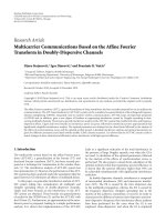
in Section 4. Figure 1 summarizes the system model when
QF is assumed. The notation D stands for decoder, which
jointly incorporates the demodulation and de-quantization
operations. On the other hand, when the relay amplifies-
and-forward, D is the identity operator and Q and M are
B. Djeumou et al. 3
x
h
sr
w
sr
x
sr
h
sd
w
sd
QM
D
x
sr
x
r

y
rd
h
rd
w
rd
x
rd
y
sd
x
Combiner
Figure 1: System model for the quantize-and-forward protocol.
replaced with a linear function in the AF case and a nonlin-
ear function in the clipped AF case (Section 3.2).
3. RELAYING SCHEMES
3.1. Optimum quantize-and-forward
The most natural way to quantize and forward the signal re-
ceived by the relay is to quantize x
sr
in order to minimize the
distortion D
00
 E[|x
sr
− x
sr
|
2
], map the quantizer output

onto a QAM modulation and send it to the destination. As
σ
2
rd
→0 and the number or quantization bits increases, this
quantization strategy becomes optimum since it achieves the
performance of a 1
×2 single-input multiple-output (SIMO)
system. On the other hand, if x
sr
is quantized with a high
number of bits and sent through a bad cooperation channel,
minimizing D
00
is no longer optimal. This is why minimiz-
ing D
01
 E[|x
rd
− x
sr
|
2
]canbemoreefficient as shown by
[9, 10, 13, 14] in the context of the point-to-point Gaussian
channel. In the context of the relay channel we know that the
source-relay channel quality also plays a role in the receiver
performance. Therefore, we propose minimizing the MSE
between the reconstructed signal
x

rd
and the original source
signal x, that is, D
11
 E[|x
rd
−x|
2
], by assuming the SNRs of
the forward and backward channels are known to the relay.
The disadvantage of minimizing D
11
is that in the high co-
operation regime the SIMO performance is not reached. We
will comment on this point further (Section 5.2).
Let us turn our attention to the quantizer itself. Since
the signal to be quantized is complex, the quantizer is com-
posed of two “subquantizers,” one for the real part of x
sr
and
one for its imaginary part. Quantizing consists in mapping
the signal x
sr
into a pair of rational numbers belonging to
V
R
× V
I
={v
R

1
, v
R
2
, , v
R
L
}×{v
I
1
, v
I
2
, , v
I
L
},whereL= 2
b/2
and b is the total number of quantization bits. As the real
and imaginary parts of the signal received by the relay are as-
sumed to be independent, the two subquantizers can be de-
signed independently and in the same manner. This is why,
from now on, we restrict our attention to the subquantizer of
the real part of x
sr
. The subquantizer maps x
R
sr
 Re(x
sr

)onto
the finite set of representatives
{v
R
1
, v
R
2
, , v
R
L
}.LetU
R
=
{
u
R
1
, u
R
2
, , u
R
L+1
}be the set of the transition levels of the sub-
quantizer. The aforementioned mapping is done as follows:
if x
R
sr
∈ S

R
j
= [u
R
j
, u
R
j+1
) then its representative is v
R
j
,where
j
∈{1, 2, ,L}. The quantizer output is then mapped onto
the constellation following the idea of [15]. The mapping is
done in such a manner that close representatives in the signal
space are assigned to close symbols in the modulation space.
Therefore, the most likely decision errors which appear in the
neighborhood of the symbol associated with the input repre-
sentative will result in a slight increase in distortion. We now
describe the quantizer optimization procedure. To find the
optimal pair of subquantizers at the relay, we minimize the
MSE D
11
as follows. The distortion can be written as
D
11
 E





x
rd
−x


2

=
E



x
R
rd

2

−
2E


x
R
rd
x
R


+ E


x
R

2


 
D
R
11
+ E



x
I
rd

2

−
2E


x
I
rd

x
I

+ E


x
I

2


 
D
I
11
.
(3)
As D
R
11
and D
I
11
can be optimized independently and iden-
tically, we focus, hence forth, on minimizing D
R
11
. The latter
quantity can be shown to expand as

D
R
11
=

j

x
R
j

2
p
j
−2

j
x
R
j
p
j
L

=1
v
R

L


k=1
P
R
k,

u
R
k+1
u
R
k
φ

t −x
R
j

dt
+

j
p
j
L

=1

v
R



2
L

k=1
P
R
k,

u
R
k+1
u
R
k
φ

t −x
R
j

dt,
(4)
where
∀j ∈{1, ,

M
s
}, p
j

= Pr[X
R
= x
R
j
] (i.e., the chan-
nel input statistics),
∀(k,) ∈{1, , L}
2
, P
R
k,
= Pr[x
R
rd
=
v
R

|x
R
sr
= v
R
k
] (i.e., the forward channel statistics) and φ(t) =
(|h
sr
|/
√

πσ
sr
)exp(−|h
sr
|
2
t
2
/σ
2
sr
) is the probability density
function (pdf) of the real noise component Re(w
sr
) of the
signal received by the relay (i.e., the backward channel statis-
tics). Given a number of quantization bits, we now opti-
mize the subquantizer Q
R
by minimizing D
R
11
with respect
to the transition levels
{u
R

}
∈{1, ,L}
and the representatives

{v
R

}
∈{1, ,L}
. For fixed transition levels, the optimum repre-
sentatives are the centroids of the corresponding quantiza-
tion cells which are obtained by setting the partial derivatives
of D
R
11
to zero:
v
R

=

√
M
s
k=1
x
R
k
p
k

L
j
=1

P
R
j,

u
R
j+1
u
R
j
φ

t −x
R
k

dt

√
M
s
k=1
p
k

L
j
=1
P
R

j,

u
R
j+1
u
R
j
φ

t −x
R
k

dt
. (5)
When the representatives are fixed, it is not trivial, in gen-
eral, to determine the transition levels explicitly as is the case
for conventional channel optimized quantizers such as [10]
for which the backward channel is not present. The difficulty
is due to the presence of the function φ(
·) in the MSE ex-
pression (for more information see Appendix A). Determin-
ing the transition levels then requires the use of an exhaus-
tive search algorithm. However, note that there are simple
cases such as a 4-QAM source, which is used in the sim-
ulations (Section 5), where both the optimum representa-
tives for fixed transition levels and optimum transition lev-
els for fixed representatives can be found. For a 4-QAM
4 EURASIP Journal on Wireless Communications and Networking

constellation, we have (x
R
, x
I
) ∈{−A,+A}
2
.Forfixedtran-
sition levels, we have for all 
∈{1, , L} that
v
R,∗

= A ×

L
k
=1
P
R
k,

u
R
k+1
u
R
k

φ(t − A) − φ(t + A)


dt

L
k=1
P
R
k,

u
R
k+1
u
R
k

φ(t − A)+φ(t + A)

dt
,(6)
and for fixed representatives we have
u
R,∗

=
σ
2
sr
2A
ln



L
k=1

P
R
,k
−P
R

−1,k

A +(1/2)v
R
k

v
R
k

L
k
=1

P
R
,k
−P
R


−1,k

A − (1/2)v
R
k

v
R
k

.
(7)
Note that in (7) the strict positiveness of the argument of the
logarithm ensures the existence of the optimum transition
levels. We are now in position to provide the complete itera-
tive optimization procedure. Let i and
 be the iteration index
and the current value of the estimation error criterion of the
iterative algorithm. The algorithm is said to have converged
when
 reaches 
max
.
(i) Step 1. Set i = 0. Set  = 1. Initialize V
R
and U
R
with the sets (say V
R
(0)

and U
R
(0)
) obtained from [10],
which correspond to a local optimum since the back-
ward channel is not taken into account.
(ii) Step 2. Set i
→i+1. For the fixed partition U
R
(i
−1)
use (6)
to find the optimal codebook V
R
(i)
. For the fixed code-
book V
R
(i)
use (7) to obtain the optimal partition U
R
(i)
.
If the realizability condition u
R
1
≤ u
R
2
··· ≤u

R
L
is not
met, stop the procedure and keep the transition levels
provided by the previous iteration.
(iii) Step 3. Update
 as follows:
 =

L
k=1


v
R
k(i)
−v
R
k(i
−1)



L
k=1


v
R
k(i)



. (8)
If
 ≥ 
max
, then go to Step 2, stop otherwise.
As with other iterative algorithms (e.g., the EM algo-
rithm), one cannot easily prove or ensure, in general, con-
vergence to the global optimum. When the backward chan-
nel was not present, the authors of [10] proved that the dis-
tortion obtained by applying the generalized Lloyd algorithm
is a nonincreasing function of the number of iterations. The
authors provided a sufficient condition under which the pro-
cedure is guaranteed to converge towards a local optimum.
The corresponding condition is not restrictive since it can be
imposed through the realizability constraint of the transition
levels [10] to the iterative procedure without loss of optimal-
ity. Recall that this constraint consists in imposing u
R

to be
an increasing function of .Itturnsoutasimilarresultcan
be derived in our context (see Appendix A)ifoneassumesa
zero-mean channel input (i.e., E[X
R
] = 0) and the backward
channel noise to be Gaussian. The obtained condition is as
follows: at each iteration step,
∀ ∈{1, , L − 1}, E[


X
R
rd
|

X
R
sr
= v
R
+1
] >E[

X
R
rd
|

X
R
sr
= v
R

]. If this condition is met, the
MSE will be a nonincreasing function of the iteration index.
To conclude this section we will make a few comments
on the complexity of the proposed protocol. Compared to
vector quantizers [16], the proposed solution is much sim-

pler since the creation, storage and computation complexi-
ties (for more information see, e.g., [17]) both grow expo-
nentially with the cell dimension (which is 1 for scalar quan-
tizers). If one wants to further decrease the complexity of the
quantizer, it is possible to simplify the proposed algorithm
by imposing the quantizer to be uniform (equispaced transi-
tion levels and representatives). Since the uniform quantizer
is entirely specified by its quantization step there is only one
parameter to be determined. We will not conduct a complex-
ity analysis here but it can be checked (Appendix C) that the
ratio of the optimum QF protocol complexity to that of the
uniform version is of the order of the number of iterations of
the proposed algorithm, which is typically between 5 and 10
in simulations. The uniform QF protocol can be obtained by
using [9] and by specializing the results presented here. The
performance of the corresponding scheme will be presented
in the simulation part.
3.2. Clipped amplify-and-forward
In this section, we propose a modified version of the AF pro-
tocol. Our motivation for proposing this new version of AF is
threefold. First, it optimizes the same performance criterion
as for the QF schemes, that is, the end-to-end distortion. Sec-
ond, it allows us to fairly compare the scalar QF schemes with
the scalar AF scheme given the fact that the conventional AF
does not exploit the knowledge of the SNRs of the source-
relay and relay-destination channels. Third, the clipped AF
bridges the gap between the QF and AF protocols since it
allows us to isolate the clipping effect naturally introduced
by the QF schemes. So, we now replace the quantizer with a
piecewise linear saturation function, which simply clips sam-

ples with magnitude above a chosen threshold β>0. The lin-
ear threshold function which operates independently on the
real and imaginary parts of the signal is defined as
f
R
β

x
R

=

x
R
,


x
R


≤
β,
β
·sgn

x
R

,



x
R


>β,
(9)
where we considered the case of the real part. We see that
the relay acts like a perfect AF relay in the region [
−β, β]and
limits values outside this region. Our motivation for using
this function is to assess the benefits from clipping x
sr
but in
some context better relaying functions can be used. For ex-
ample the authors of [18] derived the best relaying function
in the sense of the raw BER when no direct link is assumed
and a BPSK modulation is used both at the source and re-
lay. In our context, the goal is different and the extension of
[18] to the case of QAM modulations does not seem to be
trivial. In the same spirit, [19] proposed an optimized relay-
ing function in the sense of the mutual information when no
direct link is assumed. The rationale for the proposed func-
tion (9) is that it preserves the important soft information
but does not needlessly expend power relaying large noise
B. Djeumou et al. 5
samples. Furthermore, it only requires the optimization of
a single parameter, that is, the clipping level β. In spite of the
seeming simplicity of the relaying function, however, calcu-

lating the p.d.f. of saturated Gaussian signals is known to be
intractable [20]. After passing the received signal through the
saturation function, the signal is scaled by some real param-
eter α which is chosen to satisfy the average unit power con-
straint. Of course, in order to ensure coherent reception at
the relay node, the incoming signal also has to be equalized.
Here, our choice is the MMSE (minimum MSE) equalizer:
x
R
sr
(n) = Re[x
sr
(n) ×(h
∗
sr
/|h
sr
|
2
)]. Thus, the cooperation sig-
nal is x
r
(n) = α[ f
R
β
(x
R
sr
(n)) + jf
I

β
(x
I
sr
(n))], where α is such
that E[
|x
r
|
2
] = 1, and f
R
β
(·)and f
I
β
(·)aredefinedidenti-
cally since the real and imaginary parts are assumed to be
i.i.d. Due to the fact that the data and noise are independent
and by calculating the first and the second-order moments
(Appendix B) for the random clipped gaussian variable, we
find that
E


x
r


2

= α
2
E

f
2
β

x
R
sr

+ f
2
β

x
I
sr

=
2α
2
E

f
2
β

x

R
sr

=
2α
2

M
s

x
R

σ
2
sr
2


h
sr


2
+

x
R

2

+

β
2
−
σ
2
sr
2


h
sr


2
−

x
R

2

×

Q

β + x
R
σ

sr
/
√
2


h
sr



+ Q

β −x
R
σ
sr
/
√
2


h
sr



−
σ
sr

2
√
π


h
sr



β + x
R

e
−(β−x
R
)
2
/σ
2
sr
/|h
sr
|
2
+

β−x
R


e
−(β+x
R
)
2
/(σ
2
sr
/|h
sr
|
2
)


(10)
which can be set equal to 1 to find the scaling factor α
β
that
satisfies the power constraint. Note that Q is the classical er-
ror function: Q(x)
= (1/
√
2π)

∞
x
e
−t
2

dt. To find the clip-
ping level β, we minimize the MSE between the source signal
andthe signal received by the destination on the cooperation
channel:
J(β)
= E





1
α
β
h
∗
rd


h
rd


2
y
rd
−x





2

(11)
= E





f
β

x
R
sr

+ j·f
β

x
I
sr

+
1
α
β
h
∗

rd


h
rd


2
w
rd
−x




2

(12)
=
2

M
s

x
R

E

f

2
β

x
R
+
w
R
sr
h
sr

−
2x
R
f
β

x
R
+
w
R
sr
h
sr

+
σ
2

rd
α
2
β


h
rd


2
+1

,
(13)
where we note that α
β
is effectively a function of β since any
change in the clipping level affects the scaling required to sat-
isfy the power constraint. The β that minimizes this func-
tion cannot be written in closed form. However, it is purely
a function of the source-relay and relay-destination SNRs,
so it can be computed numerically offline using (13)and
the calculation of the first and second-order moments for
the clipped Gaussian (Appendix B) and stored in a lookup
table. Note that this implies that the relay needs to know
the SNRs on its channel both to the transmitter as well as
to the receiver, which was also the case in the QF proto-
col.
4. COMBINING SCHEMES

When the AF protocol is assumed at the relay, the optimum
combiner in terms of raw BER is the MRC. When using the
clipped version of the AF protocol this is no longer true since
the equivalent additive noise in the relay-destination chan-
nel is not Gaussian. As already mentioned, calculating the
pdf of saturated Gaussian signals is known to be intractable.
Therefore, we will still use the MRC at the destination when
the clipped AF is used. We will see through the simulation
analysis that this issue does not seem to be critical but de-
riving a better combiner might be seen as an extension of
this work. On the other hand, when QF is assumed, using
the MRC at the destination can lead to a significant perfor-
mance loss. In this respect the authors have shown in [21]
that using the DF protocol with a conventional MRC when
the relay is in bad reception conditions can severely degrade
the BER performance at the destination with respect to the
case without cooperation. This is in part because the relay
generates non-Gaussian residual decoding noise that is cor-
related with the useful signal. For the QF protocol the com-
biner choice might look less critical since the relay does not
make a decision on the transmitted symbols. However, for a
low number of quantization bits and relay receive SNR, the
answer is not clear. This is why we not only consider the MRC
but also propose a more sophisticated detector (namely, the
MLD) adapted to the QF protocol, which is derived as fol-
lows.
Assume the symbol transmitted by the source is x and
the quantizer output Q(x
sr
) = v

i
. The likelihood p
ML
=
p(y
sd
, x
rd
| x) can be factorized as
p
ML
= p

y
sd
| x

p


x
rd
| x, y
sd

=
p

y
sd

| x

p

y
sd
| x
rd
, x

p


x
rd
, x

p

y
sd
| x

p

x

=
p


y
sd
| x

p

y
sd
| x

p


x
rd
| x

p

x

p

y
sd
| x

p

x


=
p

y
sd
| x

p


x
rd
| x

,
(14)
where p(y
sd
| x) = (1/πσ
2
sd
)exp(−|y
sd
−h
sd
x|
2
/σ
2

sd
). To ex-
pand the second term p(
x
rd
| x), we recall that

X
rd
∈ V
R
×
V
I
={v
1
, v
2
, , v
M
r
}, and we make use of the channel tran-
sitions probabilities P
k,
between complex representatives
6 EURASIP Journal on Wireless Communications and Networking
9876543210
SNR
sr
(dB)

10
−4
10
−3
10
−2
10
−1
BER
R
X
without coop
Uniform QF minimizing D
11
with b = 2
Uniform QF minimizing D
11
with b = 6
SIMO bound
Figure 2: Influence of b on the performance when the uniform QF
protocol is used over static channels: raw BER versus SNR
sr
at the
output of the MRC for SNR
rd
= 10 dB with SNR
sr
= SNR
sd
+10dB.

(see Section 3.1) where we have defined P
R
k,
for the real part
of complex representatives. We have
p


x
rd
= v
i
| x

=

x
sr
p

x
sr
, x
rd
= v
i
| x

dx
sr

=

x
sr
p

x
sr
| x

p


x
rd
= v
i
| x
sr

dx
sr
=
M
r

j=1


x

sr
∈S
j
p

x
sr
| x

p

x
rd
= v
i
| x
sr

dx
sr

=
M
r

j=1
P
j,i



x
sr
∈S
j
p

x
sr
| x

dx
sr

=
√
(M
r
)

=1
√
(M
r
)

m=1
P
j,i
×



u
R
+1
u
R

φ

t −x
R

dt

u
I
m+1
u
I
m
φ

t

−x
I

dt



,
(15)
where the index j corresponds the symbol of the relay alpha-
bet (i.e.,
{1, , M
r
}) associated with the pair of representa-
tives (v
R

, v
I
m
). Now, by denoting s = (s
1
, , s
N
), the vector of
bits associated with the source symbol x allows us to express
the log-likelihood ratio for the nth bit:
λ

s
n

=
log
⎡
⎣


s∈S
(n)
1
p

y
sd
| x

p

x
rd
| x


s∈S
(n)
0
p

y
sd
| x

p


x
rd

| x

⎤
⎦
,
(16)
where the sets S
(i)
1
and S
(i)
0
are defined by S
(n)
1
={(s
1
, , s
N
)
∈{0, 1}
N
| s
n
=1}and S
(n)
0
={(s
1
, , s

N
)∈{0, 1}
N
| s
n
= 0}.
If λ(s
n
) > 0, then s
n
= 1ands
n
= 0 otherwise.
5. SIMULATION ANALYSIS
We assume a 4-QAM source and consider different simula-
tion scenarios with the following parameters:
(i) the channels can be either static (Gaussian or purely
Rician) or quasistatic (Rayleigh block-fading model);
in the latter case the channels are constant over a block
duration; each block comprises 100 symbols; we note
that the case of static channels can correspond to real
situations in wireless communications, for example,
fixed users using laptops connected to a hot-spot;
(ii) the relative quality of the relay: SNR
sr
[dB] =
SNR
sd
[dB] + ρ,whereρ ∈{−5dB,0dB,+10dB};
(iii) the number of quantization bits used by the QF proto-

col: b
∈{2, 6} (i.e., b/2 bits per subquantizer);
(iv) the relay-destination channel quality: SNR
rd
[dB] ∈
{
0dB,10dB,30dB} with SNR
rd
= 1/σ
2
rd
;
(v) the relaying scheme: AF, optimally clipped AF, uniform
QF, and optimum QF; for reference, we will consider
the case where no relay is available (a BPSK is then
used at the transmitter in order to make a fair com-
parison in terms of spectral efficiency) and also the full
cooperation case; the latter is defined as follows: σ
rd
→0
and the AF protocol is used; we will refer to this case as
the SIMO bound;
(vi) the combining scheme at the receiver: MRC or MLD.
5.1. Optimum QF versus uniform QF
All the simulations we performed showed one significant
drawback of the uniform QF relaying protocol. Both in static
and quasistatic channels, the receiver performance, when us-
ing the uniform QF protocol with MRC or MLD, is sensitive
to the choice of the number of quantization bits. This ten-
dency is clearly more marked for static channels. For exam-

ple, see Figures 2 and 3. Figure 2 shows that using the uni-
form QF with b
= 6 bits can lead to a significant performance
loss. This appears when the source-relay SNR is sufficiently
large and the cooperation channel has medium quality. In
this situation it is better to decode and forward than quantize
and forward a signal that is not robust to cooperation chan-
nel noise. When b/2
= 1 the uniform QF roughly behaves like
DF while it behaves more like AF for b
= 6, which explains
why the performance is better for b
= 6inFigure 3.Our
interpretation is that the uniform QF has only one degree
of freedom (namely, its quantization step) to adapt to SNR
sr
and SNR
rd
. For a fixed number of bits, there will always be
scenarios where the performance of the uniform QF can be
much less than the optimum relaying scheme (AF, DF, or op-
timum QF) used in the considered setup. On the other hand,
the number of quantization bits has much less influence on
the performance of the optimum QF when the MLD is em-
ployed at the receiver. By analyzing many simulations, which
arenotprovidedhereduetolackofspace,wehaveobserved
B. Djeumou et al. 7
3210−1−2−3−4
SNR
sr

(dB)
10
−4
10
−3
10
−2
10
−1
BER
R
X
without coop
Uniform QF minimizing D
11
with b = 2
Uniform QF minimizing D
11
with b = 6
SIMO bound
Figure 3: Influence of b on the performance when the uniform QF
protocol is used over static channels: raw BER versus SNR
sr
at the
output of the MRC for SNR
rd
= 10 dB with SNR
sr
= SNR
sd

−5dB.
that it is generally better to choose a sufficiently high num-
ber of bits (typically 3 bits per dimension) regardless of the
SNRs of the different channels. Our explanation is that the
optimum quantizer produces a grid of centroids that looks
like the source constellation. The constellation in the output
of the quantizer looks like a constellation with 2 resolution
levels: there are 4 clouds (for a 4-QAM) of centroids, with
each cloud comprising 2
b−2
centroids that are typically con-
centrated around the cloud center. Depending on SNR
sd
and
SNR
sr
, the optimum QF can adapt both the location of the
cloudcentersandthepointsaroundeachcenter.
5.2. Comparison between the different
relaying protocols
Many simulations showed us the following trend: in qua-
sistatic channels, the receiver performs quite similarly no
matter which relaying protocol (AF, clipped AF, or opti-
mum QF) is used, provided that the preferred combin-
ing scheme is employed (i.e., the MRC is used for AF and
clipped AF, and MLD is used for optimum QF). This is
essentially due to the averaging effect of the channel con-
ditions. Figure 4 compares the receiver performance of AF
+MRCwithoptimumQF+MLD.Figure 5 shows that
the conventional and clipped AF protocols perform simi-

larly. However, the relaying strategy is more influential in
static channels. Figure 6 shows a typical example. Other sim-
ulations with different numbers of quantization bits and
SNR values can be roughly summarized as follows: for low
and medium transmit or cooperation powers, the optimum
QF provides the best performance whereas the performance
loss in the high cooperation regime is always small, which
means that the SIMO bound is almost achieved by opti-
302520151050
SNR
sr
(dB)
10
−4
10
−3
10
−2
10
−1
BER
R
X
without coop
Relay
Optimal QF with MLD b
= 6
Amplify-and-forward
SIMO bound
Figure 4: Comparison between the optimum QF (b = 6) and

the AF schemes in quasistatic channels for SNR
rd
= 40 dB,
SNR
sr
= SNR
sd
+10dB.
302520151050
SNR
sr
(dB)
10
−4
10
−3
10
−2
10
−1
BER
R
X
without coop
Relay
Clipped amplify-and-forward with MRC
Amplify-and-forward
SIMO bound
SNR
rd

= 0(dB)
SNR
rd
= 10 (dB)
SNR
rd
= 40 (dB)
Figure 5: Comparison between the AF and clipped AF protocols in
quasistatic channels for SNR
sr
= SNR
sd
+10dB.
mum QF in the latter regime. Also the AF tends to per-
form better than the QF protocol in situations where the
source-relay channel is bad. Now let us comment on the
effect of clipping the signal received by a relay using the
AF protocol in static channels. The obtained performance
gain obtained by clipping depends on SNR
sr
and SNR
rd
.
For low and medium cooperation channel qualities, this
8 EURASIP Journal on Wireless Communications and Networking
1312111098765432
SNR
sr
(dB)
10

−4
10
−3
10
−2
10
−1
BER
R
X
without coop
Amplify-and-forward
Clipped amplify-and-forward
Optimal QF minimizing D
11
SIMO bound
Figure 6: Comparison of the different relaying schemes (AF,
clipped AF, optimum QF with b
= 6) in static channels for
SNR
sr
= SNR
sd
+ 10 dB with SNR
rd
= 10 dB.
302520151050
SNR
sr
(dB)

10
−4
10
−3
10
−2
10
−1
BER
R
X
without coop
Relay
Optimal QF with MRC b
= 2
Optimal QF with MLC b
= 2
SIMO bound
Figure 7: Influence of of the combining scheme for the opti-
mal QF scheme (b
= 2) in quasistatic channels with {SNR
rd
=
40 dB, SNR
sr
= SNR
sd
+10dB}.
gain typically ranges from 0.5dB to 1.5 dB, depending on
SNR

sr
. In the high cooperation regime, it is small and can
even be slightly negative since the clipped AF minimizes
the distortion while the AF reaches the SIMO bound when
SNR
rd
→∞.
302520151050
SNR
sr
(dB)
10
−4
10
−3
10
−2
10
−1
BER
R
X
without coop
Relay
Optimal QF with MRC b
= 2
Optimal QF with MLC b
= 2
SIMO bound
Figure 8: Influence of of the combining scheme for the opti-

malQFscheme(b
= 2) in quasistatic channels with {SNR
rd
=
10 dB, SNR
sr
= SNR
sd
−10 dB}.
5.3. Importance of the combining scheme for
the QF protocol
As already mentioned, when optimum QF is assumed, the
facts that the receiver performance is not very sensitive to the
number of quantization bits and is close to that obtained by
the AF protocol is in part due to the use of the MLD instead
of MRC. This can be shown both in static and quasistatic
channels. In this subsection, we want to illustrate this point
by an explicit comparison. Figures 7 and 8,respectively,rep-
resent the receiver performance over quasistatic channels in
two markedly different scenarios: (a) a good relay, a good co-
operation channel, and b
= 6;(b)abadrelay,amedium
quality cooperation channel, and b
= 2. In both cases the
MLD brings a significant performance gain, which shows the
importance of using a receiver structure adapted to the as-
sumed relaying scheme.
6. CONCLUSION
We have proposed a low-complexity quantize-and-forward
scheme, which exploits the knowledge of the SNRs of the

source-relay and relay-destination channels. In static chan-
nels it generally performs close to or better than the conven-
tional or clipped AF protocols. Also, based on knowledge of
the SNRs, clipping can provide a nonnegligible (and almost
free in terms of complexity) gain with respect to the con-
ventional AF, whose value depends on the different SNRs.
Over Rayleigh block-fading channels, we have seen that the
optimum QF protocol, provided it is associated with an ML
detector, has generally similar performance to the conven-
tional or clipped AF protocols, whatever the simulation sce-
nario. Although the clipped AF and QF protocols can be
B. Djeumou et al. 9
shown not to be strictly equivalent for a high number of
quantization bits (because of the presence of the dequan-
tizer at the end of relay-destination channel), the follow-
ing comment can be made: since the optimum QF protocol
is both scalar and simple and generally performs closely to
the AF protocol, this shows that the proposed solution can
be seen as a way of implementing a channel-optimized AF-
type protocol in a digital relay transceiver. Now, if the re-
lay and receiver complexity can be relaxed, the proposed ap-
proach can be improved by exploiting the structure inherent
to channel coding, which can be seen as an extension of this
work.
APPENDICES
A. A SUFFICIENT CONDITION FOR CONVERGENCE OF
THE MSE IN THE OPTIMUM QUANTIZER DESIGN
First, we derive the MSE expression in our context:
D
R

11
 E


X
R
rd
−X
R

2
=

x
R
∈X
R

x
R
rd
∈V
R

w
R
sr

x
R

rd
−x
R

2
p

x
R
rd
, x
R
, w
R
sr

dw
R
sr
=

j



k

u
R
k+1

−x
R
j
u
R
k
−x
R
j

x
R
j
−v
R


×
p

v
R

| x
R
j
, w
R
sr


p

x
R
j

p

w
R
sr

dw
R
sr
=

j,k,

x
R
j
−v
R


2
Pr

x

R
rd
= v
R

| x
R
sr
= v
R
k

×
p

x
R
j


u
R
k+1
−x
R
j
u
R
k
−x

R
j
φ

w
R
sr

dw
R
sr
=

j,k,
p
j
P
k,

x
R
j
−v
R


2
=

u

R
k+1
u
R
k
φ

t −x
R
j

dt.
(A.1)
Assume the transition levels to be fixed. Then the MSE
is a strictly convex function of v
R

over R. Indeed, the second
partial derivative of the MSE with respect to v

is given by the
following expression: ∂
2
D
R
11
/∂(v
R

)

2
= 2

j,k
p
j
P
k,

u
R
k+1
u
R
k
φ(t −
x
R
j
)dt.Forall ∈{1, ,L}, the strict positiveness of this
second derivative implies that updating the representatives
v

according to (5) cannot increase the overall MSE. Now, as-
sume the representatives are fixed. The second partial deriva-
tive of the MSE with respect to u

can be expanded as follows:
∂
2

D
R
11
∂

u
R


2
(a)
=

j,k
p
j

P
k,
−P
k,+1

x
R
j
−v
R
k

2

φ


u
R

−x
R
j

(b)
=−
2|h
sr
|
2
σ
2
sr

j,k
p
j

P
k,
−P
k,+1

×


x
R
j
−v
R
k

2

u
R

−x
R
j

φ

u
R

−x
R
j

=−
2



h
sr


2
σ
2
sr

u
R

∂D
R
11
∂u
R

+

j,k
p
j
x
R
j

P
k,
−P

k,+1

×

x
R
j
−v
R
k

2
φ

u
R

−x
R
j


(c)
=
2


h
sr



2
σ
2
sr

j
p
j
x
R
j
×

E


X
R
rd

2
|

X
R
sr
=v
R



−
E


X
R
rd

2
|

X
R
sr
=v
R
+1


×
φ(u
R

−x
R
j
)+
2



h
sr


2
σ
2
sr

j
2p
j

x
R
j

2
×

E


X
R
rd
|

X

R
sr
= v
R
+1

−E


X
R
rd
|

X
R
sr
= v
R



φ

u
R

−x
R
j


=
2


h
sr


2
σ
2
sr
E

X
R

×

E


X
R
rd

2
|


X
R
sr
=v
R


−E


X
R
rd

2
|

X
R
sr
=v
R
+1


×
φ

u
R


−x
R
j

+
4


h
sr


2
σ
2
sr
E

X
R

2

×

E


X

R
rd
|

X
R
sr
= v
R
+1

−E


X
R
rd
|

X
R
sr
= v
R



φ

u

R

−x
R
j

(d)
=
4


h
sr


2
σ
2
sr
E

X
R

2

×

E



X
R
rd
|

X
R
sr
= v
R
+1

−
E


X
R
rd
|

X
R
sr
= v
R




φ

u
R

−x
R
j

,
(A.2)
where (a) φ

(t)  (dφ/dt)(t); (b) φ

(t) =−(2|h
sr
|
2
t/
σ
2
sr
) φ(t); (c) the optimum transition levels verify (∂D
R
11
/
∂u
R


)(u
R,∗

) = 0forall; (d) the channel input X
R
is assumed
to be a zero-mean random variable. As a consequence, if, for
all , E[

X
R
rd
|

X
R
sr
= v
R
+1
] >E[

X
R
rd
|

X
R
sr

= v
R

], then updat-
ing the transition levels in the MSE cannot increase the MSE.
This gives a sufficient condition for the convergence of the
iterative algorithm under investigation.
B. FIRST- AND SECOND-ORDER MOMENTS OF
CLIPPED GAUSSIAN
Let z
∼N (μ, σ
2
), and let f
β
(·) be the clipping function de-
fined in (9). For β
= 1, the first- and second-order moments
of a clipped Gaussian signal are then given by
E

f
1
(z)

=
1
√
2πσ
2


∞
−∞
f
1
(z)e
−(z−μ)
2
/2σ
2
dz
=
1
√
2πσ
2

1
−1
ze
−(z−μ)
2
/2σ
2
dz
−
1
√
2πσ
2


−1
−∞
e
−(z−μ)
2
/2σ
2
dz
+
1
√
2πσ
2

∞
1
e
−(z−μ)
2
/2σ
2
dz
10 EURASIP Journal on Wireless Communications and Networking
Table 1
Optimal quantizer Uniform quantizer
Creation
∗
max {O(cL
2
A

2/3
), O(cS

M
s
LA
2/3
), O(cS

M
s
L
2
)} max {O(SL
2

M
s
), O(S

M
s
LA
2/3
)}
Storage
∗
O(L) O(L)
Computation
∗∗

O(L) O(L)
∗
Per SNR value.
∗∗
Per symbol to quantize.
= μ +
1
√
2π
σe
−(1+μ)
2
/2σ
2
−e
−(1−μ)
2
/2σ
2
−μ

Q

1+μ
σ

+ Q

1 − μ
σ


−
Q

1+μ
σ

+ Q

1 − μ
σ

,
E

f
2
1
(z)

=
1
√
2πσ
2

∞
−∞
f
2

1
(z)e
−(z−μ)
2
/2σ
2
dz
=
1
√
2πσ
2

1
−1
z
2
e
−(z−μ)
2
/2σ
2
dz
+
1
√
2πσ
2

−1

−∞
e
−(z−μ)
2
/2σ
2
dz
+
1
√
2πσ
2

∞
1
e
−(z−μ)
2
/2σ
2
dz
=

σ
2
+ μ
2

−
1

√
2π
σ

(1 + μ)e
−(1−μ)
2
/2σ
2
+(1−μ)e
−(1+μ)
2
/2σ
2

+

1 − σ
2
−μ
2


Q

1+μ
σ

+ Q


1 − μ
σ

.
(B.1)
C. COMPLEXITY ANALYSIS FOR THE UNIFORM AND
OPTIMUM QF PROTOCOLS
See Tabl e 1 c: number of iterations; A: accuracy in number of
used digits; S: number of tested points in the exhaustive search.
ACKNOWLEDGMENT
The authors would like to thank Professor Pierre Duhamel
for many constructive and critical comments.
REFERENCES
[1] A. El Gammal, M. Mohseni, and S. Zahedi, “Bounds on capac-
ity and minimum energy-per-bit for AWGN relay channels,”
IEEE Transactions on Information Theory,vol.52,no.4,pp.
1545–1561, 2006.
[2] J.N.Laneman,D.N.C.Tse,andG.W.Wornell,“Cooperative
diversity in wireless networks: efficient protocols and outage
behavior,” IEEE Transactions on Information Theory, vol. 50,
no. 12, pp. 3062–3080, 2004.
[3] T.M.CoverandA.A.ElGamal,“Capacitytheoremsforthere-
lay channel,” IEEE Transactions on Information Theory, vol. 25,
no. 5, pp. 572–584, 1979.
[4] M. A. Khojastepour, A. Sabharwal, and B. Aazhang, “Lower
bounds on the capacity of gaussian relay channel,” in Proceed-
ings of the 38th Conference on Information Sciences and Systems,
pp. 597–602, Princeton, NJ, USA, March 2004.
[5] M. Katz and S. Shamai, “Relaying protocols for two colocated
users,” IEEE Transactions on Information Theory, vol. 52, no. 6,

pp. 2329–2344, 2006.
[6] Z.Liu,V.Stankovi
´
c, and Z. Xiong, “Wyner-ziv coding for the
half-duplex relay channel,” in Proceedings of the IEEE Inter-
national Conference on Acoustics, Speech and Signal Processing
(ICASSP ’05), vol. 5, pp. 1113–1116, 2005.
[7] R. Hu and J. Li, “Exploiting slepian-wolf codes in wireless user
cooperation,” in IEEE Workshop on Signal Processing Advances
in Wireless Communications, (SPAWC ’05), vol. 2005, pp. 275–
279, 2005.
[8] A. Chakrabarti, A. De Baynast, A. Sabharwal, and B. Aazhang,
“Half-duplex estimate-and-forward relaying: bounds and
code design,” in IEEE International Symposium on Informa-
tion Theory (ISIT ’06), pp. 1239–1243, Seattle, Wash, USA, July
2006.
[9] A. Kurtenbach and P. Wintz, “Quantizing for noisy channels,”
IEEE Transactions on Communications, vol. 17, pp. 291–302,
1969.
[10] N. Farvardin and V. Vaishampayan, “Optimal quantizer design
for noisy channels: an approach to combine source-channel
coding,” IEEE Transactions on Information Theory, vol. 33,
no. 6, pp. 827–837, 1987.
[11] N. Farvardin, “Study of vector quantization for noisy chan-
nels,” IEEE Transactions on Information Theory,vol.36,no.4,
pp. 799–809, 1990.
[12] T. Wang, A. Cano, G. B. Giannakis, and J. N. Laneman,
“High-performance cooperative demodulation with decode-
and-forward relays,” IEEE Transactions on Communications,
vol. 55, no. 7, pp. 1427–1438, 2007.

[13] V. Vaishampayan and N. Farvardin, “Joint design of block
source codes and modulation signal sets,” IEEE Transactions
on Information Theory, vol. 38, pp. 1230–1248, 1992.
[14] F. H. Liu, P. Ho, and V. Cuperman, “Joint source and channel
coding using a non-linear receiver,” in Proceedings of the IEEE
International Conference on Communications, pp. 1502–1507,
1993.
[15] H. Skinnemoen, “Modulation organized vector quantization,
MOR-VQ,” in Proceedings of the IEEE International Symposium
on Information Theory, p. 238, June 1994.
[16] Y. L. Linde, A. Buzo, and R. M. Gray, “An algorithm for vec-
tor quantizer design,” IEEE Transactions on Communications,
vol. 28, pp. 84–95, 1980.
[17] J. Hamkins and K. Zeger, “Gaussian source coding with spher-
ical codes,” NASA Technical Report, October 2005.
B. Djeumou et al. 11
[18] I. Abou-Faycal and M. M
´
edard, “Optimal uncoded regenera-
tion for binary antipodal signaling,” in Proceedings of the IEEE
International Conference on Communications, vol. 2, pp. 742–
746, June 2004.
[19] K. S. Gomadam and S. A. Jafar, “On the capacity of memo-
ryless relay networks,” in Proceedings of the IEEE International
Conference on Communications, Istanbul, Turkey, June 2006.
[20] T. C. Huang, “Signaling performance over a piecewise linear
limited channel in the presence of interference and gaussian
noise,” IEEE Transactions on Communications, vol. 31, no. 7,
pp. 861–870, 1983.
[21] B. Djeumou, S. Lasaulce, and A. G. Klein, “Combining

decoded-and-forwarded signals in gaussian cooperative chan-
nels,” in Proceedings of the IEEE International Symposium on
Signal Processing and Information Technology (ISSPIT ’06),pp.
622–627, Vancouver, Canada, August 2006.