Báo cáo hóa học: " Research Article Track and Cut: Simultaneous Tracking and Segmentation of Multiple Objects with Graph Cuts" doc

Hindawi Publishing Corporation
EURASIP Journal on Image and Video Processing
Volume 2008, Article ID 317278, 14 pages
doi:10.1155/2008/317278
Research Article
Track and Cut: Simultaneous Tracking and Segmentation
of Multiple Objects with Graph Cuts
Aur
´
elie Bugeau and Patrick P
´
erez
Centre Rennes-Bretagne Atlantique, INRIA, Campus de Beaulieu, 35 042 Rennes Cedex, France
Correspondence should be addressed to Aur
´
elie Bugeau,
Received 24 October 2007; Revised 26 March 2008; Accepted 14 May 2008
Recommended by Andrea Cavallaro
This paper presents a new method to both track and segment multiple objects in videos using min-cut/max-flow optimizations. We
introduce objective functions that combine low-level pixel wise measures (color, motion), high-level observations obtained via an
independent detection module, motion prediction, and contrast-sensitive contextual regularization. One novelty is that external
observations are used without adding any association step. The observations are image regions (pixel sets) that can be provided
by any kind of detector. The minimization of appropriate cost functions simultaneously allows “detection-before-track” tracking
(track-to-observation assignment and automatic initialization of new tracks) and segmentation of tracked objects. When several
tracked objects get mixed up by the detection module (e.g., a single foreground detection mask is obtained for several objects close
to each other), a second stage of minimization allows the proper tracking and segmentation of these individual entities despite the
confusion of the external detection module.
Copyright © 2008 A. Bugeau and P. P
´
erez. This is an open access article distributed under the Creative Commons Attribution
License, which permits unrestricted use, distribution, and reproduction in any medium, provided the original work is properly

cited.
1. INTRODUCTION
Visual tracking is an important and challenging problem in
computer vision. Depending on applicative context under
concern, it comes into various forms (automatic or manual
initialization, single or multiple objects, still or moving
camera, etc.), each of which being associated with an
abundant literature. In a recent review on visual tracking
[1], tracking methods are divided into three categories:
point tracking, silhouette tracking, and kernel tracking.
These three categories can be recast as “detect-before-track”
tracking, dynamic segmentation and tracking based on
distributions (color in particular). They are briefly described
in Section 2.
In this paper, we address the problem of multiple objects
tracking and segmentation by combining the advantages of
the three classes of approaches. We suppose that, at each
instant, the moving objects are approximately known thanks
to some preprocessing algorithm. These moving objects form
what we will refer to as the observations (as explained in
Section 3). As possible instances of this detection module,
we first use a simple background subtraction (the connected
components of the detected foreground mask serve as high-
level observations) and then resort to a more complex
approach [2] dedicated to the detection of moving objects
in complex dynamic scenes. An important novelty of our
method is that the use of external observations does not
require the addition of a preliminary association step. The
association between the tracked objects and the observations
is conducted jointly with the segmentation and the tracking

within the proposed minimization method.
At each time instant, tracked object masks are prop-
agated using their associated optical flow, which provides
predictions. Color and motion distributions are computed
on the objects in the previous frame and used to eval-
uate individual pixel likelihoods in the current frame.
We introduce, for each object, a binary labeling objective
function that combines all these ingredients (low-level
pixel wise features, high-level observations obtained via
an independent detection module and motion predictions)
with a contrast-sensitive contextual regularization. The
minimization of each of these energy functions with min-
cut/max-flow provides the segmentation of one of the
tracked objects in the new frame. Our algorithm also deals
with the introduction of new objects and their associated
trackers.
2 EURASIP Journal on Image and Video Processing
When multiple objects trigger a single detection due to
their spatial vicinity, the proposed method, as most detect-
before-track approaches, can get confused. To circumvent
this problem, we propose to minimize a secondary multilabel
energy function, which allows the individual segmentation of
concerned objects.
This article is an extended version of the work pre-
sented in [3].Theyarehoweverseveralnoticeableimprove-
ments, which we now briefly summarize. The most impor-
tant change concerns the description of the observations
(Section 3.2). In [3], the observations were simply charac-
terized by the mean value of their colors and motions. Here,
as the object, they are described with mixtures of Gaussians,

which obviously offers better modeling capabilities. Due to
this new description, the energy function (whose minimiza-
tion provides the mask of the tracked object) is different from
the one in [3]. Also, we provide a more detailed justification
of the various ingredients of the approach. In particular,
we explain in Section 4.1 why each object has to be tracked
independently, which was not discussed in [3]. Finally, we
applied our method with the sophisticated multifeature
detector we introduced in [2], while in [3] only a very simple
background subtraction method was used as the source
of object-based detection. This new detector can handle
much more complex dynamic scenes but outputs only sparse
clusters of moving points, not precise segmentation masks as
background subtraction does. The use of this new detector
demonstrates not only the genericity of our segmentation
and tracking system, but also its ability to handle rough and
inaccurate input measurements to produce good tracking.
The paper is organized as follows. In Section 2,areview
of existing methods is presented. In Section 3, the notations
are introduced and the objects and the observations are
described. In Section 4, an overview of the method is given.
The primary energy function associated to each tracked
object is introduced in Section 5. The introduction of new
objects is also explained in this section. The secondary
energy function permitting the separation of objects wrongly
merged in the first stage is presented in Section 6.Exper-
imental results are finally reported in Section 7,wherewe
demonstrate the ability of the method to detect, track, and
correctly segment objects, possibly with partial occlusions
and missing observations. The experiments also demonstrate

that the second stage of minimization allows the segmenta-
tion of individual objects, when proximity in space (but also
in terms of color and motion in case of more sophisticated
detection) makes them merge at the object detection level.
2. EXISTING METHODS
In this section, we briefly describe the three categories
(“detect-before-track,” dynamic segmentation, and “kernel
tracking”) of existing tracking methods.
2.1. “Detect-before-track” methods
The principle of “detect-before-track” methods is to match
the tracked objects with observations provided by an inde-
pendent detection module. Such a tracking can be performed
with either deterministic or probabilistic methods.
Deterministic methods amount to matching by mini-
mizing a distance between the object and the observations
based on certain descriptors (position and/or appearance)
of the object. The appearance—which can be, for example,
the shape, the photometry, or the motion of the object—
is often captured via empirical distributions. In this case,
the histograms of the object and of a candidate observation
are compared using an appropriate similarity measure, such
as correlation, Bhattacharya coefficient, or Kullback-Leibler
divergence.
The observations provided by a detection algorithm are
often corrupted by noise. Moreover, the appearance (motion,
photometry, shape) of an object can vary between two
consecutive frames. Probabilistic methods provide means to
take measurement uncertainties into account. They are often
based on a state space model of the object properties and the
tracking of one object is performed using a Bayesian filter

(Kalman filtering [4], particle filtering [5]). Extension to
multiple object tracking is also possible with such techniques,
but a step of association between the objects and the observa-
tions must be added. The most popular methods for multiple
object tracking in a “detect-before-track” framework are the
multiple hypotheses tracking (MHT) and its probabilistic
version (PMHT) [6, 7], and the joint probability data
association filtering (JPDAF) [8, 9].
2.2. Dynamic segmentation
Dynamic segmentation aims at extracting successive seg-
mentations over time. A detailed silhouette of the target
object is thus sought in each frame. This is often done by
making evolve the silhouette obtained in the previous frame
toward a new configuration in current frame. The silhouette
can either be represented by a set of parameters or by an
energy function. In the first case, the set of parameters can be
embedded into a state space model, which permits to track
the contour with a filtering method. For example, in [10],
several control points are positioned along the contour and
trackedusingaKalmanfilter.In[11], the authors proposed
to model the state with a set of splines and a few motion
parameters. The tracking is then achieved with a particle
filter. This technique was extended to multiple objects in
[12].
Previous methods do not deal with the topology changes
of an object silhouette. However, these changes can be han-
dled when the object region is defined via a binary labeling
of pixels [13, 14] or by the zero-level set of a continuous
function [
15, 16]. In both cases, the contour energy includes

some temporal information in the form of either temporal
gradients (optical flow) [17–19] or appearance statistics
originated from the object and its surroundings in previous
images [20, 21]. In [22], the authors use graph cuts to
minimize such an energy functional. The advantages of min-
cut/max-flow optimization are its low computational cost,
the fact that it converges to the global minimum without
getting stuck in local minima and that no prior on the global
shape model is needed. They have also been used in [14]in
A. Bugeau and P. P
´
erez 3
order to successively segment an object through time using a
motion information.
2.3. “Kernel tracking”
The last group of methods aims at tracking a region of
simple shape (often a rectangle or an ellipse) based on the
conservation of its visual appearance. The best location of the
region in the current frame is the one for which some feature
distributions (e.g., color) are the closest to the reference ones
for the tracked object. Two approaches can be distinguished:
the ones that assume a short-term conservation of the
appearance of the object and the ones that assume this
conservation to last in time. The most popular method
based on short-term appearance conservation is the so-called
KLT approach [23], which is well suited to the tracking of
small image patches. Among approaches based on long-term
conservation, a very popular approach has been proposed by
Comaniciu et al. [24, 25], where approximate “mean shift”
iterations are used to conduct the iterative search. Graph

cuts have also been used for illumination invariant kernel
tracking in [26].
Advantages and limits of previous approaches
These three types of tracking techniques have different
advantages and limitations and can serve different purposes.
The “detect-before-track” approaches can deal with the
entrance of new objects in the scene or the exit of existing
ones. They use external observations that, if they are of
good quality, might allow robust tracking. On the contrary,
if they are of low quality the tracking can be deteriorated.
Therefore, “detect-before-track” methods highly depend
on the quality of the detection process. Furthermore, the
restrictive assumption that one object can only be associated
to at most one observation at a given instant is often made.
Finally, this kind of tracking usually outputs bounding boxes
only.
By contrast, silhouette tracking has the advantage of
directly providing the segmentation of the tracked object.
Representing the contour by a small set of parameters
allows the tracking of an object with a relatively small
computational time. On the other hand, these approaches do
not deal with topology changes. Tracking by minimizing an
energy functional allows the handling of topology changes
but not always of occlusions (it depends on the dynamics
used.) It can also be computationally inefficient and the
minimization can converge to local minima of the energy.
With the use of recent graph cuts techniques, convergence
to the global minima is obtained at a modest computational
cost. However, a limit of most silhouette tracking approaches
is that they do not deal with the entrance of new objects in

the scene or the exit of existing ones.
Finally, kernel tracking methods based on [24], thanks
to their simple modeling of the global color distribution of
target object, allow robust tracking at low cost in a wide range
of color videos. However, they do not deal naturally with
objects entering and exiting the field of view, and they do not
provide a detailed segmentation of the objects. Furthermore,
they are not well adapted to the tracking of small objects.
3. OBJECTS AND OBSERVATIONS
We start the presentation of our approach by a formal
definition of tracked objects and of observations.
3.1. Description of the objects
Let P denote the set of N pixels of a frame from an input
image sequence. To each pixel s
∈ P of the image at time t is
associated a feature vector:
z
t
(s) =

z
(C)
t
(s), z
(M)
t
(s)

,(1)
where z

(C)
t
(s) is a 3-dimensional vector in the color space
and z
(M)
t
(s) is a 2-dimensional vector measuring the apparent
motion (optical flow). We consider a chrominance color
space (here we use the YUV space, where Y is the luminance,
U and V the chrominances) as the objects that we track
often contain skin, which is better characterized in such
aspace[27, 28]. Furthermore, a chrominance space has
the advantage of having the three channels, Y, U, and V,
uncorrelated. The optical flow vectors are computed using an
incremental multiscale implementation of Lucas and Kanade
algorithm [29]. This method does not hold for pixels with
insufficiently contrasted surroundings. For these pixels, the
motion is not computed and color constitutes the only low-
level feature. Therefore, although not always explicit in the
notation for the sake of conciseness, one should bear in mind
that we only consider a sparse motion field. The set of pixels
with an available motion vector will be denoted as Ω
⊂ P .
We assume that, at time t, k
t
objects are tracked. The ith
object at time t, i
= 1 k
t
,isdenotedasO

(i)
t
and is defined
as a set of pixels, O
(i)
t
⊂ P . The pixels of a frame that do not
belong to the object O
(i)
t
constitute its “background.” Both
the objects and the backgrounds will be represented by a
distribution that combines motion and color information.
Each distribution is a mixture of Gaussians—All mixtures
of Gaussians in this work are fitted using the expectation-
maximization (EM) algorithm. For object i at instant t, this
distribution, denoted as p
(i)
t
, is fitted to the set of values
{z
t
(s)}
s∈O
(i)
t
. This means that the mixture of Gaussians of
object i is recomputed at each time instant, which allows our
approach to be robust to progressive illumination changes.
For computational cost reasons, one could instead use a

fixed reference distribution or a progressive update of the
distribution (which is not always a trivial task [30, 31]).
We consider that motion and color information is inde-
pendent. Hence, the distribution p
(i)
t
is the product of a color
distribution, p
(i,C)
t
(fitted to the set of values {z
(C)
t
(s)}
s∈O
(i)
t
)
and a motion distribution p
(i,M)
t
(fitted to the set of values
{z
(M)
t
(s)}
s∈O
(i)
t
∩Ω

). Under this independence assumption for
color and motion, the likelihood of individual pixel feature
z
t
(s) according to previous joint model is
p
(i)
t

z
t
(s)

=
p
(i,C)
t

z
(C)
t
(s)

p
(i,M)
t

z
(M)
t

(s)

,(2)
4 EURASIP Journal on Image and Video Processing
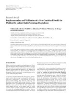
(a) (b) (c)
Figure 1: Observations obtained with background subtraction: (a) reference frame, (b) current frame, and (c) result of background
subtraction (pixels in black are labeled as foreground) and derived object detections (indicated with red bounding boxes).
(a) (b)
Figure 2: Observations obtained with [2] on a water skier sequence
shot by a moving camera: (a) detected moving clusters superposed
on the current frame and (b) mask of pixels characterizing the
observation.
when s ∈ O
(i)
t
∩Ω. As we only consider a sparse motion field,
color distribution only is taken into account for pixels with
no motion vector: p
(i)
t
(z
t
(s)) = p
(i,C)
t
(z
(C)
t
(s)) if s ∈ O
(i)

t
\ Ω.
The background distributions are computed in the same
way. The distribution of the background of object i at time
t,denotedasq
(i)
t
, is a mixture of Gaussians fitted to the set
of values
{z
t
(s)}
s∈P \O
(i)
t
. It also combines motion and color
information:
q
(i)
t

z
t
(s)

= q
(i,C)
t

z

(C)
t
(s)

q
(i,M)
t

z
(M)
t
(s)

. (3)
3.2. Description of the obser vations
Our goal is to perform both segmentation and tracking to get
the object O
(i)
t
corresponding to the object O
(i)
t
−1
of previous
frame. Contrary to sequential segmentation techniques [13,
32, 33], we bring in object-level “observations.” We assume
that, at each time t, there are m
t
observations. The jth,
i

= 1 m
t
, observation at time t is denoted as M
(j)
t
and is
defined as a set of pixels, M
(j)
t
⊂ P .
As objects and backgrounds, observation j at time t
is represented by a distribution, denoted as ρ
(j)
t
,which
is a mixture of Gaussians combining color and motion
information. The mixture is fitted to the set
{z
t
(s)}
s∈M
(j)
t
and
is defined as
ρ
(j)
t

z

t
(s)

=
ρ
(j,C)
t

z
(C)
t
(s)

ρ
(j,M)
t

z
(M)
t
(s)

. (4)
The observations may be of various kinds (e.g., obtained
by a class-specific object detector, or motion/color detec-
tors). Here, we will consider two different types of observa-
tions.
3.2.1. Background subtraction
The first type of observations comes from a preprocessing
step of background subtraction. Each observation amounts

to a connected component of the foreground detection map
obtained by thresholding the difference between a reference
frame and the current frame and by removing small regions
(Figure 1). The connected components are obtained using
the “gap/mountain” method described in [34].
In the first frame, the tracked objects are initialized as the
observations themselves.
3.2.2. Moving objects detection in complex scenes
Inordertobeabletotrackobjectsinmorecomplex
sequences, we will use a second type of objects detector.
The method considered is the one from [2] that can be
decomposed in three main steps. First, a grid G of moving
pixels having valid motion vectors is selected. Each point is
described by its position, its color, and its motion. Then these
points are partitioned based on a mean shift algorithm [35],
leading to several moving clusters. Finally, segmentation
of the objects are obtained from the moving clusters by
minimizing appropriate energy functions with graph cuts.
This last step can be avoided here. Indeed, as we here propose
a method that simultaneously track and segment objects,
the observations do not need to be fully segmented objects.
Therefore, the observations will simply be the detected
clusters of moving points (Figure 2).
The segmentation part of the detection preprocessing
will only be used when initializing new objects to be tracked.
When the system declares that a new tracker should be
created from a given observation, the tracker is initialized
with the corresponding segmented detected object.
In this detection method, motion vectors are only
computed on the points of sparse grid G. Therefore, in our

tracking algorithm, when using this type of observations,
we will stick to this sparse grid as the set of pixels that are
described both by their color and by their motion (Ω
= G).
A. Bugeau and P. P
´
erez 5
Instant t − 1 Instant t
1st example
2nd example
Object 1 Object 2 Object 1
Object 1
Figure 3: Example illustrating why the objects are tracked indepen-
dently.
4. PRINCIPLES OF THE TRACK AND CUT SYSTEM
Before getting to the details of our approach, we start by pre-
senting its main principles. In particular, we explain why it
is decomposed into two steps (first a segmentation/tracking
method and then, when necessary, a further segmentation
step) and why each object is tracked independently.
4.1. Tracking each object independently
We propose in this work a tracking method that is based
on energy minimizations. Minimizing an energy with min-
cut/max-flow in capacity graphs [36] permits to assign a label
to each pixel of an image. As in [37], the labeling of one
pixel will here depend both on the agreement between the
appearance at this pixel and the objects appearances and on
the similarity between this pixel and its neighbors. Indeed,
a binary smoothness term that encourages two neighboring
pixels with similar appearances to get the same label is added

to the energy function.
In our tracking scheme, we wish to assign a label corre-
sponding to one of the tracked objects or to the background
to each pixel of the image. By using a multilabel energy
function (each label corresponding to one object), all objects
would be directly tracked simultaneously by minimizing
a single energy function. However, we prefer not to use
such a multilabel energy in general, and track each object
independently. Such a choice comes from an attempt to dis-
tinguish the merging of several objects from the occlusions of
some objects by another one, which cannot be done using a
multilabel energy function. Let us illustrate this problem on
an example. Assume two objects having similar appearances
are tracked. We are going to analyze and compare the two
following scenarios (described in Figure 3).
On the one hand, we suppose that the two objects
become connected in the image plane at time t and, on the
other hand, that one of the objects occludes the second one
at time t.
First, suppose that these two objects are tracked using
a multilabel energy function. Since the appearances of the
objects are similar, when they get side by side (first case),
the minimization will tend to label all the pixels in the
same way (due to the smoothness term). Hence, each pixel
will probably be assigned the same label, corresponding to
only one of the tracked objects. In the second case, when
one object occludes the other one, the energy minimization
leads to the same result: all the pixels have the same
label. Therefore, it is possible for these two scenarios to be
confused.

Assume now that each object is tracked independently by
defining one energy function per object (each pixel is then
associated to k
t−1
labels). For each object, the final label of
a pixel is either “object” or “background.” For the first case,
each pixel of the two objects will be, at the end of the two
minimizations, labeled as “object.” For the second case, the
pixels will be labeled as “object” when the minimization is
done for the occluding object and as “background” for the
occluded one. Therefore, by defining one energy function per
object, we are able to differentiate the two cases. Of course,
for the first case, the obtained result is not the wanted one:
the pixels get the same label which means that the two objects
have merged. In order to keep distinguishing the two objects,
we equip our tracking system with an additional separation
step in case objects get merged.
The principles of the tracking, including the separation
of merged objects, are explained in next subsections.
4.2. Principle of the tracking method
The principle of our algorithm is as follows. A prediction
O
(i)
t
|t−1
⊂ P is made for each object i of time t − 1. We denote
as d
(i)
t
−1

the mean, over all pixels of the object at time t − 1, of
optical flow values:
d
(i)
t
−1
=

s∈O
(i)
t
−1
∩Ω
z
(M)
t
−1
(s)


O
(i)
t
−1
∩ Ω


. (5)
The prediction is obtained by translating each pixel belong-
ing to O

(i)
t
−1
bythisaverageopticalflow:
O
(i)
t
|t−1
=

s + d
(i)
t
−1
, s ∈ O
(i)
t
−1

. (6)
Using this prediction, the new observations and the
distribution p
(i)
t
of O
(i)
t
−1
, an energy function is built. This
energy is minimized using min-cut/max-flow algorithm

[36], which gives the new segmented object at time t, O
(i)
t
.
The minimization also provides the correspondences of the
object with all the available observations, which simply leads
to the creation of new trackers when one or several obser-
vations at current instant remain unassociated. Our tracking
algorithm is diagrammatically summarized in Figure 4.
4.3. Separating merged objects
At the end of the tracking step, several objects can be merged,
that is, the segmentations for different objects overlap:
∃(i, j):O
(i)
t
∩O
(j)
t
/
= ∅. In order to keep tracking each object
separately, the merged objects must be separated. This will be
done by adding a multilabel energy minimization.
6 EURASIP Journal on Image and Video Processing
5. ENERGY FUNCTIONS
We define one tracker per object. To each tracker corre-
sponds, for each frame, one graph and one energy function
that is minimized using the min-cut/max-flow algorithm
[36]. Nodes and edges of the graph can be seen in Figure 5.
This figure will be further explained in Section 5.1.Inallour
work, we consider an 8-neighborhood system. However, for

the sake of clarity, only a 4-neighborhood is used in all the
figures representing a graph.
5.1. Graph
The undirected graph G
t
= (V
t
, E
t
)attimet is defined as
asetofnodesV
t
and a set of edges E
t
. The set of nodes is
composed of two subsets. The first subset is the set of the N
pixels of the image grid P. The second subset corresponds to
the observations: to each observation mask M
(j)
t
is associated
anoden
(j)
t
. We call these nodes “observation nodes.” The set
ofnodesthusreadsV
t
= P ∪{n
(j)
t

, j = 1 m
t
}. The set of
edges is decomposed as follows: E
t
= E
P
∪
m
t
j=1
E
M
(j)
t
,whereE
P
is the set of all unordered pairs {s, r} of neighboring elements
of P ,andE
M
(j)
t
is the set of unordered pairs {s, n
(j)
t
},with
s
∈ M
(j)
t

.
Segmenting the object O
(i)
t
amounts to assigning a label
l
(i)
s,t
, either background, ”bg,” or object, “fg,” to each pixel
node s of the graph. Associating observations to tracked
objects amounts to assigning a binary label l
(i)
j,t

“bg” or “fg”)
to each observation node n
(j)
t
(for the sake of clarity, the
notation l
(i)
j,t
has been preferred to l
(i)
n
(j)
t
,t

. The set of all the

node labels is denoted as L
(i)
t
.
5.2. Energy
An energy function is defined for each object i at each instant
t.ItiscomposedofdatatermsR
(i)
s,t
and binary smoothness
terms B
(i)
s,r,t
:
E
(i)
t

L
(i)
t

=

s∈V
t
R
(i)
s,t


l
(i)
s,t

+

{s,r}∈E
t
B
(i)
{s,r},t

1 − δ

l
(i)
s,t
, l
(i)
r,t

,
(7)
where δ is the characteristic function defined as
δ

l
s
, l
r


=
⎧
⎨
⎩
1ifl
s
= l
r
,
0 else.
(8)
In order to simplify the notations, we omit object index i in
the rest of this section.
5.2.1. Data term
The data term only concerns the pixel nodes lying in the
predicted regions and the observation nodes. For all the other
pixel nodes, labeling will only be controlled by the neighbors
Prediction
Observations
O
(i)
t
−1
O
(i)
t
|t−1
O
(i)

t
Creation of new objects
Distributions
computation
Construction of
the graph
Energy minimization
(graph cuts)
Correspondences between O
(i)
t
−1
and the observations
Figure 4: Principle of the algorithm.
Object i at time t − 1
(a)
Graph for object i at time t
n
(1)
t
n
(2)
t
O
(i)
t
|t−1
(b)
Figure 5: Description of the graph. The left figure is the result of the
energy minimization at time t

−1. White nodes are labeled as object
and black nodes as background. The optical flow vectors for the
object are shown in blue. The right figure shows the graph at time t.
Two observations are available, each of which giving rise to a special
“observation” node. The pixel nodes circled in red correspond to
the masks of these two observations. The dashed box indicates the
predicted mask.
via binary terms. More precisely, the first part of energy in
(7)reads

s∈V
t
R
s,t

l
s,t

=
α
1

s∈O
t|t−1
− ln

p
1

s, l

s,t

+ α
2
m
t

j=1
d
2

n
(j)
t
, l
j,t

.
(9)
Segmented object at time t should be similar, in terms
of motion and color, to the preceding instance of this object
at time t
− 1. To exploit this consistency assumption, the
distribution of the object, p
t−1
(2),andofthebackground,
q
t−1
(3), from previous image, is used to define the likelihood
p

1
, within predicted region as
p
1
(s, l) =
⎧
⎨
⎩
p
t−1

z
t
(s)

if l = “fg,”
q
t−1

z
t
(s)

if l = “bg.”
(10)
In the same way, an observation should be used only if
it is likely to correspond to the tracked object. To evaluate
the similarity of observation j at time t and object i at
previous time, a comparison between the distributions p
t−1

A. Bugeau and P. P
´
erez 7
and ρ
(j)
t
(4) and between q
t−1
and ρ
(j)
t
must be performed
through the computation of a distance measure. A classical
distance to compare two mixtures of Gaussians, G
1
and G
2
,
is the Kullback-Leibler divergence [38], defined as
KL

G
1
, G
2

=

G
1

(x)log
G
1
(x)
G
2
(x)
dx. (11)
This asymmetric function measures how well distribution
G
2
mimics the variations of distribution G
1
.Here,wewant
to know if the observations belongs to the object or to
the background but not the opposite, and therefore we will
measure if one or several observations belong to one object.
The data term d
2
is then
d
2
(s, l) =
⎧
⎪
⎨
⎪
⎩
KL


ρ
(j)
t
, p
t−1

if l = “fg,”
KL

ρ
(j)
t
, q
t−1

if l = “bg.”
(12)
Two constants α
1
and α
2
are included in the data term in
(9) to give more or less influence to the observations. In our
experiments, they were both fixed to 1.
5.2.2. Binary term
Following [37], the binary term between neighboring pairs
of pixels
{s, r} of P is based on color gradients and has the
form
B

{s,r},t
= λ
1
1
dist(s, r)
e
−(z
(C)
t
(s)−z
(C)
t
(r)
2
)/σ
2
T
. (13)
As in [39], the parameter σ
T
is set to σ
T
= 4·(z
(C)
t
(s) −
z
(C)
t
(r))

2
,where· denotes expectation over a box sur-
rounding the object.
For graph edges between one pixel node and one
observation node, the binary term depends on the distance
between the color of the observation and the pixel color.
More precisely, this term discourages the cut of an edge
linking one pixel to an observation node, if this pixel has a
high probability (through its color and motion) to belong
to the corresponding observation. This binary term is then
computed as
B
{s,n
(j)
t
},t
= λ
2
ρ
(j)
t

z
(C)
t
(s)

. (14)
Parameters λ
1

and λ
2
are discussed in the experiments.
5.2.3. Energy minimization
The final labeling of pixels is obtained by minimizing,
with the min-cut/max-flow algorithm proposed in [40], the
energy defined above:

L
(i)
t
= arg min
L
(i)
t
E
(i)
t

L
(i)
t

. (15)
This labeling finally gives the segmentation of the ith object
at time t as
O
(i)
t
=


s ∈ P :

l
(i)
s,t
= “fg”

. (16)
(a) Result of the tracking algorithm.
3 objects have merged
(b) Corresponding graph
Figure 6: Graph example for the segmentation of merged objects.
5.3. Creation of new objects
One advantage of our approach lies in its ability to jointly
manipulate pixel labels and track-to-detection assignment
labels. This allows the system to track and segment the
objects at time t, while establishing the correspondences
between an object currently tracked and all the approxima-
tive candidate objects obtained by detection in the current
frame. If, after the energy minimization for an object i,an
observation node n
(j)
t
is labeled as “fg” (

l
(i)
t, j
= “fg”) it means

that there is a correspondence between the ith object and the
jth observation. Conversely, if the node is labeled as “bg,” the
object and the observation are not associated.
If for all the objects (i
= 1, , k
t−1
), an observation node
is labeled as “bg” (
∀i,

l
(i)
t, j
= “bg”), then the corresponding
observation does not match any object. In this case, a new
object is created and initialized with this observation. The
number of tracked objects becomes k
t
= k
t−1
+ 1, and the
new object is initialized as
O
(k
t
)
t
= M
(j)
t

. (17)
In practice, the creation of a new object will be only
validated, if the new object is associated to at least one
observation at time t + 1, that is, if
∃ j ∈{1, , m
t+1
} such
that

l
(k
t
)
j,t+1
= “fg.”
6. SEGMENTING MERGED OBJECTS
Assume now that the results of the segmentations for differ-
ent objects overlap, that is to say
∃(i, j), O
(i)
t
∩ O
(j)
t
/
= ∅. (18)
In this case, we propose an additional step to determine
whether these segmentation masks truly correspond to the
same object or if they should be separated. At the end of this
step, each pixel must belong to only one object.

Let us introduce the notation
F
=

i ∈

1, , k
t

|∃j
/
= i such that O
(i)
t
∩ O
(j)
t
/
= ∅

.
(19)
Anewgraph

G
t
= (

V
t

,

E
t
) is created, where

V
t
=∪
i∈F
O
(i)
t
and

E
t
is composed of all unordered pairs of neighboring
pixel nodes in

V
t
. An example of such a graph is presented
in Figure 6.
8 EURASIP Journal on Image and Video Processing
(a) (b) (c)
Figure 7: Results on sequence from PETS 2006 (frames 81, 116, 146, 176, 206, and 248): (a) original frames, (b) result of simple background
subtraction and extracted observations, and (c) tracked objects on current frame using the primary and the secondary energy functions.
A. Bugeau and P. P
´

erez 9
The goal is then to assign to each node s of

V
t
alabel
ψ
s
∈ F . Defining

L ={ψ
s
, s ∈

V
t
} the labeling of

V
t
,anew
energy is defined as

E
t
(

L) =

s∈


V
t
− ln

p
3

s, ψ
s

+ λ
3

{s,r}∈

E
t
1
dist(s, r)
e
−(z
(C)
s
−z
(C)
r

2
)/σ

2
3

1 − δ

ψ
s
, ψ
r

.
(20)
The parameter σ
3
is here set as σ
3
= 4·(z
t
(s)
(i,C)
−z
t
(r)
(i,C)
)
2

with the averaging being over i ∈ F and {s, r}∈

E.The

fact that several objects have been merged shows that their
respective feature distributions at previous instant did not
permit to distinguish them. A way to separate them is then
to increase the role of the prediction. This is achieved by
choosing function p
3
as
p
3
(s, ψ) =
⎧
⎨
⎩
p
(ψ)
t
−1

z
t
(s)

if s
/
∈ O
(ψ)
t
|t−1
,
1 otherwise.

(21)
This multilabel energy function is minimized using the
expansion move algorithm [36, 41]. The convergence to
the global optimal solution with this algorithm cannot be
proved. Only the convergence to a locally optimal solution
is guaranteed. Still, in all our experiments, this method
gave satisfactory results. After this minimization, the objects
O
(i)
t
, i ∈ F are updated.
7. EXPERIMENTAL RESULTS
This section presents various results of joint tracking/seg-
mentation, including cases, where merged objects have to
be separated in a second step. First, we will consider a
relatively simple sequence, with static background, in which
the observations are obtained by background subtraction
(Section 3.2.1). Next, the tracking method will be com-
bined to the moving objects detector introduced in [2]
(Section 3.2.2).
7.1. Tracking objects detected with
background subtraction
In this section, tracking results obtained on a sequence
from the PETS 2006 data corpus (sequence 1 camera 4) are
presented. They are followed by an experimental analysis of
the first energy function (7). More precisely, the influence of
each of its four terms (two for the data part and two for the
smoothness part) is shown in the same image.
7.1.1. A first tracking result
We start by demonstrating the validity of the approach,

including its robustness to partial occlusions and its ability
to segment individually objects that were initially merged.
Following [39], the parameter λ
3
was set to 20. However,
parameters λ
1
and λ
2
had to be tuned by hand to get better
results (λ
1
= 10, λ
2
= 2). Also, the number of classes for the
Gaussian mixture models was set to 10.
First results (Figure 7) demonstrate the good behavior
of our algorithm even in the presence of partial occlusions
and of object fusion. Observations, obtained by subtracting
a reference frame (frame 10 shown in Figure 1(a)) to the
current one, are visible in the second column of Figure 7,
the third column contains the segmentation of the objects
with the subsequent use of the second energy function. In
frame 81, two objects are initialized using the observations.
Note that the connected component extracted with the
“gap/mountain” method misses the legs for the person in
the upper right corner. While this has an impact on the
initial segmentation, the legs are recovered in the final
segmentation as soon as the following frame.
Let us also underline the fact that the proposed method

easily deals with the entrance of new objects in the scene.
This result also shows the robustness of our method to partial
occlusions. For example, partial occlusions occur when the
person at the top passes behind the three other ones (frames
176 and 206). Despite the similar color of all the objects, this
is well handled by the method, as the person is still tracked
when the occlusion stops (frame 248).
Finally note that even if from frame 102, the two persons
at the bottom correspond to only one observation and have
a similar appearance (color and motion), our algorithm
tracks each person separately (frames 116, 146) thanks to the
second energy function. In Figure 8, we show in more details
the influence of the second energy function by comparing
the results obtained with and without it. Before frame 102,
the three persons at the bottom generate three distinct
observations, while, passed this instant, they correspond to
only one or two observations. Even if the motions and colors
of the three persons are very close, the use of the second
multilabel energy function allows their separation.
7.1.2. A qualitative analysis of the first energy function
We now propose an analysis of the influence on the results
of each of the four terms of the energy defined in (7). The
weight of each of these terms is controlled by a parameter.
Indeed, we remind that the complete energy function has
been defined as
E
t
(L
t
) =


s∈V
t

α
1

s∈O
t|t−1
− ln

P
1

s, l
s,t

+ α
2
m
t

j=1
d
2

n
(j)
t
, l

j,t


+ λ
1

{s,r}∈E
P
B
{s,r},t

1 − δ

l
s,t
, l
r,t

+ λ
2
m
t

j=1

{s,r}∈E
M
(j)
t
B

{s,r},t

1 − δ

l
s,t
, l
r,t

.
(22)
To show the influence of each term, we successively set
one of the parameters λ
1
, λ
2
, α
1
,andα
2
to zero. The results
on a frame from the PETS sequence are visible on Figure 9.
Figure 9(a) presents the original image, Figure 9(b) presets
the extracted observation after background subtraction, and
10 EURASIP Journal on Image and Video Processing
(a) (b) (c)
Figure 8: Separating merged objects with the secondary minimization (frames 101 and 102): (a) result of simple background subtraction and
extracted observations, (b) segmentations with the first energy functions only, and (c) segmentation after postprocessing with the secondary
energy function.
(a) Original image (b) Extracted observations (c) Tracked object (d) Tracked object if λ

1
= 0
(e) Tracked object if λ
2
= 0 (f) Tracked object if α
1
= 0 (g) Tracked object if α
2
= 0
Figure 9: Influence of each term of the first energy function on the frame 820 of the PETS sequence.
Figure 9(c) presents the tracked object when using the
complete energy equation (22)withλ
1
= 10, λ
2
= 2, α
1
= 1,
and α
2
= 2.
If the parameter λ
1
is equal to zero, it means that
no spatial regularization is applied to the segmentation.
The final mask of the object then only depends on the
probability of each pixel to belong to the object, the
background, and the observations. That is the reason why
the object is not well segmented in Figure 9(d).Ifλ
2

=
0, the observations do not influence the segmentation of
the object. As can been seen in Figure 9(e),itcanlead
to a slight undersegmentation of the object. In the case
that α
2
= 0, the labeling of an observation node only
depends on the labels of the pixels belonging to this
observation. Therefore, this term mainly influences the
association between the observations and the tracked objects.
Nevertheless, as can be seen in Figure 9(g), it also slightly
modifies the mask of a tracked object, and switching it off
might produce an undersegmentation of the object. Finally,
when α
1
= 0, the energy minimization yields to the spatial
regularization of the observation mask thanks to the binary
smoothness term. The mask of the object then stops on the
strong contours but does not take into account the color
and motion of the pixels belonging to the prediction. In
Figure 9(f), this leads to an oversegmentation of the object
compared to the segmentation of the object at previous time
instants.
This experiment illustrates that each term of the energy
function plays a role of its own on the final segmentation of
the tracked objects.
7.2. Tracking objects in complex scenes
We are now showing the behavior of our tracking algo-
rithm when the sequences are more complex (dynamic
background, moving camera, etc.). For each sequence, the

observations are the moving clusters detected with the
method of [2]. In all this subsection, the parameter λ
3
was
set to 20, λ
1
to 10, and λ
2
to 1.
The first result is on a water skier sequence (Figure 10).
For each image, the moving clusters and the masks
of the tracked objects are superimposed on the original
A. Bugeau and P. P
´
erez 11
t = 80
t
= 58
t
= 51
t
= 31
(a)
t = 243
t
= 225
t
= 215
t
= 177

(b)
Figure 10: Results on a water skier sequence. The observations are moving clusters detected with the method in [2]. At each time instant,
the observations are shown in the left image, while the masks of the tracked objects are shown in the right image.
image. The proposed tracking method permits to correctly
track the water skier (or more precisely his wet suit) all
along the sequence, despite fast trajectory changes, drastic
deformations, and moving surroundings. As can be seen
in the figure (e.g., at time 58), the detector sometimes
fails to detect the skier. No observations are available
in these cases. However, by using the prediction of the
object, our method handles well such situations and keeps
tracking and segmenting correctly the skier. This shows
the robustness of the algorithm to missing observations.
However, if some observations are missing for several
consecutive frames, the segmentation can get deteriorated.
Conversely, this means that the incorporation of the obser-
vations produced by the detection module enables to get
better segmentations than when using only predictions. On
several frames, moving clusters are detected in the water.
Nevertheless, no objects are created in concerned areas.
The reason is that the creation of a new object is only
validated, if the new object is associated to at least one
observation in the following frame. This never happened in
the sequence.
We end by showing results on a driver sequence
(Figure 11). The first object detected and tracked is the face.
Once again, tracking this object shows the robustness of our
method to missing observations. Indeed, even if from frame
19, the face does not move and therefore is not detected, the
algorithm keeps tracking and segmenting it correctly until

the driver starts turning it. The most important result on
this sequence is the tracking of the hands. In image 39, the
masks of the two hands are merged: they have a few pixels in
common. The step of segmentation of merged objects is then
applied and allows the correct separation of the two masks,
which permits to keep tracking these two objects separately.
Finally,ascanbeenseenonframe57,ourmethoddealswell
with the exit of an object from the scene.
8. CONCLUSION
In this paper, we have presented a new method that
simultaneously segments and tracks multiple objects in
videos. Predictions along with observations composed of
detected objects are combined in an energy function which
12 EURASIP Journal on Image and Video Processing
t = 35
t
= 29
t
= 16
t
= 13
(a)
t = 63
t
= 57
t
= 43
t
= 39
(b)

Figure 11: Results on a driver sequence. The observations are moving clusters detected with the method in [2]. At each time instant, the
observations are shown in the left image, while the masks of the tracked objects are shown in the right image.
is minimized with graph cuts. The use of graph cuts permits
the segmentation of the objects at a modest computational
cost, leaving the computational bottleneck at the level of the
detection of objects and of the computation of GMMs.
An important novelty is the use of observation nodes
in the graph which gives better segmentations but also
enables the direct association of the tracked objects to the
observations (without adding any association procedure).
The observations used in this paper are obtained firstly by
a simple background subtraction based on a single reference
frame and secondly by a more sophisticated moving object
detector. Note however that any object detection method
could be used as well, with no change to the approach, as
soon as the observations can be represented by a set of pixels.
The proposed method combines the main advantages of
each of the three categories of existing methods presented in
Section 2. It deals with the entrance of new objects in the
scene and the exit of existing ones, as “detect-before-track”
methods do; as silhouette tracking methods, the energy
minimization directly outputs the segmentation mask of the
objects; it allows robust tracking in a wide range of color
videos thanks to the use of global distributions, as with other
kernel tracking algorithms.
As shown in the experiments, the algorithm is robust
to partial occlusions and to missing observations and
does not require accurate observations to provide good
segmentations. Also, several observations can correspond to
one object (water skier sequence) and several objects can

correspond to one observation (PETS sequence). Thanks to
the use of a second multilabel energy function, our method
allows individual tracking and segmentation of objects which
were not distinguished from each other in the first stage.
As we use feature distributions of objects at previous
time to define current energy functions, our method handles
progressive illumination changes but breaks down in extreme
cases of abrupt illumination changes. However, by adding an
external detector of such changes, we could circumvent this
problem by keeping only the prediction and by updating the
reference frame when the abrupt change occurs.
Also, other cues, such as shapes, could probably be
added to improve the results. The problem would then be
to introduce such a global feature into the energy function.
A. Bugeau and P. P
´
erez 13
Asitturnsout,itisdifficult to add a global term in an
energy function that is minimized by graph cuts. Another
solution could be to select a compact characterization of
the shape (e.g., pose parameters [42], ellipse parameters
[43], normalized central moments [44], or some top-down
knowledge [45]) and to add a term such as the face energy
term proposed in [43] into the energy function.
Apart from these rather specific problems, several
research directions are open. One of them concerns the
design of an unifying energy framework that would allow
segmentation and tracking of multiple objects, while pre-
cluding the incorrect merging of similar objects getting close
to each other in the image plane. Another direction of

research concerns the automatic tuning of the parameters,
which remains an open problem in the recent literature on
image labeling (e.g., figure/ground segmentation) with graph
cuts.
REFERENCES
[1] A. Yilmaz, O. Javed, and M. Shah, “Object tracking: a survey,”
ACM Computing Surveys, vol. 38, no. 4, p. 13, 2006.
[2] A. Bugeau and P. P
´
erez, “Detection and segmentation of
moving objects in highly dynamic scenes,” in Proceedings of
the IEEE Computer Society Conference on Computer Vision and
Pattern Recognition (CVPR ’07), pp. 1–8, Minneapolis, Minn,
USA, June 2007.
[3] A. Bugeau and P. P
´
erez, “Track and cut: simultaneous
tracking and segmentation of multiple objects with graph
cuts,” in Proceedings of the 3rd International Conference on
Computer Vision Theory and Applications (VISAPP ’08),pp.
1–8, Madeira, Portugal, January 2008.
[4] R. Kalman, “A new approach to linear filtering and prediction
problems,” Journal of Basic Engineering, vol. 82, pp. 35–45,
1960.
[5]N.J.Gordon,D.J.Salmond,andA.F.M.Smith,“Novel
approach to nonlinear/non-Gaussian Bayesian state estima-
tion,” IEE Proceedings F: Radar and Signal Processing, vol. 140,
no. 2, pp. 107–113, 1993.
[6] D. Reid, “An algorithm for tracking multiple targets,” IEEE
Transactions on Automatic Control, vol. 24, no. 6, pp. 843–854,

1979.
[7] I. J. Cox, “A review of statistical data association techniques for
motion correspondence,” International Journal of Computer
Vision, vol. 10, no. 1, pp. 53–66, 1993.
[8] Y. Bar-Shalom and X. Li, Estimation and Tracking: Principles,
Techniques, and Software, Artech House, Boston, Mass, USA,
1993.
[9] Y. Bar-Shalom and X. Li, Multisensor-Multitarget Tracking:
Principles and Techniques, YBS Publishing, Storrs, Conn, USA,
1995.
[10] D. Terzopoulos and R. Szeliski, “Tracking with Kalman
snakes,” in Active Vision, pp. 3–20, MIT Press, Cambridge,
Mass, USA, 1993.
[11] M. Isard and A. Blake, “Condensation—conditional density
propagation for visual tracking,” International Journal of
Computer Vision, vol. 29, no. 1, pp. 5–28, 1998.
[12] J. MacCormick and A. Blake, “A probabilistic exclusion
principle for tracking multiple objects,” International Journal
of Computer Vision, vol. 39, no. 1, pp. 57–71, 2000.
[13] N. Paragios and R. Deriche, “Geodesic active regions for
motion estimation and tracking,” in Proceedings of the 7th
IEEE International Conference on Computer Vision (ICCV ’99),
vol. 1, pp. 688–694, Kerkyra, Greece, September 1999.
[14] A. Criminisi, G. Cross, A. Blake, and V. Kolmogorov, “Bilayer
segmentation of live video,” in Proceedings of the IEEE
Computer Society Conference on Computer Vision and Pattern
Recognition (CVPR ’06), vol. 1, pp. 53–60, New York, NY, USA,
June 2006.
[15] N. Paragios and G. Tziritas, “Adaptive detection and localiza-
tion of moving objects in image sequences,” Signal Processing:

Image Communication, vol. 14, no. 4, pp. 277–296, 1999.
[16] Y. Shi and W. C. Karl, “Real-time tracking using level sets,”
in Proceedings of the IEEE Computer Society Conference on
Computer Vision and Pattern Recognition (CVPR ’05), vol. 2,
pp. 34–41, San Diego, Calif, USA, June 2005.
[17] M. Bertalmio, G. Sapiro, and G. Randall, “Morphing active
contours,” IEEE Transactions on Pattern Analysis and Machine
Intelligence, vol. 22, no. 7, pp. 733–737, 2000.
[18] D. Cremers and C. Schn
¨
orr, “Statistical shape knowledge in
variational motion segmentation,” Image and Vision Comput-
ing, vol. 21, no. 1, pp. 77–86, 2003.
[19] A R. Mansouri, “Region tracking via level set PDEs without
motion computation,” IEEE Transactions on Pattern Analysis
and Machine Intelligence, vol. 24, no. 7, pp. 947–961, 2002.
[20] R. Ronfard, “Region-based strategies for active contour mod-
els,” International Journal of Computer Vision,vol.13,no.2,
pp. 229–251, 1994.
[21] A. Yilmaz, X. Li, and M. Shah, “Contour-based object tracking
with occlusion handling in video acquired using mobile
cameras,” IEEE Transactions on Pattern Analysis and Machine
Intelligence, vol. 26, no. 11, pp. 1531–1536, 2004.
[22] N. Xu and N. Ahuja, “Object contour tracking using graph
cuts based active contours,” in Proceedings of the IEEE
International Conference on Image Processing (ICIP ’02), vol.
3, pp. 277–280, Rochester, NY, USA, September 2002.
[23] J. Shi and C. Tomasi, “Good features to track,” in Proceedings
of the IEEE Conference on Computer Vision and Pattern
Recognition (CVPR ’94), pp. 593–600, Seattle, Wash, USA,

June 1994.
[24] D. Comaniciu, V. Ramesh, and P. Meer, “Real-time tracking
of non-rigid objects using mean shift,” in Proceedings of the
IEEE Computer Society Conference on Computer Vision and
Pattern Recognition (CVPR ’00), vol. 2, pp. 142–149, Hilton
Head Island, SC, USA, June 2000.
[25] D. Comaniciu, V. Ramesh, and P. Meer, “Kernel-based optical
tracking,” IEEE Transactions on Pattern Analysis and Machine
Intelligence, vol. 25, no. 5, pp. 564–577, 2003.
[26] D. Freedman and M. W. Turek, “Illumination-invariant
tracking via graph cuts,” in Proceedings of the IEEE Computer
Society Conference on Computer Vision and Pattern Recognition
(CVPR ’05) , vol. 2, pp. 10–17, San Diego, Calif, USA, June
2005.
[27] R. Kjeldsen and J. Kender, “Finding skin in color images,” in
Proceedings of the 2nd International Conference on Automatic
Face and Gesture Recognition (FG ’96), pp. 312–317, Killington,
Vt, USA, October 1996.
[28] M. Singh and N. Ahuja, “Regression based bandwidth selec-
tion for segmentation using Parzen windows,” in Proceedings
of the 9th IEEE International Conference on Computer Vision
(ICCV ’03), vol. 1, pp. 2–9, Nice, France, October 2003.
14 EURASIP Journal on Image and Video Processing
[29] B. D. Lucas and T. Kanade, “An iterative technique of image
registration and its application to stereo,” in Proceedings of
the 7th International Joint Conference on Artificial Intelligence
(IJCAI ’81), Vancouver, Canada, August 1981.
[30] A. D. Jepson, D. J. Fleet, and T. F. El-Maraghi, “Robust online
appearance models for visual tracking,” IEEE Transactions on
Pattern Analysis and Machine Intelligence, vol. 25, no. 10, pp.

1296–1311, 2003.
[31] H. T. Nguyen and A. W. M. Smeulders, “Fast occluded object
tracking by a robust appearance filter,” IEEE Transactions on
Pattern Analysis and Machine Intelligence, vol. 26, no. 8, pp.
1099–1104, 2004.
[32] O. Juan and Y. Boykov, “Active graph cuts,” in Proceedings of
the IEEE Computer Society Conference on Computer Vision and
Pattern Recognition (CVPR ’06), vol. 1, pp. 1023–1029, New
York, NY, USA, June 2006.
[33] P. Kohli and P. Torr, “Effciently solving dynamic markov
random fields using graph cuts,” in Proceedings of the 10th
IEEE International Conference on Computer Vision (ICCV ’05),
pp. 922–929, Beijing, China, October 2005.
[34] Y. Wang, J. F. Doherty, and R. E. Van Dyck, “Moving object
tracking in video,” in Proceedings of the 29th Applied Imagery
Pattern Recognition Workshop (AIPR ’00), p. 95, Washington,
DC, USA, October 2000.
[35] D. Comaniciu and P. Meer, “Mean shift: a robust approach
toward feature space analysis,” IEEE Transactions on Pattern
Analysis and Machine Intelligence, vol. 24, no. 5, pp. 603–619,
2002.
[36] Y. Boykov, O. Veksler, and R. Zabih, “Fast approximate energy
minimization via graph cuts,” IEEE Transactions on Pattern
Analysis and Machine Intelligence, vol. 23, no. 11, pp. 1222–
1239, 2001.
[37] Y. Boykov and M P. Jolly, “Interactive graph cuts for optimal
boundary & region segmentation of objects in N-D images,”
in Proceedings of the 8th IEEE International Conference on
Computer Vision (ICCV ’01), vol. 1, pp. 105–112, Vancouver,
Canada, July 2001.

[38] S. Kullback and R. A. Leibler, “On information and suffi-
ciency,” Annals of Mathematical Statistics, vol. 22, no. 1, pp.
79–86, 1951.
[39] A. Blake, C. Rother, M. Brown, P. P
´
erez, and P. Torr,
“Interactive image segmentation using an adaptive GMMRF
model,” in Proceedings of the 8th European Conference on
Computer Vision (ECCV ’04), pp. 428–441, Prague, Czech
Republic, May 2004.
[40] Y. Boykov and V. Kolmogorov, “An experimental comparison
of min-cut/max-flow algorithms for energy minimization in
vision,” IEEE Transactions on Pattern Analysis and Machine
Intelligence, vol. 26, no. 9, pp. 1124–1137, 2004.
[41] Y. Boykov, O. Veksler, and R. Zabih, “Markov random fields
with efficient approximations,” in Proceedings of the IEEE
Computer Society Conference on Computer Vision and Pattern
Recognition (CVPR ’98), pp. 648–655, Santa Barbara, Calif,
USA, June 1998.
[42] M. Bray, P. Kohli, and P. Torr, “PoseCut: simultaneous seg-
mentation and 3D pose estimation of humans using dynamic
graph-cuts,” in Proceedings of the 9th European Conference on
Computer Vision (ECCV ’06), pp. 642–655, Graz, Austria, May
2006.
[43] J. Rihan, P. Kohli, and P. Torr, “Objcut for face detection,” in
Proceedings of the 4th Indian Conference on Computer Vision,
Graphics and Image Processing (ICVGIP ’06), pp. 861–871,
Madurai, India, December 2006.
[44] L. Zhao and L. S. Davis, “Closely coupled object detection and
segmentation,” in Proceedings of the 10th IEEE International

Conference on Computer Vision (ICCV ’05)
, vol. 1, pp. 454–
461, Beijing, China, October 2005.
[45] D. Ramanan, “Using segmentation to verify object hypothe-
ses,” in Proceedings of the IEEE Computer Society Conference
on Computer Vision and Pattern Recognition (CVPR ’07),
Minneapolis, Minn, USA, June 2007.