Introductory business statistics op

Introductory Business
Statistics

SENIOR CONTRIBUTING AUTHORS

ALEXANDER HOLMES, THE UNIVERSITY OF OKLAHOMA
BARBARA ILLOWSKY, DE ANZA COLLEGE
SUSAN DEAN, DE ANZA COLLEGE





OpenStax
Rice University
6100 Main Street MS-375
Houston, Texas 77005
To learn more about OpenStax, visit .
Individual print copies and bulk orders can be purchased through our website.
©2018 Rice University. Textbook content produced by OpenStax is licensed under a Creative Commons
Attribution 4.0 International License (CC BY 4.0). Under this license, any user of this textbook or the textbook
contents herein must provide proper attribution as follows:
-

-

-

-

If you redistribute this textbook in a digital format (including but not limited to PDF and HTML), then you
must retain on every page the following attribution:
“Download for free at />If you redistribute this textbook in a print format, then you must include on every physical page the
following attribution:
“Download for free at />If you redistribute part of this textbook, then you must retain in every digital format page view (including
but not limited to PDF and HTML) and on every physical printed page the following attribution:
“Download for free at />If you use this textbook as a bibliographic reference, please include
in your citation.

For questions regarding this licensing, please contact
Trademarks
The OpenStax name, OpenStax logo, OpenStax book covers, OpenStax CNX name, OpenStax CNX logo,
OpenStax Tutor name, Openstax Tutor logo, Connexions name, Connexions logo, Rice University name, and
Rice University logo are not subject to the license and may not be reproduced without the prior and express
written consent of Rice University.
PRINT BOOK ISBN-10
PRINT BOOK ISBN-13
PDF VERSION ISBN-10
PDF VERSION ISBN-13
Revision Number
Original Publication Year



1-947172-46-8
978-1-947172-46-3
1-947172-47-6

978-1-947172-47-0
IBS-2017-001(03/18)-LC
2017



OPENSTAX

OpenStax provides free, peer-reviewed, openly licensed textbooks for introductory college and Advanced Placement®
courses and low-cost, personalized courseware that helps students learn. A nonprofit ed tech initiative based at Rice
University, we’re committed to helping students access the tools they need to complete their courses and meet their
educational goals.

RICE UNIVERSITY
OpenStax, OpenStax CNX, and OpenStax Tutor are initiatives of Rice University. As a leading research university with a
distinctive commitment to undergraduate education, Rice University aspires to path-breaking research, unsurpassed
teaching, and contributions to the betterment of our world. It seeks to fulfill this mission by cultivating a diverse community
of learning and discovery that produces leaders across the spectrum of human endeavor.

FOUNDATION SUPPORT
OpenStax is grateful for the tremendous support of our sponsors. Without their strong engagement, the goal
of free access to high-quality textbooks would remain just a dream.
Laura and John Arnold Foundation (LJAF) actively seeks opportunities to invest in organizations and
thought leaders that have a sincere interest in implementing fundamental changes that not only
yield immediate gains, but also repair broken systems for future generations. LJAF currently focuses
its strategic investments on education, criminal justice, research integrity, and public accountability.
The William and Flora Hewlett Foundation has been making grants since 1967 to help solve social
and environmental problems at home and around the world. The Foundation concentrates its
resources on activities in education, the environment, global development and population,
performing arts, and philanthropy, and makes grants to support disadvantaged communities in the

San Francisco Bay Area.
Calvin K. Kazanjian was the founder and president of Peter Paul (Almond Joy), Inc. He firmly believed
that the more people understood about basic economics the happier and more prosperous they
would be. Accordingly, he established the Calvin K. Kazanjian Economics Foundation Inc, in 1949 as a
philanthropic, nonpolitical educational organization to support efforts that enhanced economic
understanding.
Guided by the belief that every life has equal value, the Bill & Melinda Gates Foundation works to
help all people lead healthy, productive lives. In developing countries, it focuses on improving
people’s health with vaccines and other life-saving tools and giving them the chance to lift
themselves out of hunger and extreme poverty. In the United States, it seeks to significantly
improve education so that all young people have the opportunity to reach their full potential. Based
in Seattle, Washington, the foundation is led by CEO Jeff Raikes and Co-chair William H. Gates Sr.,
under the direction of Bill and Melinda Gates and Warren Buffett.
The Maxfield Foundation supports projects with potential for high impact in science, education,
sustainability, and other areas of social importance.
Our mission at The Michelson 20MM Foundation is to grow access and success by eliminating
unnecessary hurdles to affordability. We support the creation, sharing, and proliferation of more
effective, more affordable educational content by leveraging disruptive technologies, open
educational resources, and new models for collaboration between for-profit, nonprofit, and public
entities.

The Bill and Stephanie Sick Fund supports innovative projects in the areas of Education, Art, Science
and Engineering.




Study where you want, what
you want, when you want.
When you access College Success in our web view, you can use our new online

highlighting and note-taking features to create your own study guides.
Our books are free and flexible, forever.
Get started at openstax.org/details/books/introductory-business-statistics

Access. The future of education.
openstax.org


Table of Contents
Preface . . . . . . . . . . . . . . . . . . . . . . . . . . . . . . . . . . . . . . . . . . . . . . . . .
Chapter 1: Sampling and Data . . . . . . . . . . . . . . . . . . . . . . . . . . . . . . . . . . . .
1.1 Definitions of Statistics, Probability, and Key Terms . . . . . . . . . . . . . . . . . . . . .
1.2 Data, Sampling, and Variation in Data and Sampling . . . . . . . . . . . . . . . . . . . .
1.3 Levels of Measurement . . . . . . . . . . . . . . . . . . . . . . . . . . . . . . . . . . .
1.4 Experimental Design and Ethics . . . . . . . . . . . . . . . . . . . . . . . . . . . . . . .
Chapter 2: Descriptive Statistics . . . . . . . . . . . . . . . . . . . . . . . . . . . . . . . . . .
2.1 Display Data . . . . . . . . . . . . . . . . . . . . . . . . . . . . . . . . . . . . . . . . .
2.2 Measures of the Location of the Data . . . . . . . . . . . . . . . . . . . . . . . . . . . .
2.3 Measures of the Center of the Data . . . . . . . . . . . . . . . . . . . . . . . . . . . . .
2.4 Sigma Notation and Calculating the Arithmetic Mean . . . . . . . . . . . . . . . . . . . .
2.5 Geometric Mean . . . . . . . . . . . . . . . . . . . . . . . . . . . . . . . . . . . . . . .
2.6 Skewness and the Mean, Median, and Mode . . . . . . . . . . . . . . . . . . . . . . . .
2.7 Measures of the Spread of the Data . . . . . . . . . . . . . . . . . . . . . . . . . . . . .
Chapter 3: Probability Topics . . . . . . . . . . . . . . . . . . . . . . . . . . . . . . . . . . . .
3.1 Terminology . . . . . . . . . . . . . . . . . . . . . . . . . . . . . . . . . . . . . . . . .
3.2 Independent and Mutually Exclusive Events . . . . . . . . . . . . . . . . . . . . . . . . .
3.3 Two Basic Rules of Probability . . . . . . . . . . . . . . . . . . . . . . . . . . . . . . . .
3.4 Contingency Tables and Probability Trees . . . . . . . . . . . . . . . . . . . . . . . . . .
3.5 Venn Diagrams . . . . . . . . . . . . . . . . . . . . . . . . . . . . . . . . . . . . . . . .
Chapter 4: Discrete Random Variables . . . . . . . . . . . . . . . . . . . . . . . . . . . . . . .

4.1 Hypergeometric Distribution . . . . . . . . . . . . . . . . . . . . . . . . . . . . . . . . .
4.2 Binomial Distribution . . . . . . . . . . . . . . . . . . . . . . . . . . . . . . . . . . . . .
4.3 Geometric Distribution . . . . . . . . . . . . . . . . . . . . . . . . . . . . . . . . . . . .
4.4 Poisson Distribution . . . . . . . . . . . . . . . . . . . . . . . . . . . . . . . . . . . . .
Chapter 5: Continuous Random Variables . . . . . . . . . . . . . . . . . . . . . . . . . . . . .
5.1 Properties of Continuous Probability Density Functions . . . . . . . . . . . . . . . . . . .
5.2 The Uniform Distribution . . . . . . . . . . . . . . . . . . . . . . . . . . . . . . . . . . .
5.3 The Exponential Distribution . . . . . . . . . . . . . . . . . . . . . . . . . . . . . . . . .
Chapter 6: The Normal Distribution . . . . . . . . . . . . . . . . . . . . . . . . . . . . . . . . .
6.1 The Standard Normal Distribution . . . . . . . . . . . . . . . . . . . . . . . . . . . . . .
6.2 Using the Normal Distribution . . . . . . . . . . . . . . . . . . . . . . . . . . . . . . . .
6.3 Estimating the Binomial with the Normal Distribution . . . . . . . . . . . . . . . . . . . .
Chapter 7: The Central Limit Theorem . . . . . . . . . . . . . . . . . . . . . . . . . . . . . . .
7.1 The Central Limit Theorem for Sample Means . . . . . . . . . . . . . . . . . . . . . . .
7.2 Using the Central Limit Theorem . . . . . . . . . . . . . . . . . . . . . . . . . . . . . . .
7.3 The Central Limit Theorem for Proportions . . . . . . . . . . . . . . . . . . . . . . . . .
7.4 Finite Population Correction Factor . . . . . . . . . . . . . . . . . . . . . . . . . . . . .
Chapter 8: Confidence Intervals . . . . . . . . . . . . . . . . . . . . . . . . . . . . . . . . . . .
8.1 A Confidence Interval for a Population Standard Deviation, Known or Large Sample Size .
8.2 A Confidence Interval for a Population Standard Deviation Unknown, Small Sample Case .
8.3 A Confidence Interval for A Population Proportion . . . . . . . . . . . . . . . . . . . . . .
8.4 Calculating the Sample Size n: Continuous and Binary Random Variables . . . . . . . . .
Chapter 9: Hypothesis Testing with One Sample . . . . . . . . . . . . . . . . . . . . . . . . . .
9.1 Null and Alternative Hypotheses . . . . . . . . . . . . . . . . . . . . . . . . . . . . . . .
9.2 Outcomes and the Type I and Type II Errors . . . . . . . . . . . . . . . . . . . . . . . . .
9.3 Distribution Needed for Hypothesis Testing . . . . . . . . . . . . . . . . . . . . . . . . .
9.4 Full Hypothesis Test Examples . . . . . . . . . . . . . . . . . . . . . . . . . . . . . . .
Chapter 10: Hypothesis Testing with Two Samples . . . . . . . . . . . . . . . . . . . . . . . .
10.1 Comparing Two Independent Population Means . . . . . . . . . . . . . . . . . . . . . .
10.2 Cohen's Standards for Small, Medium, and Large Effect Sizes . . . . . . . . . . . . . .

10.3 Test for Differences in Means: Assuming Equal Population Variances . . . . . . . . . . .
10.4 Comparing Two Independent Population Proportions . . . . . . . . . . . . . . . . . . .
10.5 Two Population Means with Known Standard Deviations . . . . . . . . . . . . . . . . .
10.6 Matched or Paired Samples . . . . . . . . . . . . . . . . . . . . . . . . . . . . . . . .
Chapter 11: The Chi-Square Distribution . . . . . . . . . . . . . . . . . . . . . . . . . . . . . .
11.1 Facts About the Chi-Square Distribution . . . . . . . . . . . . . . . . . . . . . . . . . .

.
.
.
.
.
.
.
.
.
.
.
.
.
.
.
.
.
.
.
.
.
.
.

.
.
.
.
.
.
.
.
.
.
.
.
.
.
.
.
.
.
.
.
.
.
.
.
.
.
.
.
.
.

.
.
.
.

.
.
.
.

1
5
5
8
21
29
45
46
64
71
75
76
77
79
133
133
138
146
151
163

203
205
206
209
214
241
242
246
249
279
280
282
289
307
308
310
318
320
333
334
343
346
350
381
382
383
386
392
419
420

427
428
429
432
435
465
466


11.2 Test of a Single Variance . . . . . . . . . . . . . . . . . . . . . . . . . . . . . . .
11.3 Goodness-of-Fit Test . . . . . . . . . . . . . . . . . . . . . . . . . . . . . . . . .
11.4 Test of Independence . . . . . . . . . . . . . . . . . . . . . . . . . . . . . . . . .
11.5 Test for Homogeneity . . . . . . . . . . . . . . . . . . . . . . . . . . . . . . . . .
11.6 Comparison of the Chi-Square Tests . . . . . . . . . . . . . . . . . . . . . . . . .
Chapter 12: F Distribution and One-Way ANOVA . . . . . . . . . . . . . . . . . . . . . . .
12.1 Test of Two Variances . . . . . . . . . . . . . . . . . . . . . . . . . . . . . . . . .
12.2 One-Way ANOVA . . . . . . . . . . . . . . . . . . . . . . . . . . . . . . . . . . .
12.3 The F Distribution and the F-Ratio . . . . . . . . . . . . . . . . . . . . . . . . . .
12.4 Facts About the F Distribution . . . . . . . . . . . . . . . . . . . . . . . . . . . .
Chapter 13: Linear Regression and Correlation . . . . . . . . . . . . . . . . . . . . . . .
13.1 The Correlation Coefficient r . . . . . . . . . . . . . . . . . . . . . . . . . . . . .
13.2 Testing the Significance of the Correlation Coefficient . . . . . . . . . . . . . . . .
13.3 Linear Equations . . . . . . . . . . . . . . . . . . . . . . . . . . . . . . . . . . .
13.4 The Regression Equation . . . . . . . . . . . . . . . . . . . . . . . . . . . . . . .
13.5 Interpretation of Regression Coefficients: Elasticity and Logarithmic Transformation
13.6 Predicting with a Regression Equation . . . . . . . . . . . . . . . . . . . . . . . .
13.7 How to Use Microsoft Excel® for Regression Analysis . . . . . . . . . . . . . . . .
Appendix A: Statistical Tables . . . . . . . . . . . . . . . . . . . . . . . . . . . . . . . . .
Appendix B: Mathematical Phrases, Symbols, and Formulas . . . . . . . . . . . . . . . .
Index . . . . . . . . . . . . . . . . . . . . . . . . . . . . . . . . . . . . . . . . . . . . . . .

This OpenStax book is available for free at />
.
.
.
.
.
.
.
.
.
.
.
.
.
.
.
.
.
.
.
.
.

.
.
.
.
.
.

.
.
.
.
.
.
.
.
.
.
.
.
.
.
.

.
.
.
.
.
.
.
.
.
.
.
.
.
.

.
.
.
.
.
.
.

.
.
.
.
.
.
.
.
.
.
.
.
.
.
.
.
.
.
.
.
.

466
470
477
482
485
513
513
517
517
526
551
552
555
556
558
571
574
577
595
613
621


Preface

1

PREFACE
Welcome to Introductory Business Statistics, an OpenStax resource. This textbook was written to increase student access to
high-quality learning materials, maintaining highest standards of academic rigor at little to no cost.

About OpenStax
OpenStax is a nonprofit based at Rice University, and it’s our mission to improve student access to education. Our first
openly licensed college textbook was published in 2012, and our library has since scaled to over 25 books for college
and AP® courses used by hundreds of thousands of students. OpenStax Tutor, our low-cost personalized learning tool, is
being used in college courses throughout the country. Through our partnerships with philanthropic foundations and our
alliance with other educational resource organizations, OpenStax is breaking down the most common barriers to learning
and empowering students and instructors to succeed.

About OpenStax resources
Customization
Introductory Business Statistics is licensed under a Creative Commons Attribution 4.0 International (CC BY) license, which
means that you can distribute, remix, and build upon the content, as long as you provide attribution to OpenStax and its
content contributors.
Because our books are openly licensed, you are free to use the entire book or pick and choose the sections that are most
relevant to the needs of your course. Feel free to remix the content by assigning your students certain chapters and sections
in your syllabus, in the order that you prefer. You can even provide a direct link in your syllabus to the sections in the web
view of your book.
Instructors also have the option of creating a customized version of their OpenStax book. The custom version can be made
available to students in low-cost print or digital form through their campus bookstore. Visit the Instructor Resources section
of your book page on OpenStax.org for more information.

Errata
All OpenStax textbooks undergo a rigorous review process. However, like any professional-grade textbook, errors
sometimes occur. Since our books are web based, we can make updates periodically when deemed pedagogically necessary.
If you have a correction to suggest, submit it through the link on your book page on OpenStax.org. Subject matter experts
review all errata suggestions. OpenStax is committed to remaining transparent about all updates, so you will also find a list
of past errata changes on your book page on OpenStax.org.

Format

You can access this textbook for free in web view or PDF through OpenStax.org, and for a low cost in print.

About Introductory Business Statistics
Introductory Business Statistics is designed to meet the scope and sequence requirements of the one-semester statistics
course for business, economics, and related majors. Core statistical concepts and skills have been augmented with practical
business examples, scenarios, and exercises. The result is a meaningful understanding of the discipline which will serve
students in their business careers and real-world experiences.

Coverage and scope
Introductory Business Statistics began as a customized version of OpenStax Introductory Statistics by Barbara Illowsky and
Susan Dean. Statistics faculty at The University of Oklahoma have used the business statistics adaptation for several years,
and the author has continually refined it based on student success and faculty feedback.
The book is structured in a similar manner to most traditional statistics textbooks. The most significant topical changes
occur in the latter chapters on regression analysis. Discrete probability density functions have been reordered to provide a
logical progression from simple counting formulas to more complex continuous distributions. Many additional homework
assignments have been added, as well as new, more mathematical examples.
Introductory Business Statistics places a significant emphasis on the development and practical application of formulas so
that students have a deeper understanding of their interpretation and application of data. To achieve this unique approach,
the author included a wealth of additional material and purposely de-emphasized the use of the scientific calculator. Specific
changes regarding formula use include:


2

Preface

• Expanded discussions of the combinatorial formulas, factorials, and sigma notation
• Adjustments to explanations of the acceptance/rejection rule for hypothesis testing, as well as a focus on terminology
regarding confidence intervals
• Deep reliance on statistical tables for the process of finding probabilities (which would not be required if probabilities

relied on scientific calculators)
• Continual and emphasized links to the Central Limit Theorem throughout the book; Introductory Business Statistics
consistently links each test statistic back to this fundamental theorem in inferential statistics
Another fundamental focus of the book is the link between statistical inference and the scientific method. Business and
economics models are fundamentally grounded in assumed relationships of cause and effect. They are developed to both
test hypotheses and to predict from such models. This comes from the belief that statistics is the gatekeeper that allows
some theories to remain and others to be cast aside for a new perspective of the world around us. This philosophical view is
presented in detail throughout and informs the method of presenting the regression model, in particular.
The correlation and regression chapter includes confidence intervals for predictions, alternative mathematical forms to allow
for testing categorical variables, and the presentation of the multiple regression model.

Pedagogical features
• Examples are placed strategically throughout the text to show students the step-by-step process of interpreting and
solving statistical problems. To keep the text relevant for students, the examples are drawn from a broad spectrum of
practical topics; these include examples about college life and learning, health and medicine, retail and business, and
sports and entertainment.
• Practice, Homework, and Bringing It Together give the students problems at various degrees of difficulty while
also including real-world scenarios to engage students.

Additional resources
Student and instructor resources
We’ve compiled additional resources for both students and instructors, including Getting Started Guides, an instructor
solution manual, and PowerPoint slides. Instructor resources require a verified instructor account, which you can apply for
when you log in or create your account on OpenStax.org. Take advantage of these resources to supplement your OpenStax
book.

Community Hubs
OpenStax partners with the Institute for the Study of Knowledge Management in Education (ISKME) to offer Community
Hubs on OER Commons – a platform for instructors to share community-created resources that support OpenStax books,
free of charge. Through our Community Hubs, instructors can upload their own materials or download resources to use

in their own courses, including additional ancillaries, teaching material, multimedia, and relevant course content. We
encourage instructors to join the hubs for the subjects most relevant to your teaching and research as an opportunity both to
enrich your courses and to engage with other faculty.
To reach the Community Hubs, visit www.oercommons.org/hubs/OpenStax.

Technology partners
As allies in making high-quality learning materials accessible, our technology partners offer optional low-cost tools that are
integrated with OpenStax books. To access the technology options for your text, visit your book page on OpenStax.org.

About the authors
Senior contributing authors
Alexander Holmes, The University of Oklahoma
Barbara Illowsky, DeAnza College
Susan Dean, DeAnza College

Contributing authors
Kevin Hadley, Analyst, Federal Reserve Bank of Kansas City

Reviewers
Birgit Aquilonius, West Valley College
Charles Ashbacher, Upper Iowa University - Cedar Rapids
Abraham Biggs, Broward Community College

This OpenStax book is available for free at />

Preface

Daniel Birmajer, Nazareth College
Roberta Bloom, De Anza College
Bryan Blount, Kentucky Wesleyan College

Ernest Bonat, Portland Community College
Sarah Boslaugh, Kennesaw State University
David Bosworth, Hutchinson Community College
Sheri Boyd, Rollins College
George Bratton, University of Central Arkansas
Franny Chan, Mt. San Antonio College
Jing Chang, College of Saint Mary
Laurel Chiappetta, University of Pittsburgh
Lenore Desilets, De Anza College
Matthew Einsohn, Prescott College
Ann Flanigan, Kapiolani Community College
David French, Tidewater Community College
Mo Geraghty, De Anza College
Larry Green, Lake Tahoe Community College
Michael Greenwich, College of Southern Nevada
Inna Grushko, De Anza College
Valier Hauber, De Anza College
Janice Hector, De Anza College
Jim Helmreich, Marist College
Robert Henderson, Stephen F. Austin State University
Mel Jacobsen, Snow College
Mary Jo Kane, De Anza College
John Kagochi, University of Houston - Victoria
Lynette Kenyon, Collin County Community College
Charles Klein, De Anza College
Alexander Kolovos
Sheldon Lee, Viterbo University
Sara Lenhart, Christopher Newport University
Wendy Lightheart, Lane Community College
Vladimir Logvenenko, De Anza College

Jim Lucas, De Anza College
Suman Majumdar, University of Connecticut
Lisa Markus, De Anza College
Miriam Masullo, SUNY Purchase
Diane Mathios, De Anza College
Robert McDevitt, Germanna Community College
John Migliaccio, Fordham University
Mark Mills, Central College
Cindy Moss, Skyline College
Nydia Nelson, St. Petersburg College
Benjamin Ngwudike, Jackson State University
Jonathan Oaks, Macomb Community College
Carol Olmstead, De Anza College
Barbara A. Osyk, The University of Akron
Adam Pennell, Greensboro College
Kathy Plum, De Anza College
Lisa Rosenberg, Elon University
Sudipta Roy, Kankakee Community College
Javier Rueda, De Anza College
Yvonne Sandoval, Pima Community College
Rupinder Sekhon, De Anza College
Travis Short, St. Petersburg College
Frank Snow, De Anza College
Abdulhamid Sukar, Cameron University
Jeffery Taub, Maine Maritime Academy
Mary Teegarden, San Diego Mesa College

3

4

John Thomas, College of Lake County
Philip J. Verrecchia, York College of Pennsylvania
Dennis Walsh, Middle Tennessee State University
Cheryl Wartman, University of Prince Edward Island
Carol Weideman, St. Petersburg College
Kyle S. Wells, Dixie State University
Andrew Wiesner, Pennsylvania State University

This OpenStax book is available for free at />
Preface


Chapter 1 | Sampling and Data

5

1 | SAMPLING AND DATA

Figure 1.1 We encounter statistics in our daily lives more often than we probably realize and from many different
sources, like the news. (credit: David Sim)

Introduction
You are probably asking yourself the question, "When and where will I use statistics?" If you read any newspaper, watch
television, or use the Internet, you will see statistical information. There are statistics about crime, sports, education,
politics, and real estate. Typically, when you read a newspaper article or watch a television news program, you are given
sample information. With this information, you may make a decision about the correctness of a statement, claim, or "fact."
Statistical methods can help you make the "best educated guess."
Since you will undoubtedly be given statistical information at some point in your life, you need to know some techniques

for analyzing the information thoughtfully. Think about buying a house or managing a budget. Think about your chosen
profession. The fields of economics, business, psychology, education, biology, law, computer science, police science, and
early childhood development require at least one course in statistics.
Included in this chapter are the basic ideas and words of probability and statistics. You will soon understand that statistics
and probability work together. You will also learn how data are gathered and what "good" data can be distinguished from
"bad."

1.1 | Definitions of Statistics, Probability, and Key Terms
The science of statistics deals with the collection, analysis, interpretation, and presentation of data. We see and use data in
our everyday lives.
In this course, you will learn how to organize and summarize data. Organizing and summarizing data is called descriptive
statistics. Two ways to summarize data are by graphing and by using numbers (for example, finding an average). After you
have studied probability and probability distributions, you will use formal methods for drawing conclusions from "good"
data. The formal methods are called inferential statistics. Statistical inference uses probability to determine how confident
we can be that our conclusions are correct.
Effective interpretation of data (inference) is based on good procedures for producing data and thoughtful examination
of the data. You will encounter what will seem to be too many mathematical formulas for interpreting data. The goal
of statistics is not to perform numerous calculations using the formulas, but to gain an understanding of your data. The
calculations can be done using a calculator or a computer. The understanding must come from you. If you can thoroughly
grasp the basics of statistics, you can be more confident in the decisions you make in life.


6

Chapter 1 | Sampling and Data

Probability
Probability is a mathematical tool used to study randomness. It deals with the chance (the likelihood) of an event occurring.
For example, if you toss a fair coin four times, the outcomes may not be two heads and two tails. However, if you toss
the same coin 4,000 times, the outcomes will be close to half heads and half tails. The expected theoretical probability of

heads in any one toss is 1 or 0.5. Even though the outcomes of a few repetitions are uncertain, there is a regular pattern

2

of outcomes when there are many repetitions. After reading about the English statistician Karl Pearson who tossed a coin
24,000 times with a result of 12,012 heads, one of the authors tossed a coin 2,000 times. The results were 996 heads. The
fraction 996 is equal to 0.498 which is very close to 0.5, the expected probability.

2000

The theory of probability began with the study of games of chance such as poker. Predictions take the form of probabilities.
To predict the likelihood of an earthquake, of rain, or whether you will get an A in this course, we use probabilities. Doctors
use probability to determine the chance of a vaccination causing the disease the vaccination is supposed to prevent. A
stockbroker uses probability to determine the rate of return on a client's investments. You might use probability to decide to
buy a lottery ticket or not. In your study of statistics, you will use the power of mathematics through probability calculations
to analyze and interpret your data.

Key Terms
In statistics, we generally want to study a population. You can think of a population as a collection of persons, things, or
objects under study. To study the population, we select a sample. The idea of sampling is to select a portion (or subset)
of the larger population and study that portion (the sample) to gain information about the population. Data are the result of
sampling from a population.
Because it takes a lot of time and money to examine an entire population, sampling is a very practical technique. If you
wished to compute the overall grade point average at your school, it would make sense to select a sample of students who
attend the school. The data collected from the sample would be the students' grade point averages. In presidential elections,
opinion poll samples of 1,000–2,000 people are taken. The opinion poll is supposed to represent the views of the people
in the entire country. Manufacturers of canned carbonated drinks take samples to determine if a 16 ounce can contains 16
ounces of carbonated drink.
From the sample data, we can calculate a statistic. A statistic is a number that represents a property of the sample. For
example, if we consider one math class to be a sample of the population of all math classes, then the average number of

points earned by students in that one math class at the end of the term is an example of a statistic. The statistic is an estimate
of a population parameter, in this case the mean. A parameter is a numerical characteristic of the whole population that
can be estimated by a statistic. Since we considered all math classes to be the population, then the average number of points
earned per student over all the math classes is an example of a parameter.
One of the main concerns in the field of statistics is how accurately a statistic estimates a parameter. The accuracy really
depends on how well the sample represents the population. The sample must contain the characteristics of the population
in order to be a representative sample. We are interested in both the sample statistic and the population parameter in
inferential statistics. In a later chapter, we will use the sample statistic to test the validity of the established population
parameter.
A variable, or random variable, usually notated by capital letters such as X and Y, is a characteristic or measurement that
can be determined for each member of a population. Variables may be numerical or categorical. Numerical variables
take on values with equal units such as weight in pounds and time in hours. Categorical variables place the person or
thing into a category. If we let X equal the number of points earned by one math student at the end of a term, then X is a
numerical variable. If we let Y be a person's party affiliation, then some examples of Y include Republican, Democrat, and
Independent. Y is a categorical variable. We could do some math with values of X (calculate the average number of points
earned, for example), but it makes no sense to do math with values of Y (calculating an average party affiliation makes no
sense).
Data are the actual values of the variable. They may be numbers or they may be words. Datum is a single value.
Two words that come up often in statistics are mean and proportion. If you were to take three exams in your math classes
and obtain scores of 86, 75, and 92, you would calculate your mean score by adding the three exam scores and dividing by
three (your mean score would be 84.3 to one decimal place). If, in your math class, there are 40 students and 22 are men
and 18 are women, then the proportion of men students is 22 and the proportion of women students is 18 . Mean and

40

proportion are discussed in more detail in later chapters.

This OpenStax book is available for free at />
40

Chapter 1 | Sampling and Data

NOTE
The words " mean" and " average" are often used interchangeably. The substitution of one word for the other is
common practice. The technical term is "arithmetic mean," and "average" is technically a center location. However, in
practice among non-statisticians, "average" is commonly accepted for "arithmetic mean."

Example 1.1
Determine what the key terms refer to in the following study. We want to know the average (mean) amount
of money first year college students spend at ABC College on school supplies that do not include books. We
randomly surveyed 100 first year students at the college. Three of those students spent $150, $200, and $225,
respectively.
Solution 1.1
The population is all first year students attending ABC College this term.
The sample could be all students enrolled in one section of a beginning statistics course at ABC College (although
this sample may not represent the entire population).
The parameter is the average (mean) amount of money spent (excluding books) by first year college students at
ABC College this term: the population mean.
The statistic is the average (mean) amount of money spent (excluding books) by first year college students in the
sample.
The variable could be the amount of money spent (excluding books) by one first year student. Let X = the amount
of money spent (excluding books) by one first year student attending ABC College.
The data are the dollar amounts spent by the first year students. Examples of the data are $150, $200, and $225.

1.1

Determine what the key terms refer to in the following study. We want to know the average (mean) amount of
money spent on school uniforms each year by families with children at Knoll Academy. We randomly survey 100
families with children in the school. Three of the families spent $65, $75, and $95, respectively.

Example 1.2
Determine what the key terms refer to in the following study.
A study was conducted at a local college to analyze the average cumulative GPA’s of students who graduated last
year. Fill in the letter of the phrase that best describes each of the items below.
1. Population ____ 2. Statistic ____ 3. Parameter ____ 4. Sample ____ 5. Variable ____ 6. Data ____
a) all students who attended the college last year
b) the cumulative GPA of one student who graduated from the college last year
c) 3.65, 2.80, 1.50, 3.90
d) a group of students who graduated from the college last year, randomly selected
e) the average cumulative GPA of students who graduated from the college last year
f) all students who graduated from the college last year
g) the average cumulative GPA of students in the study who graduated from the college last year
Solution 1.2
1. f; 2. g; 3. e; 4. d; 5. b; 6. c

7


8

Chapter 1 | Sampling and Data

Example 1.3
Determine what the key terms refer to in the following study.
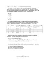
As part of a study designed to test the safety of automobiles, the National Transportation Safety Board collected
and reviewed data about the effects of an automobile crash on test dummies. Here is the criterion they used:
Speed at which Cars Crashed Location of “drive” (i.e. dummies)
35 miles/hour

Front Seat

Table 1.1

Cars with dummies in the front seats were crashed into a wall at a speed of 35 miles per hour. We want to know
the proportion of dummies in the driver’s seat that would have had head injuries, if they had been actual drivers.
We start with a simple random sample of 75 cars.
Solution 1.3
The population is all cars containing dummies in the front seat.
The sample is the 75 cars, selected by a simple random sample.
The parameter is the proportion of driver dummies (if they had been real people) who would have suffered head
injuries in the population.
The statistic is proportion of driver dummies (if they had been real people) who would have suffered head injuries
in the sample.
The variable X = the number of driver dummies (if they had been real people) who would have suffered head
injuries.
The data are either: yes, had head injury, or no, did not.

Example 1.4
Determine what the key terms refer to in the following study.
An insurance company would like to determine the proportion of all medical doctors who have been involved in
one or more malpractice lawsuits. The company selects 500 doctors at random from a professional directory and
determines the number in the sample who have been involved in a malpractice lawsuit.
Solution 1.4
The population is all medical doctors listed in the professional directory.
The parameter is the proportion of medical doctors who have been involved in one or more malpractice suits in
the population.
The sample is the 500 doctors selected at random from the professional directory.
The statistic is the proportion of medical doctors who have been involved in one or more malpractice suits in the
sample.

The variable X = the number of medical doctors who have been involved in one or more malpractice suits.
The data are either: yes, was involved in one or more malpractice lawsuits, or no, was not.

1.2 | Data, Sampling, and Variation in Data and Sampling
Data may come from a population or from a sample. Lowercase letters like x or y generally are used to represent data

This OpenStax book is available for free at />

Chapter 1 | Sampling and Data

9

values. Most data can be put into the following categories:
• Qualitative
• Quantitative
Qualitative data are the result of categorizing or describing attributes of a population. Qualitative data are also often
called categorical data. Hair color, blood type, ethnic group, the car a person drives, and the street a person lives on are
examples of qualitative(categorical) data. Qualitative(categorical) data are generally described by words or letters. For
instance, hair color might be black, dark brown, light brown, blonde, gray, or red. Blood type might be AB+, O-, or B+.
Researchers often prefer to use quantitative data over qualitative(categorical) data because it lends itself more easily to
mathematical analysis. For example, it does not make sense to find an average hair color or blood type.
Quantitative data are always numbers. Quantitative data are the result of counting or measuring attributes of a population.
Amount of money, pulse rate, weight, number of people living in your town, and number of students who take statistics are
examples of quantitative data. Quantitative data may be either discrete or continuous.
All data that are the result of counting are called quantitative discrete data. These data take on only certain numerical
values. If you count the number of phone calls you receive for each day of the week, you might get values such as zero, one,
two, or three.
Data that are not only made up of counting numbers, but that may include fractions, decimals, or irrational numbers, are
called quantitative continuous data. Continuous data are often the results of measurements like lengths, weights, or times.
A list of the lengths in minutes for all the phone calls that you make in a week, with numbers like 2.4, 7.5, or 11.0, would

be quantitative continuous data.

Example 1.5 Data Sample of Quantitative Discrete Data
The data are the number of books students carry in their backpacks. You sample five students. Two students carry
three books, one student carries four books, one student carries two books, and one student carries one book. The
numbers of books (three, four, two, and one) are the quantitative discrete data.

1.5 The data are the number of machines in a gym. You sample five gyms. One gym has 12 machines, one gym has
15 machines, one gym has ten machines, one gym has 22 machines, and the other gym has 20 machines. What type of
data is this?

Example 1.6 Data Sample of Quantitative Continuous Data
The data are the weights of backpacks with books in them. You sample the same five students. The weights (in
pounds) of their backpacks are 6.2, 7, 6.8, 9.1, 4.3. Notice that backpacks carrying three books can have different
weights. Weights are quantitative continuous data.

1.6

The data are the areas of lawns in square feet. You sample five houses. The areas of the lawns are 144 sq. feet,
160 sq. feet, 190 sq. feet, 180 sq. feet, and 210 sq. feet. What type of data is this?


10

Chapter 1 | Sampling and Data

Example 1.7
You go to the supermarket and purchase three cans of soup (19 ounces) tomato bisque, 14.1 ounces lentil, and 19
ounces Italian wedding), two packages of nuts (walnuts and peanuts), four different kinds of vegetable (broccoli,
cauliflower, spinach, and carrots), and two desserts (16 ounces pistachio ice cream and 32 ounces chocolate chip

cookies).
Name data sets that are quantitative discrete, quantitative continuous, and qualitative(categorical).
Solution 1.7
One Possible Solution:
• The three cans of soup, two packages of nuts, four kinds of vegetables and two desserts are quantitative
discrete data because you count them.
• The weights of the soups (19 ounces, 14.1 ounces, 19 ounces) are quantitative continuous data because you
measure weights as precisely as possible.
• Types of soups, nuts, vegetables and desserts are qualitative(categorical) data because they are categorical.
Try to identify additional data sets in this example.

Example 1.8
The data are the colors of backpacks. Again, you sample the same five students. One student has a red backpack,
two students have black backpacks, one student has a green backpack, and one student has a gray backpack. The
colors red, black, black, green, and gray are qualitative(categorical) data.

1.8 The data are the colors of houses. You sample five houses. The colors of the houses are white, yellow, white, red,
and white. What type of data is this?

NOTE
You may collect data as numbers and report it categorically. For example, the quiz scores for each student are recorded
throughout the term. At the end of the term, the quiz scores are reported as A, B, C, D, or F.

Example 1.9
Work collaboratively to determine the correct data type (quantitative or qualitative). Indicate whether quantitative
data are continuous or discrete. Hint: Data that are discrete often start with the words "the number of."
a. the number of pairs of shoes you own
b. the type of car you drive
c. the distance from your home to the nearest grocery store
d. the number of classes you take per school year

e. the type of calculator you use
f. weights of sumo wrestlers

This OpenStax book is available for free at />

Chapter 1 | Sampling and Data

g. number of correct answers on a quiz
h. IQ scores (This may cause some discussion.)
Solution 1.9
Items a, d, and g are quantitative discrete; items c, f, and h are quantitative continuous; items b and e are
qualitative, or categorical.

1.9

Determine the correct data type (quantitative or qualitative) for the number of cars in a parking lot. Indicate
whether quantitative data are continuous or discrete.

Example 1.10
A statistics professor collects information about the classification of her students as freshmen, sophomores,
juniors, or seniors. The data she collects are summarized in the pie chart Figure 1.1. What type of data does this
graph show?

Figure 1.2

Solution 1.10
This pie chart shows the students in each year, which is qualitative (or categorical) data.

1.10 The registrar at State University keeps records of the number of credit hours students complete each semester.
The data he collects are summarized in the histogram. The class boundaries are 10 to less than 13, 13 to less than 16,

16 to less than 19, 19 to less than 22, and 22 to less than 25.

11


12

Chapter 1 | Sampling and Data

Figure 1.3

What type of data does this graph show?

Qualitative Data Discussion
Below are tables comparing the number of part-time and full-time students at De Anza College and Foothill College
enrolled for the spring 2010 quarter. The tables display counts (frequencies) and percentages or proportions (relative
frequencies). The percent columns make comparing the same categories in the colleges easier. Displaying percentages along
with the numbers is often helpful, but it is particularly important when comparing sets of data that do not have the same
totals, such as the total enrollments for both colleges in this example. Notice how much larger the percentage for part-time
students at Foothill College is compared to De Anza College.

De Anza College

Foothill College

Number Percent

Number Percent

Full-time 9,200

40.9%

Full-time 4,059

28.6%

Part-time 13,296

59.1%

Part-time 10,124

71.4%

Total

100%

Total

100%

22,496

14,183

Table 1.2 Fall Term 2007 (Census day)

Tables are a good way of organizing and displaying data. But graphs can be even more helpful in understanding the data.

There are no strict rules concerning which graphs to use. Two graphs that are used to display qualitative(categorical) data
are pie charts and bar graphs.
In a pie chart, categories of data are represented by wedges in a circle and are proportional in size to the percent of
individuals in each category.
In a bar graph, the length of the bar for each category is proportional to the number or percent of individuals in each
category. Bars may be vertical or horizontal.
A Pareto chart consists of bars that are sorted into order by category size (largest to smallest).
Look at Figure 1.4 and Figure 1.5 and determine which graph (pie or bar) you think displays the comparisons better.

This OpenStax book is available for free at />

Chapter 1 | Sampling and Data

13

It is a good idea to look at a variety of graphs to see which is the most helpful in displaying the data. We might make
different choices of what we think is the “best” graph depending on the data and the context. Our choice also depends on
what we are using the data for.

(a)

(b)

Figure 1.4

Figure 1.5

Percentages That Add to More (or Less) Than 100%
Sometimes percentages add up to be more than 100% (or less than 100%). In the graph, the percentages add to more than
100% because students can be in more than one category. A bar graph is appropriate to compare the relative size of the

categories. A pie chart cannot be used. It also could not be used if the percentages added to less than 100%.

Characteristic/Category

Percent

Full-Time Students

40.9%

Students who intend to transfer to a 4-year educational institution 48.6%
Table 1.3 De Anza College Spring 2010


14

Chapter 1 | Sampling and Data

Characteristic/Category

Percent

Students under age 25

61.0%

TOTAL

150.5%

Table 1.3 De Anza College Spring 2010

Figure 1.6

Omitting Categories/Missing Data
The table displays Ethnicity of Students but is missing the "Other/Unknown" category. This category contains people who
did not feel they fit into any of the ethnicity categories or declined to respond. Notice that the frequencies do not add up to
the total number of students. In this situation, create a bar graph and not a pie chart.

Frequency

Percent

Asian

8,794

36.1%

Black

1,412

5.8%

Filipino

1,298

5.3%

Hispanic

4,180

17.1%

Native American 146

0.6%

Pacific Islander

236

1.0%

White

5,978

24.5%

TOTAL

22,044 out of 24,382 90.4% out of 100%

Table 1.4 Ethnicity of Students at De Anza College Fall
Term 2007 (Census Day)

This OpenStax book is available for free at />

Chapter 1 | Sampling and Data

15

Figure 1.7

The following graph is the same as the previous graph but the “Other/Unknown” percent (9.6%) has been included. The
“Other/Unknown” category is large compared to some of the other categories (Native American, 0.6%, Pacific Islander
1.0%). This is important to know when we think about what the data are telling us.
This particular bar graph in Figure 1.8 can be difficult to understand visually. The graph in Figure 1.9 is a Pareto chart.
The Pareto chart has the bars sorted from largest to smallest and is easier to read and interpret.

Figure 1.8 Bar Graph with Other/Unknown Category


16

Chapter 1 | Sampling and Data

Figure 1.9 Pareto Chart With Bars Sorted by Size

Pie Charts: No Missing Data
The following pie charts have the “Other/Unknown” category included (since the percentages must add to 100%). The
chart in Figure 1.10b is organized by the size of each wedge, which makes it a more visually informative graph than the
unsorted, alphabetical graph in Figure 1.10a.

(a)

(b)

Figure 1.10

Sampling
Gathering information about an entire population often costs too much or is virtually impossible. Instead, we use a sample
of the population. A sample should have the same characteristics as the population it is representing. Most statisticians
use various methods of random sampling in an attempt to achieve this goal. This section will describe a few of the most
common methods. There are several different methods of random sampling. In each form of random sampling, each
member of a population initially has an equal chance of being selected for the sample. Each method has pros and cons. The
easiest method to describe is called a simple random sample. Any group of n individuals is equally likely to be chosen as
any other group of n individuals if the simple random sampling technique is used. In other words, each sample of the same
size has an equal chance of being selected.
Besides simple random sampling, there are other forms of sampling that involve a chance process for getting the sample.
Other well-known random sampling methods are the stratified sample, the cluster sample, and the systematic
sample.
To choose a stratified sample, divide the population into groups called strata and then take a proportionate number
from each stratum. For example, you could stratify (group) your college population by department and then choose a

This OpenStax book is available for free at />

Chapter 1 | Sampling and Data

17

proportionate simple random sample from each stratum (each department) to get a stratified random sample. To choose
a simple random sample from each department, number each member of the first department, number each member of
the second department, and do the same for the remaining departments. Then use simple random sampling to choose
proportionate numbers from the first department and do the same for each of the remaining departments. Those numbers
picked from the first department, picked from the second department, and so on represent the members who make up the

stratified sample.
To choose a cluster sample, divide the population into clusters (groups) and then randomly select some of the clusters.
All the members from these clusters are in the cluster sample. For example, if you randomly sample four departments
from your college population, the four departments make up the cluster sample. Divide your college faculty by department.
The departments are the clusters. Number each department, and then choose four different numbers using simple random
sampling. All members of the four departments with those numbers are the cluster sample.
To choose a systematic sample, randomly select a starting point and take every nth piece of data from a listing of the
population. For example, suppose you have to do a phone survey. Your phone book contains 20,000 residence listings. You
must choose 400 names for the sample. Number the population 1–20,000 and then use a simple random sample to pick a
number that represents the first name in the sample. Then choose every fiftieth name thereafter until you have a total of 400
names (you might have to go back to the beginning of your phone list). Systematic sampling is frequently chosen because
it is a simple method.
A type of sampling that is non-random is convenience sampling. Convenience sampling involves using results that are
readily available. For example, a computer software store conducts a marketing study by interviewing potential customers
who happen to be in the store browsing through the available software. The results of convenience sampling may be very
good in some cases and highly biased (favor certain outcomes) in others.
Sampling data should be done very carefully. Collecting data carelessly can have devastating results. Surveys mailed to
households and then returned may be very biased (they may favor a certain group). It is better for the person conducting the
survey to select the sample respondents.
True random sampling is done with replacement. That is, once a member is picked, that member goes back into the
population and thus may be chosen more than once. However for practical reasons, in most populations, simple random
sampling is done without replacement. Surveys are typically done without replacement. That is, a member of the
population may be chosen only once. Most samples are taken from large populations and the sample tends to be small in
comparison to the population. Since this is the case, sampling without replacement is approximately the same as sampling
with replacement because the chance of picking the same individual more than once with replacement is very low.
In a college population of 10,000 people, suppose you want to pick a sample of 1,000 randomly for a survey. For any
particular sample of 1,000, if you are sampling with replacement,
• the chance of picking the first person is 1,000 out of 10,000 (0.1000);
• the chance of picking a different second person for this sample is 999 out of 10,000 (0.0999);
• the chance of picking the same person again is 1 out of 10,000 (very low).

If you are sampling without replacement,
• the chance of picking the first person for any particular sample is 1000 out of 10,000 (0.1000);
• the chance of picking a different second person is 999 out of 9,999 (0.0999);
• you do not replace the first person before picking the next person.
Compare the fractions 999/10,000 and 999/9,999. For accuracy, carry the decimal answers to four decimal places. To four
decimal places, these numbers are equivalent (0.0999).
Sampling without replacement instead of sampling with replacement becomes a mathematical issue only when the
population is small. For example, if the population is 25 people, the sample is ten, and you are sampling with replacement
for any particular sample, then the chance of picking the first person is ten out of 25, and the chance of picking a different
second person is nine out of 25 (you replace the first person).
If you sample without replacement, then the chance of picking the first person is ten out of 25, and then the chance of
picking the second person (who is different) is nine out of 24 (you do not replace the first person).
Compare the fractions 9/25 and 9/24. To four decimal places, 9/25 = 0.3600 and 9/24 = 0.3750. To four decimal places,
these numbers are not equivalent.
When you analyze data, it is important to be aware of sampling errors and nonsampling errors. The actual process of
sampling causes sampling errors. For example, the sample may not be large enough. Factors not related to the sampling