Báo cáo hóa học: "Research Article Quad-Quaternion MUSIC for DOA Estimation Using Electromagnetic Vector Sensors" pptx

Hindawi Publishing Corporation
EURASIP Journal on Advances in Signal Processing
Volume 2008, Article ID 213293, 14 pages
doi:10.1155/2008/213293
Research Article
Quad-Quaternion MUSIC for DOA Estimation
Using Electromagnetic Vector Sensors
Xiaofeng Gong, Zhiwen Liu, and Yougen Xu
Department of Electronic Engineering, Beijing Institute of Technology, Beijing 100081, China
Correspondence should be addressed to Yougen Xu,
Received 24 April 2008; Revised 22 October 2008; Accepted 22 December 2008
Recommended by Jacques Verly
A new quad-quaternion model is herein established for an electromagnetic vector-sensor array, under which a multidimensional
algebra-based direction-of-arrival (DOA) estimation algorithm, termed as quad-quaternion MUSIC (QQ-MUSIC), is proposed.
This method provides DOA estimation (decoupled from polarization) by exploiting the orthogonality of the newly defined “quad-
quaternion” signal and noise subspaces. Due to the stronger constraints that quad-quaternion orthogonality imposes on quad-
quaternion vectors, QQ-MUSIC is shown to offer high robustness to model errors, and thus is very competent in practice.
Simulation results have validated the proposed method.
Copyright © 2008 Xiaofeng Gong et al. This is an open access article distributed under the Creative Commons Attribution License,
which permits unrestricted use, distribution, and reproduction in any medium, provided the original work is properly cited.
1. INTRODUCTION
A “complete” electromagnetic (EM) vector sensor com-
prises six collocated and orthogonally oriented EM sensors
(e.g., short dipole and small loop), and provides complete
electric and magnetic field measurements induced by an
EM incidence [1–3]. An “incomplete” EM vector sensor
with one or more components removed is also of high
interest in some practical applications [4, 5]. Numerous
algorithms for direction-of-arrival (DOA) estimation using
one or more EM vector sensors have been proposed.
For example, vector sensor-based maximum likelihood

strategy was addressed in [6–9], multiple signal classifi-
cation (MUSIC [10]) was extended for both incomplete
and complete EM vector-sensor arrays in [11–16], sub-
space fitting technique was reconsidered for incomplete
EM vector sensors in [17, 18], and estimation of signal
parameters via rotational invariance techniques (ESPRIT
[19]) was revised for EM vector sensor(s) in [20–26].
The identifiability issue of EM vector sensor-based DOA
estimation has been discussed in [27–29]. Some other
relatedworkcanbefoundin[30–34]. In all the con-
tributions mentioned above, complex-valued vectors are
used to represent the output of each EM vector sensor
in the array, and the collection of an EM vector-sensor
array is arranged via concatenation of these vectors into a
“long vector.” Consequently, the corresponding algorithms
somehow destroy the vector nature of incident signals
carrying multidimensional information in space, time, and
polarization.
More recently, a few efforts have been made on char-
acterizing the output of vector sensors within a hyper-
complex framework, wherein hypercomplex values, such
as quaternions and biquaternions, are used to retain the
vector nature of each vector sensor [35–37]. In particular,
singular value decomposition technique was extended for
quaternion matrices in [35] using three-component vector
sensors. Quaternion-based MUSIC variant (Q-MUSIC) was
proposed in [36] by using two-component vector sensors.
Biquaternion-based MUSIC (BQ-MUSIC) was proposed in
[37] by employing three-component vector sensors. The
advantage of using quaternions and biquaternions for vector

sensors is that the local vector nature of a vector-sensor
array is preserved in multiple imaginary parts, and thus
could result in a more compact formalism and a better
estimation of signal subspace [36, 37]. More importantly,
from the algebraic point of view, the algebras of quaternions
and biquaternions are associative division algebras using
specified norms [38], and therefore are convenient to use in
the modeling and analysis of vector-sensor array processing.
However, it is important to note that quaternions and
biquaternions deal with only four-dimensional (4D) and
2 EURASIP Journal on Advances in Signal Processing
(8D) algebras, respectively, while a full characterization of
the sensor output for complete six-component EM vector
sensors requires an algebra with dimensions equal to 12 or
more.
Unfortunately, not all algebras having 12 or more
dimensions are associative division algebras. For example,
sedenions, as a well-known 16D algebra, are neither an
associative algebra nor a division algebra [39], and thus
are not suitable for the modeling and analysis of vector
sensors. In this paper, we use a specific 16D algebra—
quad-quaternions algebra [40–42] to model the output of
six-component EM vector sensor(s) [3]. This 16D quad-
quaternionalgebracanbeprovedtobeanassociative
division algebra, and thus is well adapted to the mod-
eling and analysis of complete EM vector sensors. More
precisely, We redefine the array manifold, signal subspace,
and noise subspace from a quad-quaternion perspective,
and propose a quad-quaternion-based MUSIC variant (QQ-
MUSIC) for DOA estimation by recognizing and exploit-

ing the quad-quaternion orthogonality between the quad-
quaternion signal and noise subspaces. QQ-MUSIC here
is shown to be more attractive in the presence of two
typical model errors, that is, sensor position error and
sensor orientation error, which are often encountered in
practice.
The rest of the paper is organized as follows. In Section 2,
we present introductions on quad-quaternions and quad-
quaternion matrices. In Section 3, the quad-quaternion-
based MUSIC algorithm is presented. In Section 4,wecom-
pare the proposed algorithm with some existing methods by
simulations. Finally, we conclude the paper in Section 5.
Since this paper concerns several different hypercomplex
values, we here summarize the symbols of values that will
appear in subsequent sections in Ta ble 1 .
2. QUAD-QUATERNIONS AND QUAD-QUATERNION
MATRICES
In this section, we introduce the algebra of quad-quater-
nions, and represent some results related to quad-quaternion
matrices. The algebras of quaternions and biquaternions are
introduced in detail in [35–38] and thus are not addressed
here.
2.1. Quad-quaternions and quad-quaternion matrices
Quad-quaternion algebras are a class of 16D algebras [40],
which were first considered by Albert since the 1930s [41].
(The quad-quaternion algebras mentioned in this paper are
termed as the generalized biquaternion algebras in [40–42]).
The quad-quaternion algebra is defined as follows.
Definition 1 (see [42]). Denote
H

(a
n
,b
n
)
the quaternion
algebra over bases
{1, i
n
, j
n
, k
n
},wherei
2
n
= a
n
, j
2
n
= b
n
,
i
n
j
n
=−j
n

i
n
= k
n
,anda
n
, b
n
are nonzero real numbers,
n
= 1, 2, then a quad-quaternion algebra over real numbers
is the tensor product [40]of
H
(a
1
,b
1
)
and H
(a
2
,b
2
)
,denotedby
H
(a
1
,b
1

)H
(a
2
,b
2
)
= H
(a
1
,b
1
)
⊗H
(a
2
,b
2
)
.
By definition, we can see that any element p
∈
H
(a
1
,b
1
)H
(a
2
,b

2
)
can be expressed as
p
=

p
00
+ Ip
01
+ Jp
02
+ Kp
03

+ i

p
10
+ Ip
11
+ Jp
12
+ Kp
13

+ j

p
20

+ Ip
21
+ Jp
22
+ Kp
23

+ k

p
30
+ Ip
31
+ Jp
32
+ Kp
33

,
(1)
where
i
2
= a
1
, j
2
= b
1
, k

2
=−a
1
b
1
,
I
2
= a
2
, J
2
= b
2
, K
2
=−a
2
b
2
,
ij
=−ji = k, IJ =−JI = K,
ki
=−ik = j ·

−a
1

, KI =−IK = J ·


−a
2

,
jk
=−kj = i ·

−b
1

, JK =−KJ = I ·

−b
2

,
lL
= Ll,
(2)
where l
= i, j, k and L = I, J, K.
Denote the classical Hamilton quaternions by
H [43],
and consider the following particular case a
1
= b
1
= a
2

=
b
2
=−1, so that H
(a
1
,b
1
)
= H
(a
2
,b
2
)
= H. Then, with
an appropriate choice of norm, the tensor product of
H
and H,denotedbyH
H
= H ⊗ H, can be proved to be
a division algebra according to [42, Theorem 4.3], so that
zero divisors do not exist (note that the quad-quaternions
herein mentioned are labeled as the generalized biquaternions
in [42], which are different from the classical biquaternions).
Since the algebra of quad-quaternions is always an associative
algebra [41], then
H
H
= H ⊗ H is an associative division

algebra.
Furthermore, from (1) we can see that p
∈ H
H
can be
interpreted as a quaternion with quaternionic coefficients. In
addition, if p
mn
= 0forallm, n = 0,1, 2, 3, p is called a zero
quad-quaternion, denoted by p
= 0. If p
00
= 1, and all the
other coefficients are zero, then p is called an identity quad-
quaternion, denoted by p
= 1. In addition, p
00
is called the
scalar part of p,denotedbyS(p), while the vector part of p is
given by V(p)
= p −S(p).
Besides the expression in (1), a quad-quaternion p
∈ H
H
canaswellbeexpressedas
p
= p
0
+ Ip
1

+ Jp
2
+ Kp
3
= b
0
+ Ib
1
,(3)
where p
n
= p
0n
+ ip
1n
+ jp
2n
+ kp
3n
∈ H, n = 0, 1,2, 3; b
m
=
p
m
+ Jp
m+2
∈ H
C
(J)
, m = 0, 1. In particular, p = b

0
+ Ib
1
can
be considered as a quad-quaternion version of the Cayley-
Dickson expression for quaternions and biquaternions in
[36, 37]. The definitions of addition and multiplication
extend naturally from the case of biquaternion matrices, and
thus are not addressed here.
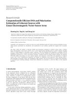
From the geometric perspective, a quad-quaternion p
=
p
0
+ip
1
+ jp
2
+kp
3
can be considered as a point in a 4D space
spanned by 1, i, j, k, as shown in Figure 1.Thedifference
from the quaternion case is that the 1, i, j, k coefficients of
Xiaofeng Gong et al. 3
Table 1: Symbols of algebraic values.
R
Real numbers
C
(L)
Complex numbers with bases {1, L},whereL = i, j, k,I, J, K.Inparticular,C
(i)

is denoted by C.
H
(a,b)
Quaternions with bases {1, i, j, k} such that i
2
= a, j
2
= b and ij =−ji = k,wherea and b are nonzero real numbers. In
particular,
H
=
H
(−1,−1)
corresponds to the classical Hamilton quaternions
H
(1)
, H
(2)
H
(1)
denotes Hamilton’s quaternions with bases {1,i, j, k}; H
(2)
denotes the Hamilton quaternions with bases {1,I, J, K}.
In particular, we denote
H
(1)
by H.
H
C
(L)

Biquaternions with bases {1, i, j, k, L, Li, Lj, Lk}, L = I, J, K, such that i
2
=−1, j
2
=−1, ij =−ji = k and lL = Ll,where
l
= i, j, k.Inparticular,wedenoteH
C
(I)
by H
C
.
H
H
Quad-quaternions with bases {1, i, j, k, I, Ii, Ij, Ik,J, Ji, Jj,Jk, K, Ki, Kj, Kk} such that i
2
= j
2
= I
2
= J
2
=−1,
ij
=−ji = k, IJ =−JI = K,andlL = Ll,wherel = i, j, k and L = I, J, K.
p are not real values, but four individual quaternions which
can be considered as four subpoints in a 4D hypospace
spanned by 1, I, J, K. Therefore, quite similar to quaternion
rotations [38], we can interpret quad-quaternion multiplica-
tions as a more complex 16D “quad-quaternion rotations”

which involve both 4D rotations(quaternion multiplica-
tions) and combination of 4D points (quaternion additions)
in spaces spanned by 1,i, j, k and 1, I, J, K.
Definition 2. A quad-quaternion matrix Q
∈ (H
H
)
M×N
is a
matrix with M rows and N columns of which each element
is a quad-quaternion q
m,n
∈ H
H
, m = 1, 2, , M, n =
1, 2, , N. In particular, an N dimensional quad-quaternion
column (row) vector can be considered as an N
× 1(1×
N) quad-quaternion matrix. In this paper, quad-quaternion
vectors are specifically referred to as column vectors. Similar
to the case of quad-quaternion scalars, a quad-quaternion
matrix Q
∈ (H
H
)
M×N
can be expressed as follows:
Q
=


Q
00
+ IQ
01
+ JQ
02
+ KQ
03

+ i

Q
10
+ IQ
11
+ JQ
12
+ KQ
13

+ j

Q
20
+ IQ
21
+ JQ
22
+ KQ
23


+ k

Q
30
+ IQ
31
+ JQ
32
+ KQ
33

=
Q
0
+ IQ
1
+ JQ
2
+ KQ
3
= B
0
+ IB
1
,
(4)
where Q
n
1

n
2
∈ R
M×N
, n
1
, n
2
= 0, 1,2, 3, Q
n
∈ H
M×N
,
n
= 0, 1, 2, 3, and B
0
, B
1
∈ (H
C
(J)
)
M×N
. Similar to quad-
quaternion scalars, the scalar and vector parts of Q are given
by S(Q)
= Q
00
and V(Q) = Q −S(Q), respectively.
In the following discussion, we mainly focus on results

related to quad-quaternion matrices and vectors. The results
related to scalars can be directly obtained by considering a
quad-quaternion scalar as a 1
×1 quad-quaternion “matrix.”
2.2. Previous relevant results
In this section, we present some results that are directly
generalized from quaternion or biquaternion results. All
the lemmas in this section can be proved similarly to their
quaternion and biquaternion counterparts in [35–37], and
thus are not included in this paper.
K
IJ
1
k
i
j
1
K
I
J
1
K
I
J
1
K
I
J
1
p

3
p
3
p
0
p
2
p
2
p
1
p
1
p = p
0
+ ip
1
+ jp
2
+ kp
3
Figure 1: The geometric illustration of quad-quaternions.
Definition 3 ([37, Definition 2]). There exist four different
conjugations for quad-quaternion matrices as follows.
(i)
C-conjugation Q
C
: Q
C
= B

0
−IB
1
;
(ii)
H
1
-conjugation Q

: Q

= Q
∗
0
+ IQ
∗
1
+ JQ
∗
2
+ KQ
∗
3
;
(iii)
H
2
-conjugation Q
∗
: Q

∗
= Q
0
−IQ
1
−JQ
2
−KQ
3
;
(iv) Total-conjugation
Q: Q = Q
∗
0
−IQ
∗
1
−JQ
∗
2
−KQ
∗
3
,
where Q
∗
n
denotes the quaternion conjugation of Q
n
, n =

0, 1, 2, 3, as given in [36].
Definition 4 (from [37]). The transpose of Q
= Q
0
+ IQ
1
+
JQ
2
+ KQ
3
∈ (H
H
)
M×N
,denotedbyQ
T
∈ (H
H
)
N×M
,is
defined as Q
T
 Q
T
0
+ IQ
T
1

+ JQ
T
2
+ KQ
T
3
,whereQ
T
n
denotes
the quaternion transpose of Q
n
, n = 0, 1, 2, 3. Then we have
the following four different conjugated transposes.
(i)
C-conjugated transpose Q

: Q

= (Q
C
)
T
= (Q
T
)
C
;
(ii)
H

1
-conjugated transpose Q
H
1
: Q
H
1
=(Q

)
T
=(Q
T
)

;
(iii)
H
2
-conjugated transpose Q
H
2
: Q
H
2
=(Q
∗
)
T
=(Q

T
)
∗
;
(iv) Total-conjugated transpose Q
H
: Q
H
= (Q)
T
= Q
T
.
Definition 5 ([37, Definition 3]). The norm of a quad-
quaternion p
= p
0
+ Ip
1
+ Jp
2
+ Kp
3
,denotedby|p|,is
given by
|p|=



p

0


2
+


p
1


2
+


p
2


2
+


p
3


2
. (5)
4 EURASIP Journal on Advances in Signal Processing

By definition, we can see that the following equation holds:
S(
pp) = S

p
∗
0
−Ip
∗
1
−Jp
∗
2
−Kp
∗
3

p
0
+Ip
1
+Jp
2
+Kp
3

=
S

p

∗
0
p
0
+ p
∗
1
p
1
+ p
∗
2
p
2
+ p
∗
3
p
3

+ I

p
∗
0
p
1
+ p
∗
3

p
2
− p
∗
1
p
0
− p
∗
2
p
3

+ J

p
∗
0
p
2
+ p
∗
1
p
3
− p
∗
2
p
0

− p
∗
3
p
1

+ K

p
∗
0
p
3
+ p
∗
2
p
1
− p
∗
3
p
0
− p
∗
1
p
2

=


p
∗
0
p
0
+ p
∗
1
p
1
+ p
∗
2
p
2
+ p
∗
3
p
3

=|
p|
2
.
(6)
It is important to note that
|pq|
/

=|p||q|, so that quad-
quaternions do not form a normed algebra. We can further
define the norm of a quad-quaternion vector q
∈ (H
H
)
N×1
by
q 

S

q
H
q

. (7)
Definition 6 (see (15) from [37]). Two quad-quaternion
vectors a, b
∈ (H
H
)
N×1
are said to be orthogonal if
a
H
b = 0. (8)
Definition 7 (see (17) from [37]). The adjoint matrix (χ
Q
∈

(H
C
(J)
)
2M×2N
) of a quad-quaternion matrix Q ∈ (H
H
)
M×N
=
B
0
+ IB
1
(where B
0
, B
1
∈ (H
C
(J)
)
M×N
)isgivenby
χ
Q


B
0

B
∗
1
−B
1
B
∗
0

. (9)
Let further Ψ
M
 [I
M
, −I · I
M
] ∈ (C
(I)
)
M×2M
,whereI
M
is the identity matrix of size M × M, then
Q
=
1
2
Ψ
M
χ

Q
Ψ
H
N
, (10)
where
Ψ
M
Ψ
H
M
= 2I
M
,
χ
Q
Ψ
H
N
Ψ
N
= Ψ
H
M
Ψ
M
χ
Q
.
(11)

Lemma 1 (from [35]). Consider two quad-quaternion matri-
ces A
∈ (H
H
)
M×N
and B ∈ (H
H
)
N×L
, and denote the adjoint
matrices of A, B,andAB by χ
A
, χ
B
,andχ
AB
,respectively,then
χ
AB
= χ
A
·χ
B
. (12)
Lemma 2 ([37, Lemma 1]). If P
H
= P, then P ∈ (H
H
)

N×N
is Hermitian. Then we note that the adjoint matrix of a
Hermitian quad-quaternion matrix is also Hermitian.
Definition 8 (from [37]). If Qu
= uλ,whereu ∈ (H
H
)
N×1
,
λ
∈ C,andQ ∈ (H
H
)
N×N
, then λ and u are, respectively, the
right eigenvalue and the associated right eigenvector of Q.
Lemma 3 ([37, Lemma 2]). Denote the adjoint matrix of Q
∈
(H
H
)
N×N
by χ
Q
,ifλ ∈ C and u
b
∈ (H
C
(J)
)

2N×1
are the right
eigenvalue and the associated right eigenvector of χ
Q
, then λ
and u
= Ψ
N
u
b
are the right eigenvalue and the associated right
eigenvector of Q.
Corollary 1 (from [37]). The eigenvalues of a Hermitian
quad-quaternion matrix are real values. Consider a Hermitian
quad-quaternion mat rix Q
∈ (H
H
)
N×N
whose adjoint mat rix
χ
Q
can be eigendecomposed as χ
Q
= U
b
DU
H
b
,whereU

b
∈
(H
C
)
2N×4N
,andD ∈ R
(4N×4N)
is a real diagonal matrix. The
eigendecomposition of Q is then given by
Q = UDU
H
=
4N

n=1
λ
n
u
n
u
H
n
, (13)
where U
= (1/
√
2)Ψ
N
U

b
∈ (H
H
)
N×4N
, λ
n
is the nth element
of the diagonal of D, u
n
is the nth column vector of U.
Lemma 4. The eigenvectors corresponding to different eigen-
values of a Hermitian quad-quaternion matrix are orthogonal.
2.3. New definitions and lemmas for
quad-quaternioins
In this section, we introduce some new results related to
quad-quaternions. For an easier reading of this section, all
the results are given directly, while some of their proofs are
summarized in the appendix for the reference of interested
readers.
Definition 9. Let Λ
={1, i, j, k, I, Ii,Ij, Ik, J, Ji,Jj, Jk, K, Ki,
Kj, Kk
} and Γ ⊆ Λ, then the Γ-match of a quad-quaternion
matrix Q
∈ (H
H
)
M×N
,denotedbyS(Q | Γ), is obtained

by keeping the coefficients of the units in Γ unchanged, and
setting all the other coefficients to zero. The Γ-complement
of Q is defined as V(Q
| Γ)  Q −S(Q | Γ).
By definition, we know that the match and complement
operations are used to select some desired parts of quad-
quaternions. For example, if Γ
={1, i, K}, then S(Q | Γ) =
Q
00
+iQ
10
+KQ
03
,whereQ
00
, Q
10
, Q
03
are given in (4). Also it
can be proved that V(Q
| Γ
⊥
) = S(Q | Γ), where Γ
⊥
denotes
the complement of Γ.Particularly,ifΓ
={1}, S(Q | Γ)and
V(Q

| Γ) are equal to the scalar part and the vector part of
Q,respectively.
Definition 10. Let Λ
={1, i, j, k, I, Ii, Ij, Ik,J, Ji, Jj,Jk,K, Ki,
Kj, Kk
},andΓ ⊆ Λ, then the Γ-conjugation of a quad-
quaternion matrix Q
= S(Q | Γ)+V(Q | Γ) ∈ (H
H
)
M×N
is denoted by conj(Q | Γ),anddefinedas
conj(Q
| Γ)  S(Q | Γ) − V(Q | Γ). (14)
It should be noted that the four conjugations given in
Definition 3 are actually four special examples of the Γ-
conjugation corresponding to different selections of Γ.
For example, the
H
1
-conjugation corresponds to Γ =
{
1, I, J, K}, whereas the total-conjugation corresponds to Γ =
{
i, j, k, I, J, K}
⊥
.
Lemma 5. Given two sets Γ
1
, Γ

2
⊆ Λ,wehave
conj

conj

Q | Γ
1

|
Γ
2

=
conj

Q |

Γ
1
∩Γ
2

∪

Γ
1
∪Γ
2


⊥

,
(15)
Xiaofeng Gong et al. 5
where Γ
1
∩Γ
2
and Γ
1
∪Γ
2
denote the intersection and union of
Γ
1
and Γ
2
,respectively.
Definition 11. Let Λ
={1, i, j, k, I, Ii, Ij, Ik,J, Ji, Jj,Jk,K, Ki,
Kj, Kk
} and Γ ⊆ Λ, the Γ-conjugated transpose of Q is
given by conj(Q
| Γ)
T
.Itiseasytoprovethatconj(Q | Γ)
T
=
conj(Q

T
| Γ). Also, when Γ = Λ, Q
T
= conj(Q | Γ)
T
.
Similar to the Γ -conjugation, the four different conjugated
transposes given in Definition 4 are four different examples
corresponding to four different selections of Γ.
Definition 12. Quad-quaternion vectors v
1
, v
2
, , v
N
∈
(H
H
)
M×1
are said to be right (left) linear dependent if there
are scalars μ
1
, μ
2
, , μ
N
∈ H
H
not all zero, such that v

1
μ
1
+
v
2
μ
2
+ ···+ v
N
μ
N
= o
M×1
(μ
1
v
1
+ μ
2
v
2
+ ···+ μ
N
v
N
=
o
M×1
). Moreover, if v

1
μ
1
+ v
2
μ
2
+ ··· + v
N
μ
N
= o
M×1
(μ
1
v
1
+ μ
2
v
2
+ ···+ μ
N
v
N
= o
M×1
)istrueifandonly
if μ
1

, μ
2
, , μ
N
are all zero, vectors v
1
, v
2
, , v
N
are said
to be right (left) linearly independent. Here, o
N×1
is an
N
× 1 zero vector. Obviously, since v
1
μ
1
/
=μ
1
v
1
in most
cases, the concept of right linear dependent (independent)
is different from that of left linear dependent (indepen-
dent).
Definition 13. Given a set of quad-quaternion vectors
v

1
, v
2
, , v
N
∈ (H
H
)
M×1
,ifv
1
, v
2
, , v
R
(R<N),
are right (left) linearly independent and there exists an
arbitrary vector v
R+1
∈ (H
H
)
M×1
such that v
1
, v
2
, , v
R+1
are right (left) linearly dependent, then v

1
, v
2
, , v
R
form
a maximal right (left) linearly independent set. Further-
more, we define the right (left) rank of
{v
1
, v
2
, , v
N
}
as rank
R
({v
1
, v
2
, , v
R
})  R (rank
L
({v
1
, v
2
, , v

R
}) 
R).
Definition 14. Given a quad-quaternion matrix P
= [p
1
,
p
2
, , p
N
], where p
n
is the nth column of P, n =
1, 2, , N. Then the right (left) rank of P is defined
as rank
R
(P)  rank
R
({p
1
, p
2
, , p
N
})(rank
L
(P) 
rank
L

({p
1
, p
2
, , p
N
})). In addition, we have the following
lemma.
Lemma 6. Denote the adjoint matrix of P
∈ (H
H
)
N×N
by χ
P
,
then
rank
R
(P) =
1
2
rank
R

χ
P


rank

L
(P) =
1
2
rank
L

χ
P


.
(16)
In the follow ing discussion, we only consider the r ight rank, and
we denote rank(P)
= rank
R
(P).
Lemma 7. Denote the eigenvalue decomposition of a Hermi-
tian quad-quaternion matri x Q by Q
= UDU
H
, then we have
rank(Q)
=
1
4
rank(D). (17)
Definition 15. Given a set of orthogonal quad-quaternion
vectors v

1
, v
2
, , v
N
, we can define the vector space R
spanned by v
1
, v
2
, , v
N
as R 

v | v = v
1
μ
1
+
v
2
μ
2
+ ··· + v
N
μ
N

,whereμ
1

, μ
2
, , μ
N
are arbitrary
quad-quaternion scalars. R can also be denoted as R
=
span(v
1
, v
2
, , v
N
).
Lemma 8. If v
1
, v
2
, , v
N
are N eigenvectors of a Her mitian
quad-quaternion matrix, then v
1
μ
1
, v
2
μ
2
, , v

N
μ
N
are also
a set of eigenvectors of this Hermitian quad-quaternion
matrix, where μ
1
, μ
2
, , μ
N
are nonzero quad-quaternions.
Then, we have span(v
1
, v
2
, , v
N
) = span(v
1
μ
1
, v
2
μ
2
, ,
v
N
μ

N
).
This lemma indicates that the indetermination of eigen-
vectors of a Hermit ian quad-quaternion matrix does not
impact their span. From the geometric perspective, when
the eigenvector multiplies a nonzero scalar from the right
side, all the elements of this eigenvector are rotated in the
16D quad-quaternion space (as shown in Figure 1)with
the same quad-quaternion manner, and the proportional
relationship between different elements does not change.
Therefore, the intrinsic “structure” of this eigenvector is
independent of the above-mentioned eigenvector indetermi-
nation.
3. QUAD-QUATERNION MUSIC
3.1. Quad-quaternion model for EM vector sensors
Let (θ, ϕ)and(γ, η) be the azimuth-elevation 2D DOA (see
Figure 2) and polarization of an EM signal, respectively,
where 0 <θ
≤ 2π,0≤ ϕ ≤ π,and0≤ γ ≤ π/2, −π ≤ η ≤ π.
The output of an EM vector sensor then can be capsulated
into the following quad-quaternion scalar:
p
(θ,ϕ,γ,η)
= i

E
(θ,ϕ,γ,η)
x
+ IH
(θ,ϕ,γ,η)

x

+ j

E
(θ,ϕ,γ,η)
y
+ IH
(θ,ϕ,γ,η)
y

+ k

E
(θ,ϕ,γ,η)
z
+ IH
(θ,ϕ,γ,η)
z

,
(18)
where E
(θ,ϕ,γ,η)
x
, E
(θ,ϕ,γ,η)
y
, E
(θ,ϕ,γ,η)

z
∈ C
(J)
,andH
(θ,ϕ,γ,η)
x
,
H
(θ,ϕ,γ,η)
y
, H
(θ,ϕ,γ,η)
z
∈ C
(J)
are the three components of the
electric vector and the magnetic vector, respectively, which
are defined as [2]
⎛
⎜
⎜
⎜
⎜
⎜
⎜
⎜
⎜
⎜
⎜
⎜

⎜
⎜
⎜
⎜
⎝
E
(θ,ϕ,γ,η)
x
E
(θ,ϕ,γ,η)
y
E
(θ,ϕ,γ,η)
z
H
(θ,ϕ,γ,η)
x
H
(θ,ϕ,γ,η)
y
H
(θ,ϕ,γ,η)
z
⎞
⎟
⎟
⎟
⎟
⎟
⎟

⎟
⎟
⎟
⎟
⎟
⎟
⎟
⎟
⎟
⎠

⎛
⎜
⎜
⎜
⎜
⎜
⎜
⎜
⎜
⎜
⎜
⎝
−
sin θ cos ϕ cos θ
cos θ cos ϕ sin θ
0
−sin ϕ
−cos ϕ cos θ −sin θ
−cos ϕ sinθ cos θ

sin ϕ 0
⎞
⎟
⎟
⎟
⎟
⎟
⎟
⎟
⎟
⎟
⎟
⎠
·

cos γ
sin γe
Jη


 
h
γ,η
∈

C
(J)

2×1
.

(19)
Thus, (18)canberewrittenas
6 EURASIP Journal on Advances in Signal Processing
p
θ,ϕ,γ,η
=
⎧
⎪
⎪
⎪
⎪
⎪
⎪
⎪
⎪
⎨
⎪
⎪
⎪
⎪
⎪
⎪
⎪
⎪
⎩
Θ
(1)
θ,ϕ
∈


C
(I)

1×2
  

−
sin θ −I ·cos ϕcos θ
cos ϕ cos θ
−I ·sinθ

T
·i+
Θ
(2)
θ,ϕ
∈

C
(I)

1×2
  

cos θ −I ·cos ϕ sin θ
cos ϕ sin ϕ + I
·cos ϕ

T
·j+

Θ
(3)
θ,ϕ
∈

C
(I)

1×2
  
I · sin ϕ
−sin ϕ
T
·k
  
Θ
θ,ϕ
∈H
1×2
C
⎫
⎪
⎪
⎪
⎪
⎪
⎪
⎪
⎪
⎬

⎪
⎪
⎪
⎪
⎪
⎪
⎪
⎪
⎭
·
h
γ,η
.
(20)
For an array of N EM vector sensors, the spatial steering
vector d
θ,ϕ
is given by
d
θ,ϕ
=

e
J·2π(k
T
1
e
θ,ϕ
/λ)
, , e

J·2π(k
T
N
e
θ,ϕ
/λ)

T
, (21)
where k
n
is the position vector of the nth EM vector sensor,
e
θ,ϕ
is the propagation vector corresponding to (θ, ϕ), λ is the
wavelength of incident signals. The steering vector of such an
N-element EM vector-sensor array then can be expressed as
a
θ,ϕ,γ,η
= p
θ,ϕ,γ,η
d
θ,ϕ
=

Θ
θ,ϕ
⊗d
θ,ϕ


h
γ,η
=

Θ
(1)
θ,ϕ
⊗d
θ,ϕ

h
γ,η
  
a
(1)
θ,ϕ,γ,η
·i +

Θ
(2)
θ,ϕ
⊗d
θ,ϕ

h
γ,η
  
a
(2)
θ,ϕ,γ,η

· j
+

Θ
(3)
θ,ϕ
⊗d
θ,ϕ

h
γ,η
  
a
(3)
θ,ϕ,γ,η
·k,
(22)
where “
⊗”denotestheKroneckerproduct.
In the presence of M narrowband, far-field, and com-
pletely polarized signals, the quad-quaternion model of an
N-element EM vector-sensor array has the following form:
x(t)
=
M

m=1
a
m
s

m
(t)+n(t)
=
M

m=1

Θ
m
⊗d
m

·
h
m

·
s
m
(t)+n(t),
(23)
where s
m
(t) ∈ C
(J)
is the complex envelop of the mth signal,
and n(t) is the additive noise term, and d
m
= d
θ

m
,ϕ
m
, p
m
=
p
θ
m
,ϕ
m
,γ
m
,η
m
, Θ
m
= Θ
θ
m
,ϕ
m
, h
m
= h
γ
m
,η
m
. It is assumed here

that (1) all the incident signals are uncorrelated; (2) the
noise is spatially white and uncorrelated with the signals;
(3) steering vectors corresponding to different selections of
(θ, ϕ, γ, η) are right linearly independent.
3.2. Algorithm details
We first define the quad-quaternion array manifold Φ as the
continuum of steering vector a
θ,ϕ,γ,η
in the angular parameter
space of interest I
1
and the polarization parameter space of
interest I
2
. That is,
Φ 

a
θ,ϕ,γ,η
,(θ,ϕ) ∈ I
1
,(γ, η) ∈ I
2

. (24)
Moreover, the signal subspace and noise subspace in quad-
quaternion case are defined as follows:
R
s
= span


a
1
, , a
M

,
R
n
= R
⊥
s
.
(25)
Define the covariance matrix with quad-quaternion entries
as
R
x
= E

x

t
l

x
H

t
l


, (26)
where “E” denotes expectation. From (23),
R
x
=
M

m=1
σ
2
m
a
m
a
H
m
+ R
n
, (27)
where σ
2
m
= E[s
m
(t)s
∗
m
(t)] and R
n

= E[n(t)n
H
(t)] = σ
2
n
I
N
.
It can be easily proven according to Definition 14 that
the rank of A
= [a
1
, a
2
, , a
M
]isM, then in the absence
of noise, the rank of R
x
= diag([σ
2
1
, σ
2
2
, , σ
2
M
])AA
H

is M,
and the column vectors of R
x
span the signal subspace R
s
.In
the presence of noise, we apply an M-rank approximation
of R
x
to estimate the bases of signal subspace. According
to Lemma 7, we know that the best M-rank approximation
of R
x
has 4M eigenvalues, thus we can use the eigenvectors
v
1
, , v
4M
associated with the largest 4M eigenvaluesasthe
bases of signal subspaces. Denote E
s
= [v
1
, , v
4M
]andE
n
=
[v
4M

, , v
4N
], then R
s
= span(E
s
)andR
n
= span(E
n
).
Further, define P
n
= E
n
E
H
n
∈ H
N×N
H
,wehaveP
n
a
m
=0,
then

θ
m

, ϕ
m

= arg

min
θ,ϕ,γ,η


P
n
a
θ,ϕ,γ,η



. (28)
In the presence of finite data length, R
x
can be estimated
as follows:

R
x
=
1
L
L

l=1

x(t
l
)x
H
(t
l
). (29)
Accordingly, E
n
and P
n
can be estimated by eigendecompos-
ing

R
x
.
A question of fundamental interests is whether the
indetermination of quad-quaternion eigenvectors impacts
the results of MUSIC. According to Lemma 8, the indeter-
mination of eigenvectors does not impact the vector space
spanned by them, and thus does not impact the estimation
of noise subspace. Since the performance of MUSIC-like
algorithms is mainly dependent on the accuracy of subspace
estimation, the indetermination of eigenvectors does not
impact the results of quad-quaternion MUSIC.
Xiaofeng Gong et al. 7
3.3. Decoupling of angular and polarization
parameters
According to (28),a4DsearchisrequiredforDOA

estimation, which might be computationally prohibitive.
We next discuss how to decouple polarization from DOA
estimation for the purpose of reducing the computational
burden. Firstly, we prove the following lemma.
Lemma 9. Given h
∈ (C
(L)
)
M×1
, L ∈{i, j, k, I, J,K} and a
Hermitian matrix F
∈ (H
H
)
M×M
, then S(h
H
Fh) = h
H
S(F |
{
1, L})h.Here,S(h
H
Fh) and S(F |{1,L}) denote the scalar
part of h
H
Fh and the {1, L}-match of F,respectively.
Proof. Without loss of generality, we assume L
= J.Hence,
h

∈ (C
(J)
)
M×1
. Let further F = (F
00
+ IF
01
)+i(F
10
+ IF
11
)+
j(F
20
+ F
21
)+k(F
30
+ F
31
), then S(F |{1, J}) = F
00
. Since
F
H
= F,wehaveF
H
00
= F

00
. Then it is further obtained that
S

h
H
Fh

=
S

h
H

F
00
+ IF
01

+ i

F
10
+ IF
11

+ j

F
20

+ F
21

+ k

F
30
+ F
31

h

=
S

h
H
F
00
h

=
h
H
F
00
h = h
H
S


F |{1, J}

h.
(30)
We use the above-mentioned lemma to discuss the
decoupling of angular and polarization parameters. Let u
=
P
n
a
θ,ϕ,γ,η
∈ H
(N×1)
H
, then


P
n
a
θ,ϕ,γ,η


=

S

u
H
u


. (31)
According to (23), and denote Ξ
θ,ϕ
= P
n
· Θ
θ,ϕ
⊗ d
θ,ϕ
, then
we have the following equation from Lemma 9:
S

u
H
u

= S

h
H
γ,η
Ξ
H
θ,ϕ
Ξ
θ,ϕ
h
γ,η


= h
H
γ,η
S

Ξ
H
θ,ϕ
Ξ
θ,ϕ
|{1, J}

h
γ,η
.
(32)
Note further that h
H
γ,η
h
γ,η
= 1andS(Ξ
H
θ,ϕ
Ξ
θ,ϕ
|{1, J})is
a complex-valued Hermitian matrix, then according to the
Rayleigh-Ritz theorem [11], we obtain

min
θ,ϕ,γ,η


P
n
a
θ,ϕ,γ,η


=
min
θ,ϕ,γ,η

h
H
γ,η
S

Ξ
H
θ,ϕ
Ξ
θ,ϕ
|{1, J}

h
γ,η
h
H

γ,η
h
γ,η

=
λ
min

S

Ξ
H
θ,ϕ
Ξ
θ,ϕ
|{1, J}

,
(33)
where λ
min
(S(Ξ
H
θ,ϕ
Ξ
θ,ϕ
|{1, J})) denotes the smallest eigen-
value of S(Ξ
H
θ,ϕ

Ξ
θ,ϕ
|{1, J}). Thus, the 4D search problem is
reduced to a 2D search.
For clarity, we finally summarize the above split method
(termed as QQ-MUSIC) as follows:
Step 1. calculate the sampled covariance matrix

R
x
according
to (29);
Step 2. apply the quad-quaternion EVD to

R
x
, select the
4(N
− M) eigenvectors associated to the smallest 4(N − M)
eigenvalues, and calculate the noise subspace projector P
n
;
z
y
x
θ
ϕ
Figure 2: Coordinate system and angle definition.
Step 3. givenanarbitrary(θ, ϕ) ∈ I
1

,calculateΞ
θ,ϕ
= P
n
·
Θ
θ,ϕ
⊗d
θ,ϕ
and S(Ξ
H
θ,ϕ
Ξ
θ,ϕ
|{1, J}).
Step 4. then the DOA estimates are obtained by
arg min
(θ,ϕ)∈I
1

λ
min

F
θ,ϕ

. (34)
It is important to note that QQ-MUSIC cannot ful-
fill simultaneous estimation of DOA and polarization.
The problem of polarization estimation or joint DOA-

polarization estimation remains unresolved and is currently
under investigation by the authors.
3.4. Computation complexity
In this section, the computational complexity of QQ-
MUSIC, BQ-MUSIC, and long-vector MUSIC is addressed.
As addressed in [36, 37], the covariance matrix estimation
best illustrates the complexity difference of the three algo-
rithms, therefore we only consider the computational com-
plexity involved in this part. The evaluation of computational
complexity includes two aspects: memory requirement and
number of real number additions (A), multiplications (M),
and divisions (D).
Assume that the array comprises N complete EM vector
sensors, and T snapshot vectors are available. The quad-
quaternion array output X
∈ (H
H
)
N×T
then is given by
X
= X
0
+IX
1
=

iX
01
+ jX

02
+kX
03

+I

iX
11
+ jX
12
+kX
13

,
(35)
where X
0
, X
1
∈ (H
C
(J)
)
N×T
,andX
0n
, X
1n
∈ (C
(J)

)
N×T
,
n
= 1, 2, 3. Then the biquaternion data model (X
b
∈
(H
C
(J)
)
2N×T
) and the long-vector data model (X
lv
∈
(C
(J)
)
6N×T
) for the same array output are, respectively,
written as
X
b
=

X
T
0
, X
T

1

T
, X
lv
=

X
T
01
, X
T
02
, X
T
03
, X
T
11
, X
T
12
, X
T
13

T
.
(36)
Moreover, the sampled covariance matrices in the three

models can be calculated as follows:

R
Q
=
1
T
XX
H
,

R
B
=
1
T
X
b
X
H
b
,

R
LV
=
1
T
X
lv

X
H
lv
,
(37)
8 EURASIP Journal on Advances in Signal Processing
Table 2: Computational effort for covariance estimation.
Memory requirements (complex values) Real multiplications Real additions Real divisions
QQ-MUSIC 8N
2
256N
2
T (256T − 16)N
2
16N
2
(D)
BQ-MUSIC 16N
2
256N
2
T (256T − 32)N
2
32N
2
(D)
LV-MU SI C 36 N
2
144N
2

T (144T − 72)N
2
72N
2
(D)
where

R
Q
,

R
B
,

R
LV
are sampled covariance matrices used in
QQ-MUSIC, BQ-MUSIC, and LV-MUSIC, respectively.
From (37),

R
Q
has N
2
entries, each of which is quad-
quaternion valued and can be represented by eight complex
numbers. Therefore, a memory of at least 8N
2
complex

numbers is required in the quad-quaternion case. Similarly,
for biquaternion and long-vector models, 16N
2
and 36N
2
complex numbers are required, respectively.
Let us now evaluate the total number of basic arithmetic
operations needed for estimation of the covariance matrix.
As revealed by (37), every entry of

R
Q
is obtained by T
quad-quaternion multiplications, T
− 1 quad-quaternion
additions, and a division by a real value. Note that one quad-
quaternion multiplication implies 16
2
real multiplications
plus 16
× 15 real additions, one quad-quaternion addition
implies 16 real additions, and the division by a real value
equals 16 real divisions. The number of operations needed
for one entry is

16
2
(M)
+16×15
(A)


T + 16(T − 1)
(A)
+16
(D)
,
where subscripts “(M),” “(A),” “(D)” denote real multiplica-
tion, real addition, and real division, respectively. Thus, the
total number is
{[16
2
(M)
+16×15
(A)
]T+16(T − 1)
(A)
+16
(D)
}·
N
2
= 256N
2
T
(M)
+ (256T − 16)N
2
(A)
+16N
2

(D)
. Similarly,
the total numbers of arithmetic operations in biquaternion
and long-vector models are given by 256N
2
T
(M)
+ (256T −
32)N
2
(A)
+32N
2
(D)
and 144N
2
T
(M)
+ (144T − 72)N
2
(A)
+
72N
2
(D)
,respectively.Tab l e 2 summarizes the covariance
matrix computational efforts for all the three algorithms.
We can see that QQ-MUSIC largely reduces the memory
requirements, mainly due to the more economical formulism
of quad-quaternion model. In addition, with regard to

basic arithmetic operation number, we can see that QQ-
MUSIC requires 16N
2
less real divisions and 16N
2
more
real additions than BQ-MUSIC. Since the computational
complexity of divisions is much more than that of additions,
QQ-MUSIC slightly outperforms BQ-MUSIC in this aspect.
We may also note that LV-MUSIC requires least operations
for estimating the covariance matrix, which conflicts our
intuition that a more concise model should lead to less
computational complexity. This fact can be explained as
follows. In QQ-MUSIC, we are using a 16D algebra to model
six-component vector sensors, and only twelve imaginary
units of quad-quaternions are used in this formulation.
Therefore, this insufficient use of quad-quaternions results
in more arithmetic operations.
3.5. Orthogonality-measure comparison
As addressed in [37], vector orthogonality in higher dimen-
sional algebra imposes stronger constraints on vector com-
ponents. In this part, we take a further look into the quad-
quaternion-related orthogonality.
Consider two quad-quaternion vectors x, y
∈ (H
H
)
N
x
×1

given by
x
=

x
01
+ Ix
11

i +

x
02
+ Ix
12

j +

x
03
+ Ix
13

k,
y
=

y
01
+ Iy

11

i +

y
02
+ Iy
12

j +

y
03
+ Iy
13

k.
(38)
The corresponding biquaternion representation and com-
plex representation then can be written as
x
bq
=

x
T
01
, x
T
11


T
i +

x
T
02
, x
T
12

T
j +

x
T
03
, x
T
13

T
,
k ∈

H
C

2N
x

×1
,
y
bq
=

y
T
01
, y
T
11

T
i +

y
T
02
, y
T
12

T
j +

y
T
03
, y

T
13

T
,
k ∈

H
C

2N
x
×1
,
x
c
=

x
T
01
, x
T
11
, x
T
02
, x
T
12

, x
T
03
, x
T
13

T
∈

C
(J)

6N
x
×1
,
y
c
=

y
T
01
, y
T
11
, y
T
02

, y
T
12
, y
T
03
, y
T
13

T
∈

C
(J)

6N
x
×1
.
(39)
Imposing the orthogonal constraint on quad-quaternion
vectors (x
H
y = 0) yields
x
H
01
y
01

+ x
H
11
y
11
+ x
H
02
y
02
+ x
H
12
y
12
+ x
H
03
y
03
+ x
H
13
y
13
= 0,
x
T
01
y

11
−x
T
11
y
01
+ x
T
02
y
12
−x
T
12
y
02
+ x
T
03
y
13
−x
T
13
y
03
= 0,
x
H
02

y
03
+ x
H
12
y
13
−x
H
03
y
02
−x
H
13
y
12
= 0,
x
T
02
y
13
−x
T
12
y
03
−x
T

03
y
12
+ x
T
13
y
02
= 0,
x
H
03
y
01
+ x
H
13
y
11
−x
H
01
y
03
−x
H
11
y
13
= 0,

x
T
03
y
11
−x
T
13
y
01
−x
T
01
y
13
+ x
T
11
y
03
= 0,
x
H
01
y
02
+ x
H
11
y

12
−x
H
02
y
01
−x
H
12
y
11
= 0,
x
T
01
y
12
−x
T
11
y
02
−x
T
02
y
11
+ x
T
12

y
01
= 0.
(40)
In contrast, orthogonal constraint on biquaternion vectors
(x
H
bq
y
bq
= 0) results in
x
H
01
y
01
+ x
H
11
y
11
+ x
H
02
y
02
+ x
H
12
y

12
+ x
H
03
y
03
+ x
H
13
y
13
= 0,
x
H
02
y
03
+ x
H
12
y
13
−x
H
03
y
02
−x
H
13

y
12
= 0,
x
H
03
y
01
+ x
H
13
y
11
−x
H
01
y
03
−x
H
11
y
13
= 0,
x
H
01
y
02
+ x

H
11
y
12
−x
H
02
y
01
−x
H
12
y
11
= 0.
(41)
Moreover, the orthogonal constraint on complex vectors
(x
H
c
y
c
= 0) leads to
x
H
01
y
01
+ x
H

11
y
11
+ x
H
02
y
02
+ x
H
12
y
12
+ x
H
03
y
03
+ x
H
13
y
13
= 0.
(42)
Xiaofeng Gong et al. 9
y
x
d
d

d
×

P
e
d ×

P
e
Actual sensor position
Ideal sensor position
Figure 3: An array with sensor position errors.
By comparing (40), (41)and(42), it is obtained that:
x
H
y = 0 =⇒ x
H
bq
y
bq
= 0 =⇒ x
H
c
y
c
= 0. (43)
Consequently, the quad-quaternion orthogonality can
impose stronger constraints than both biquaternion and
complex algebra do. This property of quad-quaternions
results in a better robustness of QQ-MUSIC to model errors,

as to be demonstrated in Section 4.
4. SIMULATION RESULTS
In this section, simulation results are provided to compare
the proposed QQ-MUSIC with both biquaternion-based
(such as BQ-MUSIC) and complex-based methods (such
as LV-MUSIC) for six-component EM vector-sensor arrays.
It should be noted that BQ-MUSIC was actually proposed
for three-component vector-sensor arrays [37]. Therefore,
we here use a 2
× 1 biquaternion vector to represent a
six-component vector sensor, and further we concatenate
these vectors into a biquaternion long-vector to enable BQ-
MUSIC.
We compare the proposed QQ-MUSIC with BQ-MUSIC,
LV-MUSIC, and polarimetric smoothing algorithm (PSA-
MUSIC [30]),intermsofrobustnesstomodelerrors
and DOA estimation performance under different levels of
signal-to-noise ratio (SNR). All the statistics shown here are
computed by averaging the results of 200 independent trials.
The array used here is an L-shaped array that comprises
four and five EM vector sensors along the x-axis and y -axis,
respectively (see Figure 3). The spacing between two adjacent
EM vector sensors is d
= λ/2. Before representing the results,
we introduce the following two model errors.
y
x
z
b
a

(a)
y
x
z
b
a
Norm of the loop
(b)
Figure 4: A short dipole or loop with arbitrary orientation.
Sensor-position error
the positions of EM vector sensors are not precisely known.
In the simulations, we model such sensor position error by
additive uniformly distributed noise, that is,
k
n
= k
n
+

P
e
·d ·

ε
x
, ε
y
,0

T

, (44)
where
k
n
and k
n
are the actual and ideal position coordinates
of the nth EM vector sensor, respectively, ε
x
and ε
y
are
uniformly distributed noise terms, and P
e
is the power of
sensor position error.
Sensor-orientation error
the orientation angles of a dipole and a loop are illustrated
in Figure 4.Withanorientationangle(α, β), where α
∈
[0, 2π), β ∈ [0, π/2], the outputs of a dipole and a loop are,
respectively, given by
E
(θ,ϕ,γ,η)
α,β
= [cos α sinβ,sinα sin β,cosβ]
·

E
(θ,ϕ,γ,η)

x
, E
(θ,ϕ,γ,η)
y
, E
(θ,ϕ,γ,η)
z

T,
H
(θ,ϕ,γ,η)
α,β
= [cos α sinβ,sinα sin β,cosβ]
·

H
(θ,ϕ,γ,η)
x
, H
(θ,ϕ,γ,η)
y
, H
(θ,ϕ,γ,η)
z

T,
(45)
where E
(θ,ϕ,γ,η)
x

, E
(θ,ϕ,γ,η)
y
, E
(θ,ϕ,γ,η)
z
,andH
(θ,ϕ,γ,η)
x
, H
(θ,ϕ,γ,η)
y
,
H
(θ,ϕ,γ,η)
z
are given in (23). Let the orientation angles of
10 EURASIP Journal on Advances in Signal Processing
the three dipoles of the nth EM vector sensor be (α
1,n
, β
1,n
),
(
α
2,n
, β
2,n
), and (α
3,n

, β
3,n
), while the orientation angles of the
three loops be (
α
4,n
, β
4,n
), (α
5,n
, β
5,n
), and (α
6,n
, β
6,n
), then we
have

α
l,n
, β
l,n

=

α
l
, β
l


+

P
e

ε
α,l,n
, ε
β,l,n

,
l
= 1, ,6; n = 1, ,N,
(46)
where P
e
is the power of the sensor orientation error,
ε
α,l,n
, ε
β,l,n
are uniformly distributed noise terms, (α
1
, β
1
) =
(α
4
, β

4
) = (0, π/2), (α
2
, β
2
) = (α
5
, β
5
) = (π/2,π/2),
(α
3
, β
3
) = (α
6
, β
6
) = (0, 0) are the corresponding nominal
orientation angles in the absence of sensor orientation error.
Combining (22), (23), (45), and (46), the output of the nth
EM vector sensor equals
p
(n)
θ,ϕ,γ,η
=

⎛
⎝
cos ε

β,1,n
sin

ε
α,1,n
−ϕ

−
I ·

sin ε
β,4,n
sin θ −cos

ε
α,4,n
−ϕ

cos ε
β,4,n
cos θ

cos ε
β,1,n
cos θ cos

ε
α,1,n
−ϕ


+sinε
β,1,n
sin θ + I · cos ε
β,4,n
sin

ε
α,4,n
−ϕ

⎞
⎠
T
·i
+
⎛
⎝
cos ε
β,2,n
cos

ε
α,2,n
−ϕ

−I ·

sin ε
β,5,n
sin θ −sin


ε
α,5,n
−ϕ

cos ε
β,5,n
cos θ

cos ε
β,2,n
cos θ sin

ϕ − ε
1,2,n

+sinε
β,2,n
sin θ + I · cos ε
β,5,n
cos

ε
α,5,n
−ϕ

⎞
⎠
T
· j

+
⎛
⎝
sin ε
β,3,n
sin

ε
α,3,n
−ϕ

+ I ·

cos ε
β,6,n
sin θ −cos

ε
α,6,n
−ϕ

sin ε
β,6,n
cos θ

sin ε
β,3,n
cos θ cos

ε

α,3,n
−ϕ

−
cos ε
β,3,n
sin θ + I · sin ε
β,6,n
sin

ε
α,6,n
−ϕ

⎞
⎠
T
·k

·
h
γ,η
.
(47)
Accordingly, the quad-quaternion expressions of the steering
vector and the array output can be, respectively, modified as
a
θ,ϕ,γ,η
=


p
(1)
θ,ϕ,γ,η
e
J·2π(k
T
1
e
θ,ϕ
/λ)
, , p
(N)
θ,ϕ,γ,η
e
J·2π(k
T
N
e
θ,ϕ
/λ)

T,
x(t) =
M

m=1
a
θ
m
,ϕ

m
,γ
m
,η
m
s
m
(t)+n(t).
(48)
In the first experiment, we assume that only the sensor
position error exists. Three uncorrelated signals are from
(θ
1
, ϕ
1
) = (8
◦
,90
◦
), (θ
2
, ϕ
2
) = (35
◦
,90
◦
), and (θ
3
, ϕ

3
) =
(60
◦
,90
◦
) (to exclude the effect of DOA ambiguity on the
comparison, we here only consider azimuth angle estima-
tion), respectively, with polarizations (γ
1
, η
1
) = (45
◦
,0
◦
),
(γ
2
, η
2
) = (45
◦
,90
◦
), and (γ
3
, η
3
) = (45

◦
, 180
◦
), respectively.
The sensor noise is assumed to be Gaussian white and
uncorrelated with the incident signals. The overall root mean
square error (RMSE) performance measure used here is
defined as follows:
ε
=
1
M
M

m=1





1
N
N
s

n=1

θ
m
−


θ
n,m

2

, (49)
where

θ
n,m
is the estimate of true azimuth angle θ
m
in the
nth trial. It is plotted in Figure 5 that the curves of overall
RMSE against sensor position error power for QQ-MUSIC,
BQ-MUSIC, LV-MUSIC, and PSA-MUSIC wherein the SNR
and the number of snapshots are fixed as 30 dB and 1000,
respectively. It can be seen that QQ-MUSIC provides the best
estimation accuracy in the presence of sensor position error.
In the second experiment, we assume that only the sensor
orientation error exists. The DOAs and polarizations of the
incident signals are the same as the first example. The overall
RMSE curves of QQ-MUSIC, BQ-MUSIC, LV-MUSIC, and
Overall RMSE (degree)
0
0.2
0.4
0.6
0.8

1
1.2
1.4
Power of sensor-position error
00.01 0.02 0.03 0.04 0.05 0.06 0.07
QQ-MUSIC
BQ-MUSIC
LV-MUSIC
PSA-MUSIC
Figure 5: RMS estimation errors versus sensor position error
power.
PSA-MUSIC against the power of sensor orientation error
are plotted in Figure 6, wherein the SNR is constantly 30 dB.
We can see that QQ-MUSIC shows better robustness to
sensor orientation error than BQ-MUSIC and LV-MUSIC.
In particular, when the power of sensor orientation error is
high, QQ-MUSIC can still provide reliable DOA estimates. It
can also be observed that the performance of PSA-MUSIC
is independent of the senor orientation error. This can be
explained by noting that PSA-MUSIC does not preserve the
polarization information, and thus is independent of the
model error in the polarization dimension.
Xiaofeng Gong et al. 11
Overall RMSE (degree)
0
1
2
3
4
5

6
7
Power of sensor-orientation error
012345678910
QQ-MUSIC
BQ-MUSIC
LV-MUSIC
PSA-MUSIC
Figure 6: RMS estimation errors versus the power of sensor
orientation error.
Overall RMSE (degree)
0
0.2
0.4
0.6
0.8
1
1.2
SNR (dB)
−10 −8 −6 −4 −20 2 4 6 810
QQ-MUSIC
BQ-MUSIC
LV-MUSIC
PSA-MUSIC
Figure 7: RMS estimation errors versus SNR for an ideal EM
vector-sensor array.
We next compare the performance of QQ-MUSIC with
BQ-MUSIC, LV-MUSIC, and PSA-MUSIC with respect to
SNR. The DOAs and polarizations are the same as the first
two examples. The SNR is varied between

−10 dB and 10 dB.
Three cases are considered (1) in the absence of model error;
(2) in the presence of sensor position error only, and the
error power is P
e
= 0.05; (3) in the presence of sensor
orientation error only, with model error power P
e
= 5.
TheresultsaregiveninFigures7–9.FromFigure 7,ina
model error-free case, QQ-MUSIC and BQ-MUSIC are a
bit inferior to LV-MUSIC and PSA-MUSIC. From Figure 8,
we can see that QQ-MUSIC outperforms BQ-MUSIC, LV-
Overall RMSE (degree)
0.5
1
1.5
2
2.5
3
3.5
4
4.5
5
SNR (dB)
−10 −8 −6 −4 −20 2 4 6 810
QQ-MUSIC
BQ-MUSIC
LV-MUSIC
PSA-MUSIC

Figure 8: RMS estimation errors versus SNR in the presence of
sensor position errors.
Overall RMSE (degree)
0
2
4
6
8
10
12
14
SNR (dB)
−10 −8 −6 −4 −20 2 4 6 810
QQ-MUSIC
BQ-MUSIC
LV-MUSIC
PSA-MUSIC
Figure 9: RMS estimation errors versus SNR in the presence of
sensor orientation errors.
MUSIC, and PSA-MUSIC at all levels of SNR, in the
presence of sensor position errors; from Figure 9, we see that
QQ-MUSIC outperforms LV-MUSIC and PSA-MUSIC in
sensor orientation errors, while slightly underperforms PSA-
MUSIC because the performance of the latter is independent
of sensor orientation errors.
Then, we consider the case of several incident signals with
close DOAs and polarizations. An “L”-shaped array with 20
complete EM vector sensors is used, and six incident signals
are assumed to be impinging, among which the first and
the second signals, the third and the fourth signals, and the

fifth and the sixth signals are close to each other in both
12 EURASIP Journal on Advances in Signal Processing
QQ-MUSIC (dB)
10
−4
10
−3
10
−2
10
−1
10
0
Azimuth angle (degree)
10 20 30 40 50 60 70
Figure 10: QQ-MUSIC spectrum in the presence of several close
signals; SNR
=30 dB, the number of snapshots is 100.
BQ-MUSIC (dB)
10
−4
10
−3
10
−2
10
−1
10
0
Azimuth angle (degree)

10 20 30 40 50 60 70
Figure 11: BQ-MUSIC spectrum in the presence of several close
signals; SNR
=30 dB, the number of snapshots is 100.
LV-MUSIC (dB)
10
−4
10
−3
10
−2
10
−1
10
0
Azimuth angle (degree)
10 20 30 40 50 60 70
Figure 12: LV-MUSIC spectrum in the presence of several close
signals; SNR
= 30 dB, the number of snapshots is 100.
angular and polarization domains: (θ
1
, ϕ
1
) = (18
◦
,90
◦
),
(θ

2
, ϕ
2
) = (20
◦
,90
◦
), (θ
3
, ϕ
3
) = (40
◦
,90
◦
), (θ
4
, ϕ
4
) =
(41
◦
,90
◦
), (θ
5
, ϕ
5
) = (65
◦

,90
◦
), and (θ
6
, ϕ
6
) = (67
◦
,90
◦
);
(γ
1
, η
1
) = (γ
2
, η
2
) = (γ
3
, η
3
) = (γ
4
, η
4
) = (γ
5
, η

5
) =
(γ
6
, η
6
) = (0
◦
,0
◦
) (to exclude the effect of DOA ambiguity
on the comparison, we here only consider azimuth angle
estimation). In addition, we assume that no model error
exists for the above-mentioned array, the SNR is 30 dB,
and the number of snapshots is 100. The spectra of QQ-
MUSIC, BQ-MUSIC, and LV-MUSIC are given in Figures
11-12, in which the dotted lines indicate the true azimuth
angles. We note that both BQ-MUSIC and LV-MUSIC fail
to distinguish the third and the fourth signals, while QQ-
MUSIC can successfully distinguish all the six sources with
considerable accuracy.
5. CONCLUSIONS
In this paper, we have proposed a new DOA estimator,
termed as quad-quaternion MUSIC (QQ-MUSIC), for six-
component EM vector-sensor arrays. This new MUSIC vari-
ant has employed a newly developed quad-quaternion model
that provides a less memory-consuming way to deal with
six-component EM vector-sensor outputs. Moreover, with
sensor position error or sensor orientation error present,
QQ-MUSIC has been shown to be able to offer better DOA

estimation accuracy than both biquaternion-MUSIC (BQ-
MUSIC) and long-vector MUSIC (LV-MUSIC). Thus, QQ-
MUSIC may be more attractive than the examined methods
in many practical situations, where model errors cannot be
ignored.
APPENDIX
PROOFS OF LEMMAS 5–8 IN SECTION 2
Proof of Lemma 5. If we denote conj(Q
| Γ
3
) = conj((conj(Q
| Γ
1
)) | Γ
2
), then by definition, Γ
3
is a set consisting of
the bases whose coefficients are not inversed. Obviously, the
coefficients of bases in Γ
1
∩ Γ
2
are not inversed, and the
coefficients of bases in (Γ
1
∪Γ
2
)
⊥

are inversed twice so that
they are also not inversed. Therefore, Γ
3
= (Γ
1
∩ Γ
2
) ∪
(Γ
1
∪Γ
2
)
⊥
.
Proof of Lemma 6. Without loss of generality, here we only
consider the case of right rank. Assume the right rank of
P
∈ (H
H
)
M×N
is R, then by definition there exists a set of
R column vectors q
1
, q
2
, , q
R
of P and R quad-quaternion

scalars λ
1
, λ
2
, , λ
R
, such that
q
1
λ
1
+q
2
λ
2
+···+q
R
λ
R
=o
M×1
⇐⇒ λ
1
= λ
2
=···=λ
R
=0.
(A.1)
Moreover, for an arbitrary nonzero column vector q

R+1
of P,
there exist R + 1 quad-quaternion scalars μ
1
, μ
2
, , μ
R
, μ
R+1
not all zero, such that
q
1
μ
1
+ q
2
μ
2
+ ···+ q
R
μ
R
+ q
R+1
μ
R+1
= o
M×1
. (A.2)

Xiaofeng Gong et al. 13
According to Lemma 1 and (A.1)and(A.2), we have
χ
q
1
χ
λ
1
+ χ
q
2
χ
λ
2
+ ···+ χ
q
R
χ
λ
R
= O
2M×2
⇐⇒ λ
1
= λ
2
=···=λ
R
= 0,
χ

q
1
χ
μ
1
+ χ
q
2
χ
μ
2
+ ···+ χ
q
R
χ
μ
R
+ χ
q
R+1
χ
μ
R+1
= O
2M×2
,
(A.3)
where χ
q
n

∈ (H
C
(J)
)
2M×2
and χ
λ
n
, χ
μ
n
∈ (H
C
(J)
)
2×2
are
the adjoint matrices of q
n
, λ
n
and μ
n
,respectively,n =
1, 2, , R, R + 1. We further denote χ
q
n
= [χ
n,0
, χ

n,1
], λ
n
=
λ
n,0
+ Iλ
n,1
,andμ
n
= μ
n,0
+ Iμ
n,1
, then χ
1,0
, χ
1,1
, , χ
R,0
, χ
R,1
are column vectors of χ
P
. According to the definition of
adjoint matrices and (A.3), we have
R

n=1


χ
n,0
λ
n,0
−χ
n,1
λ
n,1

=
o
2M×1
⇐⇒ λ
1,0
= λ
1,1
=···=λ
R,0
= λ
R,1
= 0,
(A.4)
R+1

n=1

χ
n,0
μ
n,0

−χ
n,1
μ
n,1

=
o
2M×1
,
R+1

n=1

χ
n,0
μ
∗
n,1
+ χ
n,1
μ
∗
n,0

=
o
2M×1
.
(A.5)
Since μ

1
, μ
2
, , μ
R
, μ
R+1
are not all zero, without loss of
generality, we assume μ
R+1
= μ
R+1,0
+ iμ
R+1,1
/
=0, and further
assume μ
R+1,1
/
=0. Then, we have from (A.5) that
χ
R+1,0

μ
−1
R+1,1
μ
∗
R+1,0
+ μ

∗
R+1,1

+
R

n=1

χ
n,0

μ
n,0
μ
−1
R+1,1
μ
∗
R+1,0
+ μ
∗
n,1

−
χ
n,1

μ
n,1
μ

−1
R+1,1
μ
∗
R+1,0
−μ
∗
n,0

=
o
2M×1
.
(A.6)
From (A.4)and(A.6), we see that χ
1,0
, χ
1,1
, , χ
R,0
, χ
R,1
consist a maximal right linearly independent set, therefore
the right rank of χ
P
is 2R.
Proof of Lemma 7. According to Lemma 6,rank(Q) =
1/2rank(χ
Q
), where Q is a Hermitian quad-quaternion

matrix that can be eigenvalue decomposed as Q
= UDU
H
.
χ
Q
is the adjoint biquaternion matrix of Q. According to
Lemma 2, χ
Q
is also Hermitian. Then according to [37,
Definition 6], we have
rank(Q)
=
1
2
rank

χ
Q

=
1
4
rank(D). (A.7)
Proof of Lemma 8. is directly obtained from Definition 15.
ACKNOWLEDGMENT
This work was supported in part by the National Natural
Science Foundation of China under Contracts no. 60672084,
no. 60602037, and no. 60736006.
REFERENCES

[1] R. T. Compton Jr., “The tripole antenna: an adaptive array
with full polarization flexibility,” IEEE Transactions on Anten-
nas and Propagation, vol. 29, no. 6, pp. 944–952, 1981.
[2] J. Li, “Direction and polarization estimation using arrays with
small loops and short dipoles,” IEEE Transactions on Antennas
and Propagation, vol. 41, no. 3, pp. 379–387, 1993.
[3] A. Nehorai and E. Paldi, “Vector-sensor array processing for
electromagnetic source localization,” IEEE Transactions on
Signal Processing, vol. 42, no. 2, pp. 376–398, 1994.
[4] K. T. Wong, “Direction finding/polarization estimation-dipole
and/or loop triad(s),” IEEE Transactions on Aerospace and
Electronic Systems, vol. 37, no. 2, pp. 679–684, 2001.
[5] J. Tabrikian, R. Shavit, and D. Rahamim, “An efficient vector
sensor configuration for source localization,” IEEE Signal
Processing Letters, vol. 11, no. 8, pp. 690–693, 2004.
[6] I. Ziskind and M. Wax, “Maximum likelihood localization
of diversely polarized sources by simulated annealing,” IEEE
Transactions on Antennas and Propagation,vol.38,no.7,pp.
1111–1114, 1990.
[7]A.J.WeissandB.Friedlander,“Maximumlikelihoodsignal
estimation for polarization sensitive arrays,” IEEE Transactions
on Antennas and Propagation, vol. 41, no. 7, pp. 918–925, 1993.
[8] J. Li and P. Stoica, “Efficient parameter estimation of partially
polarized electromagnetic waves,” IEEE Transactions on Signal
Processing, vol. 42, no. 11, pp. 3114–3125, 1994.
[9]H.LeeandR.Stovall,“Maximumlikelihoodmethodsfor
determining the direction of arrival for a single electromag-
netic source with unknown polarization,” IEEE Transactions
on Signal Processing, vol. 42, no. 2, pp. 474–479, 1994.
[10] R. O. Schmidt, A signal subspace approach to emitter location

and spectral estimation, Ph.D. dissertation, Stanford Univer-
sity, Stanford, Calif, USA, 1981.
[11] E. R. Ferrara Jr. and T. M. Parks, “Direction finding with
an array of antennas having diverse polarizations,” IEEE
Transactions on Antennas and Propagation,vol.31,no.2,pp.
231–236, 1983.
[12] Y. Hua, “A pencil-MUSIC algorithm for finding two-
dimensional angles and polarizations using crossed dipoles,”
IEEE Transactions on Antennas and Propagation, vol. 41, no. 3,
pp. 370–376, 1993.
[13] A. J. Weiss and B. Friedlander, “Direction finding for diversely
polarized signals using polynomial rooting,” IEEE Transactions
on Signal Processing, vol. 41, no. 5, pp. 1893–1905, 1993.
[14] K. T. Wong and M. D. Zoltowski, “Self-initiating MUSIC-
based direction finding and polarization estimation in spatio-
polarizational beamspace,” IEEE Transactions on Antennas and
Propagation, vol. 48, no. 8, pp. 1235–1245, 2000.
[15] K. T. Wong, L. Li, and M. D. Zoltowski, “Root-MUSIC-based
direction-finding and polarization estimation using diversely
polarized possibly collocated antennas,” IEEE Antennas and
Wireless Propagation Letters, vol. 3, no. 1, pp. 129–132, 2004.
[16] M. D. Zoltowski and K. T. Wong, “Closed-form
eigenstructure-based direction finding using arbitrary
but identical subarrays on a sparse uniform Cartesian array
grid,” IEEE Transactions on Signal Processing,vol.48,no.8,pp.
2205–2210, 2000.
[17] A. Swindlehurst and M. Viberg, “Subspace fitting with
diversely polarized antenna arrays,” IEEE Transactions on
Antennas and Propagation, vol. 41, no. 12, pp. 1687–1694,
1993.

14 EURASIP Journal on Advances in Signal Processing
[18] J. Li, P. Stoica, and D. Zheng, “Efficient direction and polar-
ization estimation with a COLD array,” IEEE Transactions on
Antennas and Propagation, vol. 44, no. 4, pp. 539–547, 1996.
[19] R. Roy and T. Kailath, “ESPRIT-estimation of signal param-
eters via rotational invariance techniques,” IEEE Transactions
on Acoustics, Speech and Signal Processing,vol.37,no.7,pp.
984–995, 1989.
[20] J. Li and R. T. Compton Jr., “Angle and polarization estimation
using ESPRIT with a polarization sensitive array,” IEEE
Transactions on Antennas and Propagation,vol.39,no.9,pp.
1376–1383, 1991.
[21] J. Li and R. T. Compton Jr., “Angle estimation using a
polarization sensitive array,” IEEE Transactions on Antennas
and Propagation, vol. 39, no. 10, pp. 1539–1543, 1991.
[22] J. Li and R. T. Compton Jr., “Two-dimensional angle and
polarization estimation using the ESPRIT algorithm,” IEEE
Transactions on Antennas and Propagation,vol.40,no.5,pp.
550–555, 1992.
[23] J. Li, “On polarization estimation using a crossed-dipole
array,” IEEE Transactions on Signal Processing, vol. 42, no. 4,
pp. 977–980, 1994.
[24] K. T. Wong and M. D. Zoltowski, “Uni-vector-sensor ESPRIT
for multisource azimuth, elevation, and polarization estima-
tion,” IEEE Transactions on Antennas and Propagation, vol. 45,
no. 10, pp. 1467–1474, 1997.
[25] K. T. Wong and M. D. Zoltowski, “Closed-form direction
finding and polarization estimation with arbitrarily spaced
electromagnetic vector-sensors at unknown locations,” IEEE
Transactions on Antennas and Propagation,vol.48,no.5,pp.

671–681, 2000.
[26] M. D. Zoltowski and K. T. Wong, “ESPRIT-based 2-D direc-
tion finding with a sparse uniform array of electromagnetic
vector sensors,” IEEE Transactions on Signal Processing, vol. 48,
no. 8, pp. 2195–2204, 2000.
[27] K C. Tan, K C. Ho, and A. Nehorai, “Uniqueness study
of measurements obtainable with arrays of electromagnetic
vector sensors,” IEEE Transactions on Signal Processing, vol. 44,
no. 4, pp. 1036–1039, 1996.
[28] K C. Tan, K C. Ho, and A. Nehorai, “Linear independence
of steering vectors of an electromagnetic vector sensor,” IEEE
Transactions on Signal Processing, vol. 44, no. 12, pp. 3099–
3107, 1996.
[29] B. Hochwald and A. Nehorai, “Identifiability in array pro-
cessing models with vector-sensor applications,” IEEE Trans-
actions on Signal Processing, vol. 44, no. 1, pp. 83–95, 1996.
[30] D. Rahamim, J. Tabrikian, and R. Shavit, “Source localization
using vector sensor array in a multipath environment,” IEEE
Transactions on Signal Processing, vol. 52, no. 11, pp. 3096–
3103, 2004.
[31] Y. Zhang, B. A. Obeidat, and M. G. Amin, “Spatial polari-
metric time-frequency distributions for direction-of-arrival
estimations,” IEEE Transactions on Signal Processing, vol. 54,
no. 4, pp. 1327–1340, 2006.
[32] Y. Xu and Z. Liu, “Polarimetric angular smoothing algorithm
for an electromagnetic vector-sensor array,” IET Radar, Sonar
& Navigation, vol. 1, no. 3, pp. 230–240, 2007.
[33] P. Chevalier, A. Ferr
´
eol, L. Albera, and G. Birot, “Higher

order direction finding from arrays with diversely polarized
antennas: the PD-2q-MUSIC algorithms,” IEEE Transactions
on Signal Processing, vol. 55, no. 11, pp. 5337–5350, 2007.
[34] Y. Wu, H. C. So, C. Hou, and J. Li, “Passive localization of
near-field sources with a polarization sensitive array,” IEEE
Transactions on Antennas and Propagation,vol.55,no.8,pp.
2402–2408, 2007.
[35] N. Le Bihan and J. I. Mars, “Singular value decomposition
of quaternion matrices: a new tool for vector-sensor signal
processing,” Signal Processing, vol. 84, no. 7, pp. 1177–1199,
2004.
[36] S. Miron, N. Le Bihan, and J. I. Mars, “Quaternion-MUSIC for
vector-sensor array processing,” IEEE Transactions on Signal
Processing, vol. 54, no. 4, pp. 1218–1229, 2006.
[37] N. Le Bihan, S. Miron, and J. I. Mars, “MUSIC algorithm for
vector-sensors array using biquaternions,” IEEE Transactions
on Signal Processing, vol. 55, no. 9, pp. 4523–4533, 2007.
[38] J. Ward, Quaternions and Cayley Numbers: Algebra and
Applications, Kluwer Academic Publishers, New York, NY,
USA, 1997.
[39] K. Imaeda and M. Imaeda, “Sedenions: algebra and analysis,”
Applied Mathematics and Computation, vol. 115, no. 2-3, pp.
77–88, 2000.
[40] T. Y. Lam, D. B. Leep, and J P. Tignol, “Biquaternion
algebras and quartic extensions,” Publications Math
´
ematiques
de l’Institut des Hautes
´
Etudes Scientifiques,vol.77,no.1,pp.

63–102, 1993.
[41] A. A. Albert, “A construction of non-cyclic normal division
algebras,” Bulletin of the American Mathematical Society, vol.
38, no. 6, pp. 449–456, 1932.
[42] T. Unger and N. Markin, “Quadratic forms and space-time
block codes from generalized quaternion and biquaternion
algebras,” />[43] W. R. Hamilton, “On a new species of imaginary quantities
connected with a theory of quaternions,” Proceedings of the
Royal Irish Academy, vol. 2, pp. 424–434, 1843.