Báo cáo hóa học: "Research Article Detection and Correction of Under-/Overexposed Optical Soundtracks by Coupling " pot

Hindawi Publishing Corporation
EURASIP Journal on Advances in Signal Processing
Volume 2008, Article ID 281486, 17 pages
doi:10.1155/2008/281486
Research Article
Detection and Correction of Under-/Overexposed Optical
Soundtracks by Coupling Image and Audio Signal Processing
Jonathan Taquet,
1
Bernard Besserer,
1
Abdelali Hassaine,
2
and Etienne Decenciere
2
1
Laboratoire Informatique, Image, Interaction, Universit
´
e de La Rochelle, 17042 La Rochelle, France
2
Centre de Morphologie Math
´
ematique, Ecole Nationale Sup
´
erieure des Mines de Paris, 77305 Fontainebleau, France
Correspondence should be addressed to Bernard Besserer,
Received 2 October 2007; Revised 15 June 2008; Accepted 26 June 2008
Recommended by Anil Kokaram
Film restoration using image processing, has been an active research field during the last years. However, the restoration of the
soundtrack has been mainly performed in the sound domain, using signal processing methods, despite the fact that it is recorded
as a continuous image between the images of the film and the perforations. While the very few published approaches focus on

removing dust particles or concealing larger corrupted areas, no published works are devoted to the restoration of soundtracks
degraded by substantial underexposure or overexposure. Digital restoration of optical soundtracks is an unexploited application
field and, besides, scientifically rich, because it allows mixing both image and signal processing approaches. After introducing the
principles of optical soundtrack recording and playback, this contribution focuses on our first approaches to detect and cancel the
effects of under and overexposure. We intentionally choose to get a quantification of the effect of bad exposure in the 1D audio
signal domain instead of 2D image domain. Our measurement is sent as feedback value to an image processing stage where the
correction takes place, building up a “digital image and audio signal” closed loop processing. The approach is validated on both
simulated alterations and real data.
Copyright © 2008 Jonathan Taquet et al. This is an open access article distributed under the Creative Commons Attribution
License, which permits unrestricted use, distribution, and reproduction in any medium, provided the original work is properly
cited.
1. INTRODUCTION
A general introduction should be useful, because very few
people are familiar with optical soundtracks. In fact, most
people do not even know how sound is carried for theatrical
release prints, the most popular thoughts on this issue would
be a separate accompanying material for the sound (which is
true for Digital Theater System (DTS). In fact, over almost
80 years, the sound is carried among the pictures on the
film stock itself, as an optical track, for both analog sound
and modern digital sound (Dolby Digital or Sony Dynamic
Digital Sound (SDDS). We focus in this paper on analog
soundtracks, used from the thirties until today, and still
present on release copies as backup when the reading of
digital data fails (see Figure 1).
Looking at facts and compared to up-to-date technology,
analog optical sound has a narrow dynamic range, as well
as a limited frequency response. But early sound (from the
thirties) was intelligible, often pleasant to listen to (from the
fifties up, the technology became mature), showed incred-

ible interoperability between evolving standards, and the
analog soundtrack is somehow robust against impairments.
Optical sound recording has indeed an interesting and rich
history [1–4]. Motion pictures have historically employed
several types of optical soundtracks, ranging from variable
density (VD) to stereophonic variable area (VA) tracks (see
Figure 2). For many years, the standard industry practice for
the 35 mm theatrical release format has been the variable area
optical soundtrack, called The standard Academy Optical
Mono track and introduced by “the Academy of Motion
Picture Arts and Sciences,” (ca. 1938). Between the sprocket
holes and the picture, a 1/10 inch (ca. 3 mm) is dedicated to
the optical soundtrack.
In general, sound is recorded on the film by exposing
this area to a source of light in an optical recorder.ForVD
soundtracks, the light intensity of the recorder is modu-
lated and the film density, after processing, goes through
varying shades of grey according to the exposure. For VA
soundtracks, the geometry is modulated (width of exposed
area), and the track comprises a portion which is essentially
2 EURASIP Journal on Advances in Signal Processing
Analog stereo soundtrack
(Dolby digital soundtrack, between the sprocket holes)
DTS track (optical time code to synchronize an external specific CD player)
SDDS soundtrack on either end (Sony Dynamic Digital Sound)
Imeage area (22 mm in Academy format)
Figure 1: 35 mm film strip showing modern digital soundtracks among the analog VA soundtrack.
Figure 2: Left: variable density; right: variable area/fixed density.
opaque and a portion which is left essentially transparent,
the ratio between the two portions being proportional to the

instantaneous amplitude of the sound signal being recorded.
The reading of the soundtrack consists in the inverted
process. A light beam is projected through a slit, then
through the film, which continuously streams and, therefore,
modulates the light, while a photoelectric device picks up the
amount of light and feeds the amplifier stage, as illustrated in
Figure 3. Note that the same pickup head is able to read VA
or VD tracks (in both cases, the amount of light varies) and
stereo tracks can be read on a monopickup head, the light
going through the left track is simply summed to the light
going to the right track (optical mixing).
At reading, the VD process caused an important back-
ground noise, due to film grain and dust spots: every dust
particle caused a variation of the intensity. The VA process is
much more robust with respect to dust on the dark portions
(black over black). This is one of the reasons the VD process
was replaced by the VA process.
For the film industry, the standardization of sound repro-
duction has always been a necessity: the sound produced
by the different studios, as well as its playback in different
theatres, should be similar. Therefore, the sound system of
a motion-picture theatre was divided into two parts—the
A-chain (sound recording and playback) and the B-chain
(amplifiers, loudspeakers, acoustics). For the A-chain, the
Exiter lamp
Slit
Optimal soundtrack
Photodetector
Electrical signal
Figure 3: The reproduction process of a VA optical soundtrack.

oldest standard response curve is the A-Curve (Standard
Electrical Characteristic of 1938, also called Academy Curve)
[5]. The Academy Curve is flat from 100 Hz to 1.6 kHz
and falls rapidly beyond these limits, removing frequencies
above 8 kHz to avoid hiss. From the 1970’s, this standard
has needed an update and in 1984, a new SMPTE standard
was published to formalize the new standard, named the X-
Curve for eXtended range curve (ANSI-SMPTE 202M and
ISO2969). The X-Curve response is flat up to 2 kHz then falls
3 dB per octave to 10 kHz, above which it falls at 6 dB per
octave, as illustrated in Figure 4.
Nowadays, a bandwidth of 20 Hz to 14 kHz is given for
a modern optical recorder (Westrex/Nuoptix). The spatial
resolution of the film stock used for optical soundtracks
(Kodak 2302) is about 100 lines per mm. Since a 35 mm film
travels at 456 mm per second, the maximum “bandwidth” of
a film itself as analog optical carrier does not exceed 22 kHz.
For the following work, the optical sound is oversampled
at 48 kHz by a line-scan camera, fitted with a reverse-
mount Scheider-Kreuznach macrolens. The film stock is
illuminated by a fibre optic line light guide (see Figure 5).
The size of the resulting image is 48000
× 512 pixels for
a second of sound. The rather poor line resolution is
compensated by a 10 to 12 bits/pixels dynamics to capture
precisely the luminance levels along the transition edges
of the VA modulation. A specific scanner has been built
around a reformed sepmag player (a device able to read
sound recorded as separate magnetic tapes (magnetic coated
35 mm or 16 mm film stock)) in order to start a large-scale

acquisition and restoration campaign and to validate the
method for a very broad set of problems.
Jonathan Taquet et al. 3
−10
0
(dB)
25 200 1000 2000 10000
(Hz)
(a)
−10
0
(dB)
25 200 1000 2000 10000
(Hz)
(b)
Figure 4: (a): bandwidth according to the A-curve. (b): bandwidth according to X-curve.
Figure 5: Close shot of our specific scanner, showing the line-scan
camera and macrolens.
2. OPTICAL SOUNDTRACKS ALTERATIONS
Unfortunately, the optical soundtrack undergoes the same
type of degradations as the image of the film (dust,
scratches). Given that they are located close to the film stock
edge, soundtracks are sometimes degraded by abrasion in the
neighbourhood of the perforations or by fungus or mould
attacking the film on an important surface. An example of
corrupted soundtrack is shown in Figure 6.
Classically, sound processing and restoration are per-
formed only after the transformation of the optical infor-
mation into acoustic electric signal (see Figure 7). Impulsive
impairments are easy to conceal in the 1-D signal domain,

but the presence of large area degradation or repetitive
defects on the soundtrack introduces distortions that are
delicate to correct after the transformation: as powerful
as they are, digital audio processing systems cannot make
the difference between some audio artifacts caused by the
degradation of the optical soundtrack, and some sounds
present in the original soundtrack.
There are only few references in the literature on this
topic. In 1999, Streule [6] proposed a soundtrack restoration
method using digital image processing tools. He proposes
a complete system, going from the soundtrack digitization,
up to the generation of the corresponding audio file.
Concerning the restoration, Streule only treats defects caused
by dust. The proposed technique is mainly based on the
soundtrack symmetry.
Richter et al. proposed in [7]amethodofimpair-
ments localization in multiple double-sided variable area
soundtracks, but they do not treat the correction of these
impairments. This method eliminates low frequencies in
Fourier Space, which correspond to small defects in the
original image, and after a binarization, the remaining faults
are sufficiently large to be easily detected. The same authors
published also a paper about variable density soundtrack
restoration [8].
Spots detection is also used by Kuiper in [9, 10]. The
spots being lighter than other parts of the image, a threshold
isolates them. A succession of morphological operations is
then applied for a better spot localization and for the removal
of the isolated pixels. Unfortunately, in most cases, the spots
are not lighter than the other parts of the image. For that

reason, this method cannot be always used.
Valenzuela appears as inventor of several patents on
soundtrack scanning and restoration. He proposes a short
description of his technique in [11]. The restoration is very
simple, and is based on median filters and erosions. It can
only deal with the smallest defects.
To the extent of our knowledge, nothing has been
published on the restoration of incorrectly exposed optical
soundtracks.
None of the previous techniques would allow a sat-
isfactory restoration of moderately to severely damaged
soundtracks. This was one of the major reasons to start
in 2005 a research program called RESONANCES, mainly
aimed at restoration of optical soundtracks in the “image
domain”. Removing dust, scratches, and other defects is one
of the aims of the project. An advanced image processing
method has been developed in order to remove defects and
restore the track symmetry [12]. A real-time dust-busting
algorithm for VA soundtracks is also under development.
4 EURASIP Journal on Advances in Signal Processing
Figure 6: A heavily corrupted soundtrack (fungus or mould).
However, as stated before, this contribution focuses on the
correction of over- and underexposed soundtracks. We can,
therefore, hereafter assume that we deal with clean and
symmetric samples.
2.1. Underexposure and overexposure
As for the image part of a movie, the optical soundtrack
undergoes several copies, from the masterized soundtrack
photographed by the optical recorder to the final print.
Therefore, density control is important and the exposure

should be set to use the straight-line portion (linear
response) of the H&D curve (density versus exposure) on the
original negative, as well as on intermediate and final prints.
The film stock used and the parameters of the development
process (temperature, use of fresh or used chemicals, etc.)
influence also film density. The quality control for this pro-
duction chain was of great importance for variable density
soundtracks and hard to manage, and this is another reason
for the demise of VD tracks. VA tracks are more tolerant
to exposure and development conditions, since the pattern
to be reproduced is more or less binary (transparent track,
opaque surroundings). However, under certain conditions,
bad exposure can affect significantly the VA track due to
image spread (or flare) and the S-shaped response of the film.
Suppose a small, sharply focused spot of light is exposed on a
piece of film. After processing, the developed image is likely
to be larger than the spot of light originally imaged on the
film. In present day processing, according to the fact that
negative films will tolerate overexposure to a greater degree
than underexposure, and that more image spread happens in
the print stock than in the negative stock, one has to greatly
overexpose the negative to intentionally get image spread to
cancel out the spread in the print. The crossmodulation test
helps the labs technician to set correct exposure parameters,
read more about this procedure in the appendix.
The distortion level induced by under-/overexposure is
frequency dependant: the image shape does not change
significantly for low-frequency signals (under 1 kHz). The
image spread introduces first a desymmetrization of the
signal and generates even harmonics as frequency increases

above 2 or 3 kHz. At higher frequencies, the shape of
the signal is altered, introducing moreover odd harmonics
(Figure 10). If the frequency is above ca. 5 kHz, a pure
sinusoidal wave takes on a sharper, more saw tooth shape,
either on the inner side (underexposure) or the outer side
(overexposure), as shown in Figure 8.
While listening, voice is mainly affected, especially the
sibilants; but such distortion is hardly noticeable for music
(especially music which is naturally rich in harmonics or
partials, such as brass instruments).
On pure frequency signals, the effects of the overexposure
are the same ones as those of the underexposure (with a
phase shift of π).
It seems to be very hard and complex for an arbitrary 1D
audio signal to distinguish between distortion introduced by
overexposure from the distortion introduced by underexpo-
sure. Accordingly, and for the following reasons, we decide
not to investigate this topic:
(1) separating overexposure from underexposure can be
easily done in 2D image processing of the optical
representation of the soundtrack;
(2) for our closed-loop approach (Figure 17), the sign
of the feedback signal will be manually set by the
operator.
2.2. Simulation of optical soundtrack processing chain
The physical phenomenon which causes the over-/under-
exposer is well known, and can be fairly accurately modelled
in the image domain. We have, therefore, built an exposure
simulator which deals with the optical representation of the
soundtrack as 2D image and simulates the image spread. We

designed a framework under MATLAB with a suitable user
interface, illustrated in Figure 9, allowing us to calculate the
following steps.
Converting a WAVE PCM sound to its (perfect)
optical representation
The dynamic of the WAV samples is reduced to 256 steps.
Each sample directly generates a binary image line (the
width of the white area is in the range [0 512] due to the
symmetric nature of the optical recording), and the output
image is antialiased.
Simulate the image spread
We first convolve the image by a 2D gaussian kernel (a 2D-
squared cardinal sine filter can be selected as well, often used
to model the point spread function in astronomy imagery).
The resulting grey-levels are matched against a S-shaped
(sigmoid) lookup table, roughly simulating the film transfer
function.
Convert the optical representation back to WAVE PCM sound
The photocell integration is simulated for each line, luminos-
ity of the pixels are summed up, the result is normalized to
fit the WAVE dynamic range, and a high-pass filter is used to
remove the DC component, as the decoupling capacitor does
between the optical pickup head and the amplifier stage.
Jonathan Taquet et al. 5
Original
negative
to be restored
(may be nitrate !)
Interpositive
(safety film)

Internegative
(safety)
Original
positive
to be restored
(may be nitrate !)
Internegative
(safety film)
Interpositive
(for reading)
Optical
reader
Audio
processing
Optical
recorder
Digital image
acquisition
Image
processing
Conversion
to sound
Traditional
restoration
Print (positive)
No restoration
Negative
Restoration using image processing
Photochemical processes (lossy)
1D audio data

2D image data
Figure 7: If the film to be restored is a positive, it may result from several intermediates—possibly including bad exposures. Nitrate film
stock is often first copied on safety stock. Since a traditional optical pickup head cannot directly read negative, an interpositive is first printed.
Digital processing can avoid such additional copy processes by digitizing the negative directly.
(a) (b) (c) (d)
Figure 8: Test tone underexposed (a), correctly exposed (b), overexposed (c), and a real sound showing underexposure (d).
To check our simulation, we generate a sweep signal (sine
wave,from50Hzto10kHz).Afterasimulatedoverexposure,
the output spectrogram is shown in Figure 10.
3. RESTORING UNDEREXPOSED AND
OVEREXPOSED OPTICAL SOUNDTRACKS
Restoring an ancient movie is a delicate task, and the cura-
tor’s first step is to collect available film copies from several
film archives, and keep the qualitative best parts. The optical
soundtrack quality within the selected parts may range
from correctly exposed print releases up to severely under-
/overexposed negatives. So, beside dust-busting-, symmetry
enforcement-, and image-processing-related restoration of
the optical soundtrack, we should be able to detect and
correct possible under-/overexposure to level off the quality
of the output soundtrack.
The restoration of the under-/overexposed soundtracks
with image processing operators seems to be a promising
strategy. Mathematical morphology [13]offers operators
which are well adapted for dealing with this sort of geomet-
rical problem.
The 1D audio curve itself can figure the boundary for a
binary, image-like representation in a 2D space (amplitude,
time), where the area “under the curve” is black (object)
and “over the curve” is white (background), and, therefore,

morphological operators can be applied on this dataset.
However, since the problem of over-/underexposure is of an
optical nature, it is, therefore, natural to deal with it at the
image level. Moreover, several properties are only present at
6 EURASIP Journal on Advances in Signal Processing
0
0.5
1
50
100
150
200
250
0
1
0
1
0
0.5
1
1.5
2
100
200
300
400
500
1000 2000 3000 4000 5000 6000 7000 8000 9000 10000
1.39
1.4 1.41 1.42 1.43 1.44 1.45 1.46 1.47 1.48

−1
−1
Figure 9: MATLAB user interface of the simulation framework. We are able to load a WAVE sound, convert it into its optical representation,
simulate the image spread, and convert the signal back to WAVE. The user may set the width of the image spread function, as well as the
exposure condition.
More rounded peaks
More sharp peaks
(a) (b)
Figure 10: Top left: unaltered sine frequency sweep. Bottom left: altered sine sweep. The distortion introduced by incorrect exposure is
noticeable at high frequency. Right: spectrogram of the beginning of the sweep. The even-order harmonics due to the desymmetrization
appear first, then the odd-order harmonics caused by the change in shape.
the optical representation of the soundtrack and are lost after
the conversion into an audio signal. For example,
(1) the duality object/background is not carried towards
the audio signal; this point is important if the process
should discriminate overexposure from underexpo-
sure;
(2) losing the gray-level transition invalidates the use of
the gray-level extension of mathematical morphology
operators;
(3) at last, for our experiments, we use here a really
simple correction which is image based by nature,
described in Section 5.
It is interesting to note that the effect of the overexposition
of a soundtrack seems to be similar to the effect of the
application of a morphological dilation with a certain
structuring element. According to mathematical morphol-
ogy theory, if this hypothesis is true, then the soundtrack
should be invariant to the application of a morphological
Jonathan Taquet et al. 7

(a)
0
1
2
3
4
5
6
Normalized volume
024681012
Size of structuring element
Openings
(b)
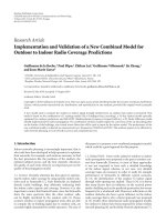
Figure 11: (a): overexposed soundtrack. (b): the corresponding graph: size of structuring element versus normalized volume (sum of gray
values) of the difference between the original image and its successive openings.
Figure 12: Succession of openings with vertical structuring elements and the corresponding differences (between the original image and the
openings).
opening with the same structuring element. The structuring
element is a priori unknown. Given the physical process
that causes overexposure, it can be safely supposed that it
is a disk. Several sizes (limited by the discrete nature of the
scanned soundtrack) should then be tested. However, we can
anticipate that the presence of noise (film grain, dust, etc.)
might interfere in the verification of the hypothesis.
Therefore, we have preprocessed the image of the sound-
track using the method introduced by Brun et al. [12]in
order to binarize it and suppress the noise. The application of
a series of openings with structuring elements of increasing
sizes allows us to check the invariance conjecture. Note that
in the case of soundtracks only containing low-frequency

signals, the invariance is always observed, given that such
tracks do not contain thin structures, whose shape is subject
to variations when overexposed. If a different behavior
exists, it can only be observed in the case of high-frequency
signals. In such cases, we have indeed observed a near-
invariance through a morphological opening, which tends
to confirm our hypothesis (see Figure 11). The detection
of underexposed soundtracks can be done in exactly the
same way, by previously inverting the binary image of the
soundtrack.
A second important feature is that in over-/underexposed
images, the peaks and the valleys have different shapes. The
peaks are sharp and the valleys are hollow or vice versa.
This dissymmetry leads to the fact that the surface of the
peaksisdifferent from that of the valleys. The surface of the
peaks corresponds to the volume of the difference between
the original image and the succession of its morphological
closings with vertical structuring elements of increasing
sizes. Similarly, the surface of the valleys corresponds to the
volume of the difference between the original image and
the succession of its morphological openings with vertical
structuring elements. To illustrate this fact, Figure 12 (resp.,
Figure 13) shows the succession of openings (resp., closings)
with vertical structuring elements of increasing sizes applied
to a soundtrack.
8 EURASIP Journal on Advances in Signal Processing
Figure 13: Succession of closings with vertical structuring elements and the corresponding differences (between the original image and the
closings).
(a)
0

5
10
15
20
25
30
Normalized volume
0123
Size of structuring element
Openings
Closings
(b)
Figure 14: Succession of openings and closings with vertical structuring elements applied to an underexposed soundtrack.
As previously done, we have computed those successions
on our images to obtain the volume of the difference between
the original image and its opening (or closing) in function of
the size of structuring elements. A divergence between the
graph of openings and the one of closings means that the
surfaceofthepeaksisdifferent from that of the valleys and,
therefore, a bad exposure.
Figures 14, 15,and16 show these two graphs for an
underexposed, an overexposed, and a correctly exposed
soundtrack. Notice that, in case of underexposure, the
openings graph is located above the closings one, because
the peaks surface is larger than the valleys one. The inverse
phenomenon is observed in case of underexposure because
the surface of the valleys becomes larger than the one of the
peaks. Finally, because these two surfaces are equal in the
correctly exposed soundtrack, the two graphs are nearly the
same.

Once overexposure has been diagnosed, a correction is
necessary. This could also be done in the image domain using
mathematical morphology. In fact, we have seen that the
detection of the overexposure also produces the size of the
structuring element undergoing in the dilation which models
the overexposure. It will be seen in Section 5.1 how this can
be done.
Only severe under-/overexposition can be discerned by
looking at the optical representation, and only if some
reasonably high-frequency tone is present in the signal. The
grabbed picture shown in Figure 8 shows such oversharp
peaks. This is an extreme case, and for our project, more
gentle distortions should be detected as well. Therefore,
we setup two separate paths in our research planning: one
approach will deal exclusively with the optical representation
of the soundtrack, the second one, described here, will
perform the detection step based onto the audio signal.
4. MEASURING THE DISTORTION IN 1D AUDIO
SIGNAL WITHOUT A PRIORI KNOWLEDGE
As the 1D signal is more or less the transcript of the 2D VA
modulation, a morphological study of the 1D signal shape
will of course make sense, using, for instance, morphological
operators or analysis of local derivatives of the signal.
Jonathan Taquet et al. 9
(a)
0
5
10
15
20

25
Normalized volume
0123
Size of structuring element
Openings
Closings
(b)
Figure 15: Succession of openings and closings with vertical structuring elements applied to an overexposed soundtrack.
(a)
0
5
10
15
20
25
30
35
Normalized volume
0123
Size of structuring element
Openings
Closings
(b)
Figure 16: Succession of openings and closings with vertical structuring elements applied to a correctly exposed soundtrack.
Closely related to 2D image processing, this investigation
is also conducted by Centre de Morphologie Math
´
ematique
(CMM) team.
As stated before, we focus here on the use of 1D

audio signal for the detection and measurement of the
distortion, without reference tone. Motivations are to put
other techniques to work, like frequency analysis and classical
signal processing, to achieve similar results. The correction
itself still takes place in the 2D image representation of the
soundtrack.
We aimed the research toward an indicator able to
determine whether or not a sound sample was distorted
due to incorrect exposure. Since the distortion is frequency
dependant and the recorded sound can be of any nature
(speech, music, etc.), composing a reliable indicator able
to characterize, in an absolute manner, the magnitude of
this distortion seems unrealistic. Therefore, we focused on
a less robust indicator and use it in an iterative process
(Figure 17). The control process operates using the variation
of this indicator (between two iterations) rather than the
instantaneous value of this indicator. This iterative approach
should stop if the variation drops below a defined level;
the amount of iteration is also restricted by the correction
algorithm we use.
Usually, distortion is expressed in relation to a reference
signal. So we first looked for pitch detection to automatically
extract a reference, but we rapidly noticed that this will
be impossible, especially for music. After discarding other
methods (autocorrelation, AMDF [14]), we propose in this
contribution two possible approaches.
10 EURASIP Journal on Advances in Signal Processing
Image
acquisition
Remove noise

in image
Image
correction
(see text)
Image to sound
conversion
Sound
storage
Long term
averaging
Compute
indicator
Graphical
display
Correction parameters
Figure 17: Closed-loop process.
Spectrum-based indicator
As an incorrect exposure introduces more harmonics for the
higher frequencies, one of the considered approaches was to
compute the center of gravity (COG) of spectrum, not only
for the whole spectrum, but piecewise for different frequency
ranges, and to characterize the COG shifts.
Harmonic distortion-based indicator
This indicator should reflect the harmonic distortion
(mainly even harmonics) for supposed fundamental frequen-
cies, if present.
4.1. Distortion detection by center of gravity shifts
The center of gravity of a spectrum (COG) is in a sense,
the “mean” frequency, and this method is used for pitch
detection and for audio restoration [15]. It is calculated by

cog (v)
=
⎧
⎪
⎪
⎪
⎪
⎨
⎪
⎪
⎪
⎪
⎩
0, if
N

n=1
v(n) = 0,

N
n=1
v(n) ×n

N
n
=1
v(n)
, else,
(1)
where v is the output vector (amplitude) from the windowed

DFT at time t. Further, we will use the notation cog (t).
We compute the COG for different ranges, increasing
the amount of high frequencies in the calculation. So we
expect seeing the curves drifting apart if distortion is present.
The COG-shift, which intends to reflect the importance of
under-/overexposure, is computed by summing the distance
between all possible couples of the K COG as
COG-shift
K
(t) =
K

n=1

K

l=n+1


cog (t, n) −cog (t,l)



. (2)
Thus, the method consists in the following steps.
(1) ComputeDFTonthesignalafter removing impulsive
noise in the 2D image representation,
(2) Compute COG over K different ranges of the output
spectrum: [0 1 kHz] [0 2 kHz] [0 6kHz]
[0 12 KHz], therefore, cog (t, k) is the COG that

has been computed at time t of the signal for the
restricted frequency range k,
(3) Compute COG-shift by summing distances b etween
COG results.
Figures 18 and 19 show this behavior. We use our frequency
sweep signal to illustrate the response.
Remark that the COG is related to the spectral slope. For
voice (especially sonorants), the amplitude of the harmonics
falls off 12 dB per octave or more. The shape of this plot is
called the spectral slope. A flatter spectral slope, say around
6 dB/octave, results in stronger high frequencies, which yield
a more “brassy” or strident sound. The steeper the slope, the
lower is the COG. Incorrect exposure of optical soundtrack
introduces harmonics and leads to a more flat plot, therefore,
could also be used as an indicator.
As COG is one of many known techniques for pitch
detection, the ensued indicator somehow follows the pitch
of the sound sample. To be used as feedback value in
our closed-loop approach, a low-pass filtering/averaging has
to be applied to this value. This is not a problem, as
under-/overexposure effect is constant over a long period (a
complete reel, or at least over a shoot, if there are several parts
spliced together on the reel).
Note that noise disturbs this method, especially impul-
sive noise which creates high frequencies, thus rise the COG.
Fortuitously, impulsive noise is easy to remove in the image
domain (dust busting).
4.2. Harmonic distortion approach
Total harmonic distortion (THD) is often used to charac-
terize audio equipment, for example, amplifiers. The main

cause of distortion in amplifiers is the nonlinear behavior
of the gain devices (tubes and transistors) which are part
of the circuit. Experienced audio engineers know that tube
amplifiers often introduces even-order harmonics due to
nonsymmetrical characteristics, and that class-AB amplifier
introduces odd-order harmonics, du to zero crossing and
clipping. This distortion depends on frequency and output
power.
Several THD measures exist, among which the global
total harmonic distortion (THD-G) expresses the power of
a distortion in the signal.
THD-G
f
is the THD-G for the fundamental frequency f :
THD-G
f
(S) =

P
Hk
P
S
,(3)
where P
Hk
is the power of the kth harmonic of the
fundamental frequency f ,andP
S
is the power of the input
signal S.

The analogy to our problem (desymmetrization, clip-
ping) is great enough to undergo a trial; but THD is
Jonathan Taquet et al. 11
0
500
1000
1500
2000
2500
3000
3500
4000
0 5 10 15 20 25
Four spectral COGs of a frequency
sweep for a little overexposure
COG in [0; 6000] Hz
COG in [0; 12000] Hz
COG in [0; 18000] Hz
COG in [0; 24000] Hz
Sweep frequency
(a)
0
500
1000
1500
2000
2500
3000
3500
4000

4500
5000
0 5 10 15 20 25
Four spectral COGs of a frequency
sweep for a more important overexposure
COG in [0; 6000] Hz
COG in [0; 12000] Hz
COG in [0; 18000] Hz
COG in [0; 24000] Hz
Sweep frequency
(b)
Figure 18: (a): COG calculation on the slightly altered sine sweep. All COG plots follow the fundamental frequency. (b): COG calculation
on the sine sweep after simulation of a bad exposure. As expected, the raise of harmonics at increasing frequency shifts the COG to higher
values.
0
500
1000
1500
2000
2500
3000
0 5 10 15 20 25
COG-shift indicator for the frequency sweep
Little overexposure
More important overexposure
(a)
Sound wave
Correct exposure/cog and cog-shift indicator
Overexposure/cog and cog-shift indicator
(b)

Figure 19: (a): COG-shift plotted over time for the frequency-sweep input. As expected, our indicator rises as frequency increase. (b): COG
plot (blue) and COG-shift indicator (black) for a real-sound sample. Even if the variation is small, it is effective over the complete sample.
measured by feeding the equipment with a fixed and known
signal. Measurement is reiterated for varying frequency and
ends with the plot of THD versus input frequency. Since
our signal is recorded without any reference, we thought
about estimating (pitch detection) and measure distortion
relative to it. There are several methods for pitch detection
in literature, but many of these approaches are convenient
to isolate a sine wave from heavy noise, but lot of methods
fail for multitonal music, for example. Because of that,
and inspired by [16], we investigate an ad hoc harmonic
12 EURASIP Journal on Advances in Signal Processing
(a)
0.1
0.12
0.14
0.16
0.18
0.2
0.22
0.24
0 20 40 60 80 100 120 140
Second distorsion indicator for a speech sample
Correctly exposed
With overexposure
(b)
Figure 20: Top left: spectrogram of speech sample (5 seconds), correctly exposed. Bottom left: spectrogram of the same sample after
simulation of overexposure. Right: for this sound sample, the HD-indicator is plotted in black for a correctly exposed soundtrack and
in green for a overexposed one.

distortion indicator. Of course, this indicator will rise for
brass music and get lower for voice, for example, but it has
to reflect the change due to bad exposure for both sounds.
Consequently, our approach consists in the following
steps: the input signal is filtered with a filter bank. Each filter
selects one supposed fundamental frequency. For each one we
compute the energy of its odd and even harmonics up to the
cutoff acquisition frequency (half the sampling frequency),
using two comb filters for this selection.
For the next equations, we will use the following
notations:
(1) s(t): is the value of s at discrete time t,withs(t)
∈
[−1; 1],
(2) s(t
0
, t
n
): are the values of s extracted ranging from t
0
to t
n
,
(3) s
f
(t
0
, t
n
): is the bandpass filtered (centered at f )

signal (used to extract the supposed fundamental
frequency f ),
(4) s
h( f )
(t
0
, t
n
): is the high-pass-filtered (cutoff 1.5 f )
signal given by s
comb ( f )
(t
0
, t
n
), where s
comb ( f )
(t
0
, t
n
)
is the filtered output of s(t
0
, t
n
) by the comb filter
selecting the harmonics of f ;
power of fundamental frequency (FP):
FP

f

s

t
0
, t
n

=
power

s
f

t
0
, t
n

;(4)
harmonics power (HP):
HP
f

s

t
0
, t

n

= power

s
h( f )

t
0
, t
n

;(5)
and the power function is
power

s

t
0
, t
n

=
1
t
n
−t
0
+1

t
n

t=t
0

s(t)

2
. (6)
These supposed fundamental frequencies have been arbitrar-
ily chosen, keeping in mind a future fast IIR implementation.
Moreover, for easy-comb filter design, the rule 2
× f
s
=
f
e
/n should be applied ( f
s
the sampling frequency, f
e
the
supposed fundamental frequency, and n
∈ IN
∗
). Our set
contains the following frequencies (in Hz): 192 240 480 750
1200 1600 2000 3000 4000 4800 6000. Filter design for both
bandpass filters and comb filters has been done thanks to

MATLAB’s filter design tool.
We plot these “harmonic distortion” values against time
for several signals (frequency sweep, voiced signal, music)
before and after alteration by our simulator, we combined
the results in order to find an indicator which reflects the
distortion introduced by a faulty exposure (see Figures 20
and 21).
Harmonic Distortion Indicator HD is null when
power (s(t
0
, t
n
)) = 0, else it is expressed as follow:
HD-indicator

s

t
0
, t
n

=

log
10

1
power (s(t
0

, t
n
))

f ∈filterbank
FP
f

s

t
0
, t
n

HP
f

s

t
0
, t
n


−1
.
(7)
As expressed in (7), the indicator is based on the summa-

tion of the ratio FP
f
(s(t
0
, t
n
))/HP
f
(s(t
0
, t
n
)) for all f
e
∈
filterbank. To avoid high values for signal parts with
little modulation (low frequencies, moments of silence),
Jonathan Taquet et al. 13
0.12
0.14
0.16
0.18
0.2
0.22
0.24
0.26
0.28
0.3
0 20 40 60 80 100
Distorsion indicator for the frequency sweep

Correctly exposed
Little overexposure
More important overexposure
(a)
0.12
0.14
0.16
0.18
0.2
0.22
0.24
0.26
0.28
0.3
0 20 40 60 80 100 120 140
Distorsion indicator for a clarinet
in a concert sound sample
Correctly exposed
With overexposure
(b)
Figure 21: (a): HD-indicator for the frequency sweep test signal (black: correct exposure, green: light overexposure, red: strong
overexposure). (b): HD-indicator for music instrument (clarinet) sample (black: correct exposure, green: light overexposure).
the ratio is weighted by the signal power for this part
(power (s(t
0
, t
n
))). Since power (s(t
0
, t

n
)) ∈ [0; 1], the log 10
scale smooths out abrupt variations. Because we want our
indicator to increase with the distortion, we take the inverse
of this expression.
Even if the behavior of the indicator must be deeper
studied (immunity to noise, linearity, performance for
moments of silence, etc.), using it in the closed-loop scheme
and minimizing it while iterating gave us acceptable results
(given the simple correction we used).
5. CORRECTION OF THE 2D OPTICAL
REPRESENTATION OF THE SOUNDTRACK
A very simple correction was setup to experiment our
“closed-loop” solution. For this, the images are grabbed
with a great dynamic range (our line-scan camera is able to
output 12 bits/pixel) together with a fine tuning of lightning
power and camera integration time. Consequently, we are
able to change the intensity levels of the image pixels over
a great range. For test purposes, we also optically blur
the soundtrack (defocussing the camera). This cuts the
bandwidth, but also enlarges the blending area from black to
white; therefore, the suggested correction is more efficient.
The high dynamic range image is mapped to an 8-
bits/pixel image by following these rules.
(1) The histogram of the 12 bits/pixel image is computed.
The two peaks are detected (corresponding to soundtrack
and surroundings). These grey-levels p
min
and p
max

are used
for the subsequent steps.
(2) A second tone mapping is performed, in form
of a histogram stretching directed by the indicator. The
feedback sign is manually set, since the distortion detection
in the audio signal does not differentiate overexposure
from underexposure. For this histogram stretching, the new
maximum value (resp., minimum, according to feedback
sign) is decreased (resp., increased) by a value (c
p
.indicator)
where c
p
is experimentally set (a complete proportional-
integral-derivative control at each iteration should perform
better, assuming indicator smoothing as well). The output
is shown in Figure 22. The process is reiterated and stopped
after a fixed amount of iterations or if indicator drops below
a threshold. If the amount of iterations is not restricted, the
correction itself stops if minimum reaches (maximum
−1)
(resp., maximum reached (minimum +1)), releasing hence a
binary image.
This simple correction, intended as a proof of concept,
makes use of the image spread (present at photographic level,
emphasized by the slightly blurred acquisition) and shifts the
gray-levels towards black level (resp., towards white level).
Obviously, as the correction is iterated, the image loses in
dynamics and aliasing appears (Figure 23). On the other side,
this kind of correction is really fast (using Look-Up tables).

I
in
: pixel of the 12 bits/pixel image, as grabbed,
I
out
: pixel of a 8 bits/pixel image, used for indicator
calculation,
c
p
:coefficient for the proportionnal term of the regula-
tion loop,
if overexposure: p
min
= p
min
+(c
p
·indicator),
if underexposure: p
max
= p
max
−(c
p
·indicator)
I
out
= (I
in
− p

min
)
b
−a
p
max
− p
min
+ a.
(8)
14 EURASIP Journal on Advances in Signal Processing
(a) (b) (c)
Figure 22: Optical representation of ca. 1/75 second of sound from the “L’acrobate” soundtrack. (a): as grabbed, Middle: histogram
stretching at first iteration, between p
min
and p
max
, (b): after several iterations according to indicator minimization.
(a)
0
0.05
0.1
0.15
0.2
0.25
0.3
0 50 100 150 200 250
(b)
Figure 23: Optical representation of ca. 1/75 second of stereo soundtrack. From left to right: as grabbed, histogram stretching at first iteration
(based on histogram), 2nd, 3th, and 4th iteration. Below: plot of the HD indicator value versus p

min
. The HD indicator values for this plot is
the mean value computed on 64000 samples (1,33 seconds).
5.1. Correction by mathematical morphology
Considering real data, especially the “L’acrobate” soundtrack
(opening credits music from the movie “L’acrobate” (1940)),
the visual examination of the acquired images advise us that
a simple correction based on a transfer function should not
be sufficient.
We have su pp os ed in Section 3 that overexposure can be
modelled as a morphological dilation, and we have explained
how to validate this hypothesis and compute the size of the
corresponding structuring element. If this hypothesis is true,
then the theory of mathematical morphology tells us that
some information might have been lost in the process, and
that a good candidate for the restoration is obtained with a
morphological erosion using the same structuring element.
Underexposed soundtracks would be restored analogously by
using a dilation.
6. CONCLUSION AND FORTHCOMING WORK
Validation has been performed on simulated data but also
on real data, but for the latter, we do not hold any unaltered
Jonathan Taquet et al. 15
(a)
−10.5
−10
−9.5
−9
−8.5
−8

−7.5
−7
0 200 400 600 800 1000
Distorsion indicator for a real case 0.1, 0.005
Correction trial
Original
(b)
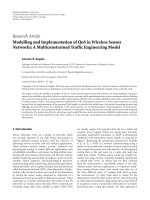
Figure 24: Top left: spectrogram of real soundtrack (“L’acrobate,” 5 seconds), grabbed by our scanner and converted to sound. Bottom left:
spectrogram of the same sample after correction. Notice the noise level for real soundtracks (here no dust removal was performed). Right:
for this sound sample, the HD-indicator is plotted in green before correction and in black after correction.
400 Hz reference
Original undistorted x-modulation signal
Distorted x-modulation signal
Filtered 400Hz component
of distorted x-modulation signal
(a)
(b)
Figure 25: (a): graphical illustration of the cross-modulation test (lifted from Kodak’s technical note “cross-modulation distortion testing
for the motion picture laboratory”). (b): image grabbed from a real cross-modulation test reel (stereo tracks).
counterpart to compare with. The results look promising, to
be said that it is easier at this stage to do a visual assessment
of the restored images or compare spectrograms (Figure 24)
rather than listening to the converted sound.
Using pure image processing for detecting this impair-
ment involves operators which are noise sensitive, especially
dust located near the “black to white” transitions. A perfect
digital cleaning of the tracks is a tedious process, up to now
too slow for implementation, and the related research on
this process is out of the topic of this paper. Hence, our
proposal to use signal processing in the audio domain for

distortion detection makes sense and is easier, since the way
the soundtracks are read (integration over a line) minimizes
the incidence of dust.
On the contrary, using image-based correction seems to
be mandatory. The simple correction scheme used for the
proof of concept (adjusting the luminance distribution) is
interesting because it is simple and related to the steepness of
the grey-level slope in area where image spread occurs. How-
ever, for high degrees of incorrect exposure, the correction
will need support of more complex operators. This will be a
forthcoming work.
Both indicators seem valuable, but the COG-shift is too
sensitive to noise present in moment of silence (MOS).
16 EURASIP Journal on Advances in Signal Processing
Nevertheless, both indicators tend to follow the pitch,
therefore, settings the rights coefficientinaPIDregulation
scheme and adjusting the window sizes for FFT and filtering
have to be investigated.
Opening up an unmarked application field, the solution
proposed is very innovative in its construction by coupling
signal processing and image processing in a regulation loop.
A valuable simulation framework has been set up, and
some methods have been investigated to extract an indicator
reflecting the distortion caused by under-/overexposure
without prior knowledge. The open loop behavior of indi-
cator (S) needs to be more deeply investigated (monotony,
linearity, etc.).
The presented work (computation of indicators, simple
correction) is about to be coded in real time, using Intel
performance primitives (IPP), as a computing stage closely

coupled to the image acquisition stage of the RESONANCES
soundtrack scanner.
At last, as an absolute improvement is hard to perceive
while listening to a real-altered sound sample, comparative
listening will be meaningful for the sound samples and their
simulated degraded duplicate. Blindfold listening test at a
postprocessing auditorium is planned.
APPENDIX
THE CROSS-MODULATION TEST
Soon after the introduction of optical soundtracks in the
movie industry, the processing labs asked for a procedure
to determine the optimum exposure conditions for both
negative and print. From the forties forward, an industry-
standard practice raised, commonly known as the “cross-
modulation test,” and is still used as a quality assurance
routine prior to sound recording and duplication. The test is
based on the fact that a perfect sinusoid comprising a high-
frequency signal (about 10 kHz) modulated at 75% by a low-
frequency one (typically 400 Hz) will have an average value
of zero (the average light transmission will be constant). In
the case of underexposure or overexposure, some of the low-
frequency modulation component will be introduced into
the average value of the signal and may be detected. Figure 25
illustrates this process. A low-pass filter is connected after the
optical pickup head to eliminate the high-frequency carrier,
and the amount of 400 Hertz signal remaining is analyzed to
determine the exposure and printing conditions which result
in the lowest-level signal. That means a technician reads a
simple needle display showing the average level and graphs
values against processing parameters.

This technique is still used and we suggest the eager
readers to study further the technical note from Kodak [17]
on the cross-modulation test.
ACKNOWLEDGMENTS
This work was made possible thanks to the financial help
of the French AgenceNationaledelaRecherche, through its
RIAM program. The film material, as well as the expertise
on motion picture optical soundtracks, were provided by N.
Ricordel from the CNC—Archives Franc¸aises du Film and by
C. Comte from GTC-Eclair Group.
REFERENCES
[1] E. W. Kellog, “History of sound motion pictures,” Journal of
the SMPTE, vol. 64, pp. 291–302, 1955.
[2] J. G. Frayne and H. Wolfe, Sound Recording, John Wiley &
Sons, New York, NY, USA, 1949.
[3] Erpi ClassRoom Films Inc., Sound recording and reproduc-
tion (sound on film). An instructional sound film, 1943,
/>[4] J. Monaco, How to Read a Film, Oxford University Press,
Oxford, UK, 3rd edition, 2000.
[5] “Cinematography—A-chain frequency response for repro-
duction of 35 mm photographic sound—Reproduction char-
acteristics,” International Norm ISO 7831, 1986.
[6] P. Streule, Digital image based restoration of optical movie sound
track, M.S. thesis, Electronics Labs, Swiss Federal Institute of
Technology, Zurich, Switzerland, March 1999.
[7] D. Richter, D. Poetsch, and A. Kuiper, “Localization of faults
in multiple double sided variable area code sound tracks
on motion picture films using digital image processing,” in
Proceedings of the 13th International Czech - Slovak Scientific
Conference Radioelektronika, Brno, Czech Republic, May 2003.

[8] D. Poetsch, D. Richter, and I H. Kurreck, “Restoration of
optical variable density sound tracks on motion picture
films by digital image processing,” in Proceedings of the
International Conference on Optimization of Electrical and
Electronic Equipments (OPTIM ’00), pp. 793–798, Brasov,
Romania, May 2000.
[9] A. Kuiper and L. Dzbnek, “Localization of faults in multiple
double sided variable area sound tracks on motion picture
films using digital image processing,” Departement of Radio
Electronics, FEEC, BUT, 2005.
[10] A. Kuiper, “Detection of dirt blotches on optical soundtracks
using digital image processing,” in Proceedings of the 15th Inter-
national Czech - Slovak Scientific Conference Radioelektronika,
Brno, Czech Republic, May 2005.
[11] J. Valenzuela, “Digital audio image restoration: introducing a
new approach to the reproduction and restoration of analog
optical soundtracks for motion picture film,” in Proceed-
ings of the Internat ional Broadcasting Convention (IBC ’03),
Technicolor Creative Services, Amsterdam, The Netherlands,
September 2003.
[12] E. Brun, A. Hassaine, B. Besserer, and E. Decenciere, “Restora-
tion of variable area soundtracks,” in Proceedings of the IEEE
International Conference on Image Processing (ICIP ’07),pp.
13–16, San Antonio, Tex, USA, September 2007.
[13] J. Serra, Image Analysis and Mathematical Morphology, vol. 1,
Academic Press, London, UK, 1982.
[14] G. S. Ying, L. H. Jamieson, and C. D. Michell, “Probabilistic
approach to AMDF pitch detection,” in Proceedings of the
4th International Conference on Spoken Language Processing
(ICSLP ’96), vol. 2, pp. 1201–1204, Philadelphia, Pa, USA,

October 1996.
[15] A. Czyzewski and P. Maziewski, “Some techniques for wow
effect reduction,” in Proceedings of the IEEE International
Conference on Image Processing (ICIP ’07), vol. 4, pp. 29–32,
San Antonio, Tex, USA, September 2007.
Jonathan Taquet et al. 17
[16] R. A. Irizarry, “Local harmonic estimation in musical sound
signals,” Journal of the American Statistical Association, vol. 96,
no. 454, pp. 357–367, 2001.
[17] “Cross-modulation distortion testing for the motion picture
laboratory,” Tech. Rep., Eastman Kodak Company, Rochester,
NY, USA, 2001, />en/motion/support/h44/h44.pdf.