Báo cáo hóa học: " Research Article Flicker Compensation for Archived Film Sequences Using a Segmentation-Based Nonlinear Model" doc

Hindawi Publishing Corporation
EURASIP Journal on Advances in Signal Processing
Volume 2008, Article ID 347495, 16 pages
doi:10.1155/2008/347495
Research Article
Flicker Compensation for Archived Film Sequences Using
a Segmentation-Based Nonlinear Model
Guillaume Forbin and Theodore Vlachos
Centre for Vision, Speech and Signal Processing, University of Surrey, GU2 7XH, Guildford, Surrey, UK
Correspondence should be addressed to Guillaume Forbin,
Received 28 September 2007; Accepted 23 May 2008
Recommended by Bernard Besserer
A new approach for the compensation of temporal brightness variations (commonly referred to as flicker) in archived film
sequences is presented. The proposed method uses fundamental principles of photographic image registration to provide
adaptation to temporal and spatial variations of picture brightness. The main novelty of this work is the use of spatial segmentation
to identify regions of homogeneous brightness for which reliable estimation of flicker parameters can be obtained. Additionally
our scheme incorporates an efficient mechanism for the compensation of long duration film sequences while it addresses problems
arising from varying scene motion and illumination using a novel motion-compensated grey-level tracing approach. We present
experimental evidence which suggests that our method offers high levels of performance and compares favourably with competing
state-of-the-art techniques.
Copyright © 2008 G. Forbin and T. Vlachos. This is an open access article distributed under the Creative Commons Attribution
License, which permits unrestricted use, distribution, and reproduction in any medium, provided the original work is properly
cited.
1. INTRODUCTION
Flicker refers to random temporal fluctuations in image
intensity and is one of the most commonly encountered
artefacts in archived film. Inconsistent film exposure at the
image acquisition stage is its main contributing cause. Other
causes may include printing errors in film processing, film
ageing, multiple copying, mould, and dust.
Film flicker is immediately recognisable even by nonex-

pert viewers as a signature artefact of old film sequences.
Its perceptual impact can be significant as it interferes
substantially with the viewing experience and has the
potential of concealing essential details. In addition it
can be quite unsettling to the viewer, especially in cases
where film is displayed simultaneously with video or with
electronically generated graphics and captions as is typically
the case in modern-day television documentaries. It may
also lead to considerable discomfort and eye fatigue after
prolonged viewing. Camera and scene motion can partly
mask film flicker and as a consequence, the latter is much
more noticeable in sequences consisting primarily of still
frames or frames with low-motion content. In addition
it must also be pointed out that inconsistent intensity
between successive frames reduces motion estimation accu-
racy and by consequence the efficiency of compression
algorithms.
Flicker has often been categorised as a global artefact
in the sense that it usually affects all the frames of a
sequence in their entirety as opposed to so-called local
artefacts such as dirt, dust, or scratches which affect a limited
number of frames and are usually localised on the image
plane. Nevertheless it is by no means constant within the
boundaries of a single frame as explained in the next section
and one of the main aims of this work is to address this issue.
1.1. Spatial variability
Flicker can be spatially variable and can manifest itself in
any one of the following ways. Firstly, when flicker affects
approximately the same position of all the frames in a
sequence. This may occur directly during film shooting if

scene lighting is not synchronised with the shutter of the
camera. For example, if part of the scene is illuminated with
synchronised light while the rest is illuminated with natural
light a localised flickering effect may occur. This can also be
due to fogging (dark areas in the film strip) which is caused
2 EURASIP Journal on Advances in Signal Processing
B
C
D
A
(a)
100500
Frame number
130
175
220
Median value of the patches
Block A
Block B
Block C
Block D
(b)
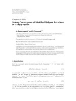
Figure 1: (a) Test sequence Boat used to illustrate spatial variability
of flicker measured at selected location. (b) Evolution of the median
intensity of the selected blocks.
by the accidental exposure of film to incident light, partial
immersion or the use of old or spent chemicals on the film
strip in the developer bath. Drying stains from chemical
agents can also generate flicker [1–6].
It is also possible that flicker localisation varies randomly.

This is the case when the film strip ages badly and becomes
affected by mould, or when it has been charged with static
charge generated from mechanical friction. The return to a
normal state often produces static marks.
Figure 1 shows the first frame of the test sequence Boat
(Our Shrinking World (1946) - Young America Films, Inc. -
Sd, B&W. (1946)). The camera lingers in the same position
during the 93 frames of the sequence. There is also some
slight unsteadiness. Despite some local scene motion, overall
motion content is low. This sequence is chosen to illustrate
that the spatial variation of flicker is not perceivable on the
top-left part of the shot, while the bottom-left part changes
from brighter initially to darker later on. On the right-hand
side of the image, flicker is more noticeable, with faster
variations of higher amplitude. This is shown in Figure 1,
where the median intensities of four manually selected blocks
(16
× 16 pixels) located at different parts of the frame are
plotted as a function of frame number.
The selected blocks are motionless, low-textured and
have pairwise similar grey levels (A, B and C, D) at the start of
the sequence. As the sequence evolves we can clearly observe
that each block of a given pair undergoes a substantially
different level of flicker with respect to the other block. This
example also illustrates that flicker can affect only a temporal
segment of a sequence. Indeed, from the beginning of the
shot to frame 40 the evolution of the median intensities for
blocks A and B is highly similar, thus degradation is low
compared to the segment that follows the first 40 frames.
This paper introduces two novel concepts for flicker

compensation. Firstly, the estimation of the flicker com-
pensation profile is performed on regions of homogeneous
intensity (Section 4). The incorporation of segmentation
information enhances the accuracy and the robustness of
flicker estimation.
Secondly, the concept of grey-level tracing (developed
in Section 5) is a fundamental mechanism for the correct
estimation of flicker parameters as they evolve over time.
Further, this is integrated into a motion-compensated,
spatially-adaptive algorithm which also incorporates the
nonlinear modelling principles proposed in [7, 8]. It is
worth noting that [7] is a proof-of-concept algorithm that
was originally designed to compensate frame pairs but was
never engineered as a complete solution for long-duration
sequences containing arbitrary camera and scene motion,
intentional scene illumination changes, and spatially varying
flicker effects.
This is demonstrated in Figure 2 where the algorithm in
[7] achieves flicker removal by stabilising the global frame
intensity over time but only with respect to the first frame
of the sequence which is used as a reference. In contrast the
proposed algorithm is well-equipped to deal with motion,
intentional illumination fluctuations and spatial variations
and, together with a shot change detector, it can be used as
a complete solution for any sequence irrespective of content
and length.
This paper is organised as follows. Section 2 reviews the
literature of flicker compensation while Section 3 provides
an overview of our previous baseline approach based on
a nonlinear model and proposed in [7]. Improvements

reported in [8] and related to the flicker compensation pro-
file estimation are presented in Sections 3.2 and 3.3.Spatial
adaptation and incorporation of segmentation information
are described in Section 4. Finally, a temporal compen-
sation framework using a motion-compensated grey-level
tracing approach is presented in Section 5 and experimental
results are presented in Section 6. Conclusions are drawn in
Section 7.
2. LITERATURE REVIEW
Flicker compensation techniques broadly fall into two cate-
gories. Initial research addressed flicker correction as a global
compensation in the sense that an entire frame is corrected
in a uniform manner without taking into account the spatial
G. Forbin and T. Vlachos 3
1009080706050403020100
Frame number
80
85
90
95
100
105
110
115
120
125
130
135
Mean frame intensity for test sequence “boat”
Original

Baseline
Proposed
Figure 2: Comparison of mean frame intensity as a function of time
between the original, the baseline scheme [7, 8] and the proposed
approach.
variability issues illustrated previously. More recent attempts
have addressed spatial variability.
2.1. Global compensation
Previous research has frequently led to linear models where
the corrected frame was obtained by linear transformation
of the original pixel values. A global model was formulated
which assumed that the entire degraded frame was affected
with a constant intensity offset. In [1], flicker was modelled
as a global intensity shift between a degraded frame and the
mean level of the shot to which this frame belongs. In [2],
flicker was modelled as a multiplicative constant relating the
mean level of a degraded frame to a reference frame. Both
the additive and multiplicative models mentioned above
require the estimation of a single parameter which although
straightforward fails to account for spatial variability.
In [3] it was observed that archive material typically has
a limited dynamic range. Histogram stretching was applied
to individual frames allowing the available dynamic range to
be used in its entirety (typically [0 : 255] for 8 bits per pixel
image). Despite the general improvement in picture quality
the authors admitted that this technique was only moderately
effective as significant residual intensity variations remained.
The concept of histogram manipulation has been further
explored in [1] where degradation due to flicker was mod-
elled as a linear two-parameters grey-level transformation.

The required parameters were estimated under the constraint
that the dynamic range of the corresponding non-degraded
frames does not change with time.
Work i n [ 4, 9] approached the problem using histogram
equalisation. A degraded frame was first histogram-equalised
and then inverse-histogram was performed with respect
to a reference frame. Inverse equalisation was carried out
in order for the degraded frame to inherit the histogram
profile of the reference. Our previous work described in
[7] used non-linear compensation motivated by principles
of photographic image registration. Its main features are
summarised in Section 3.1. Ta bl e 1 presents a brief overview
of global compensation methods.
2.2. Spatially-adaptive compensation
Recent work has considered the incorporation of spatial
variability into the previous models. In [5] a semi-global
compensation was performed based on a block-partitioning
of the degraded frame. Each block was assumed to have
undergone a linear intensity transformation independent
of all other blocks. A linear minimum mean-square error
(LMMSE) estimator was used to obtain an estimate of the
required parameters. A block-based motion detector was
also used to prevent blocks containing motion to contribute
to the estimation process and thus the missing parameters
due to the motion were interpolated using a successive
over-relaxation technique. This smooth block-based sparse
parameter field was bi-linearly interpolated to yield a dense
pixel-accurate correction field.
Research carried out in [10, 11] has extended the global
compensation methods of [1, 2] by replacing the additive

and multiplicative constants with two-dimensional second-
order polynomials. It matches the visual impression one
gets by inspecting actual flicker-impaired material. In [10]a
robust hierarchical framework was proposed to estimate the
polynomial functions, ranging from zero-order to second-
order polynomials. Parameters were obtained using M-
estimators minimising a robust energy criterion while lower-
order parameters were used as an initialisation for higher-
order ones. Nevertheless, it has to be pointed out that the
previous estimators were integrated in a linear regression
scheme, which introduces a bias if the frames are not
entirely correlated (regression “fallacy” or regression “trap”
[12], demonstrated by Galton [13]). In [11]analternative
approach to the parameter estimation problem which tried
to solve this issue was proposed. A histogram-based method
[6] was formulated later on and joint probability density
functions (pdfs) (establishing a correspondence between
grey levels of consecutive frames) were estimated locally
in several control points using a maximum-a-posteriori
(MAP) technique. Afterwards a dense correction function
was obtained using interpolation splines. The same authors
proposed recently in [14] a flicker model able to deal
within a common framework with very localised and smooth
spatial variations. Flicker model is parametrised with a
single parameter per pixel and is able to handle non-
linear distorations. A so-called “mixing model” is estimated
reflecting both the global illumination of the scene and the
flicker impact.
A method suitable for motionless sequences was
described in [15]. It was based on spatiotemporal segmen-

tation, the main idea being the isolation of a common
background for the sequence and the moving objects. The
background was estimated through a regularised average
4 EURASIP Journal on Advances in Signal Processing
Table 1: An overview of the global flicker compensation techniques.
Global compensation techniques Summary
Wu and Suter [1] linear compensation—flicker is modelled as a global intensity shift.
Decenci
`
ere [2] linear compensation—flicker is modelled as a multiplicative constant.
Richardson and Suter [3]
histogram-based compensation—histogram stretching across the avail-
able greyscale.
Wu and Suter [1]
histogram-based compensat ion—histogram stretching across the refer-
ence frame greyscale.
Schallauer et al. [9] and Naranjo and Albiol [4]
histogram-based compensation—histogram equalisation with respect
to a reference frame.
Vlachos [7]
Non-linear approach: flicker parameters are estimated independently
for each grey-level and a compensation profile is obtained.
Table 2: An overview of the spatially adaptive compensation techniques.
Spatially adaptive compensation techniques Summary
van Roosmalen et al. [5]
Linear compensation: block-partitioning of the degraded frame.
Smoothing of the sparse parameter field.
Ohuchi et al. [10]
Linear compensat ion : flicker is modelled as 2-parameter 2nd order
polynomials, hierarchical parameters estimation.

Kokaram et al. [11]
Linear compensat ion : flicker is modelled as 2-parameter 2nd order
polynomials, parameters estimation based on an unbias linear
regression.
Jung et al. [15]
Linear compensation: spatio-temporal segmentation isolating the
background and the moving objects. Temporal average of the grey
levels preserving the edges to reduce the flicker.
Piti
´
eetal.[6]
Histogram-based compensation: Joint probability density functions
(pdfs) estimated locally in several control points. Dense correction
function obtained using interpolation splines.
Forbin et al. [8]
Non-linear formulation: block-partionning of the degraded frame and
estimation of intensity error profiles on each blocks using motion-
compensated frame. Non-linear Interpolation of the compensation
values weighted by estimated reliabilities.
Piti
´
eetal.[14]
Pixel-based flicker estimation: flicker strength is estimated for each
pixel using a “mixing model” of the global illumination.
(preserving the edges) of the sequence frames, while moving
objects were motion compensated, averaged and regularised
to preserve spatial continuities. Tab le 2 presents a brief
overview of the above methods.
Based on the nonlinear model formulated in [7],
we proposed significant enhancement towards a motion-

compensation-based spatially-adaptive model [8]. These
improvements are extensively detailed in Sections 3.2, 3.3,
and 4.1.
2.3. Compensation for sequences of longer duration
While the above efforts addressed the fundamental esti-
mation problem with varying degrees of success far fewer
attempts were made to formulate a complete and integrated
compensation framework suitable for the challenges posed
by processing longer sequences. In such sequences the main
challenges relate to continuously evolving scene motion
and illumination rendering considerably more difficult the
appointment of reference frames. In [9] reference frames
were appointed and a linear combination of the inverse
histogram equalisation functions of the two closest reference
frames (forward/backward) was used for the compensation.
In [4] a target histogram was calculated for histogram
equalisation purposes by averaging neighbouring frames’
histograms within a sliding window. This technique was also
used in [16], but there the target histogram was defined as
a weighted intermediary between the current frame and its
neighbouring histograms, the computation being inspired
from scale-time equalisation theory.
In [5] compensation was performed recursively. Error
propagation is likely in this framework as previously gen-
erated corrections were used to estimate future flicker
parameters. A bias was introduced and the restored frame
was a mixture of the actual compensated frame and the
original degraded one. In [11, 14] an approach motivated
by video stabilisation described in [2] is proposed. Several
flicker parameter estimations are computed for a degraded

G. Forbin and T. Vlachos 5
frame within a temporal window and an averaging filter
is employed to provide a degree of smoothing of those
parameters.
3. NONLINEAR MODELLING
This section summarises our previous work reported in [7],
which addressed the problem using photographic acquisition
principles leading to a nonlinear intensity error profile
between a reference and degraded frame. The proposed
model assumes that flicker is originated from exposure
inconsistencies at the acquisition stage. Quadratic and cubic
models are provided, which means that the method is
able to compensate for other sources of flicker respecting
these constraints. Important improvements are discussed in
Sections 3.2 and 3.3.
3.1. Intensity error profile estimation based on
the Density versus log-Exposure characteristic
The Density versus log-Exposure characteristic D(log E)
attributed to Hurter and Driffield [17](Figure 3) is used
to characterise exposure inconsistencies and their associated
density errors.
The slope of the linear region is often referred to
as gamma and defines the contrast characteristics of the
photosensitive material used for image acquisition. In [7]
it was shown that an observed image intensity I with
underlying density D and associated errors ΔI and ΔD due
to flicker are related via
I
−→ ΔI,(1)
which can as well be expressed by

exp(
−D) −→ ΔD·exp(−D). (2)
The mapping I
→ ΔI relates grey-level I in the reference
image and the intensity error ΔI in the degraded image.
In other words, this mapping determines the amount of
correction ΔI to be applied to a particular grey-level I
in order to undo the flicker error. As the Hurter-Driffield
characteristic is usually film stock dependent and hence
unknown, D and ΔD are difficult to obtain. Nevertheless an
intensity error profile ΔI across the entire greyscale can be
estimated numerically. Figure 3 shows a typical such profile
which is highly non-linear, concave, peaking at the midgrey
region and decreasing at the extremes of the available
scale, as plotted in Figure 4. As a consequence, a quadratic
polynomial could be chosen to approximate the intensity
error profile in a parametrised fashion. Nevertheless, telecine
grading (contrast, greyscale linearity, and dynamic range
adjustments performed during film-to-video transfer) can
introduce further non-linearity as discussed in [7]anda
cubic polynomial approximation is more appropriate in
those cases.
An intensity error profile ΔI
t,ref
is determined between
a reference and a degraded frame F
ref
and F
t
,respectively,

where I
ref
and I
t
= I
ref
− ΔI
t,ref
(I
t
) are grey levels of co-sited
pixels in the reference and degraded frames and ΔI
t,ref
(I
t
)is
420
log (exposure)
0
1.5
3
Density
Exposure error
Density error
Figure 3: Hurter-Driffield D(log E) characteristic (dashed) and
density error curve (solid) due to exposure inconsistencies.
2501250
Intensity
0
7

14
Intensity error
Figure 4: Theoretical intensity error profile as a function of
intensity (all units are grey-levels).
the flicker component for grey-level I
t
. For monochrome 8-
bits-per-pixel images, I
t
, I
ref
∈{0, 1, , 255}.Thiscompen-
sation profile allows to reduce F
t
flicker artefact according
to F
ref
. In this framework, F
ref
is chosen arbitrarily, as a
nondegraded frame is usually not available. It is assumed that
motion content between those two images is low and does
not interfere in the calculations. To estimate ΔI
t,ref
(I
t
), pixel
differences between all pixels with intensity I
t
in the degraded

frame and their cosited pixels in position

p
= (x, y) in the
reference frame are computed and a histogram H
t,ref
(I
t
)of
the error is compiled as follows:
∀F
t


p

= I
t
: H
t,ref

I
t

= hist

F
t



p

−F
ref


p

. (3)
6 EURASIP Journal on Advances in Signal Processing
300−30
Intensity difference
0
125
250
Number of occurrences
Greylevel = 50
(a)
300−30
Intensity difference
0
125
250
Number of occurrences
Greylevel = 60
(b)
Figure 5: Intensity difference histograms H
t,ref
(50) and H
t,ref

(60) and their maxima for two consecutive frames of test sequence Caption.
An example is shown in Figure 5 for the test sequence
Caption and two sample grey levels. The intensity error is
given by
ΔI
t,ref

I
t

=
arg max

H
t,ref

I
t

. (4)
The process is repeated for each intensity level I
t
to
compile an intensity error profile for the entire greyscale.
As the above computation is obtained from real images, the
profile ΔI
t,ref
is unlikely to be smooth and is likely to contain
noisy measurements. Either a quadratic or cubic polynomial
least-squares fitting can be applied to the compensation

profile. Cubic approximation is more complex and more
sensitive to noise but is able to cope with nonlinearity
originated from telecine grading, as discussed in [7]:

A
= arg min

I
t

P
t,ref

I
t

−
ΔI
t,ref

I
t

2
,
with

A
=


a
0
, , a
L

, P
t,ref

I
t

=
L

k=0
a
k
·I
k
t
.
(5)
L being the polynomial order. An example is shown
in Figure 4. Finally the correction applied to the pixel at
location

p is:
F

t



p

= F
t


p

+ P
t,ref

F
t


p

. (6)
3.2. Grey-level intensity error reliability weighting
The first important improvement to the baseline scheme in
[7] is motivated by the observation that taking into account
the frequency of occurrence of grey-levels can enhance the
reliability of the estimation process. This enhancement is
presented in [8]. grey-levels with low pixel representation
should be less relied upon and vice versa. In addition,
ΔI
t,ref
estimation accuracy can vary for different intensities

as illustrated in Figure 5. It can be seen for example that
H
t,ref
(50) is spread around an intensity error of 15 and even
if the maximum is reached for 12, many pixels actually
voted for a different compensation value. On the other hand
the strength of consensus (i.e., height of the maximum)
of H
t,ref
(60) suggests a more unanimous verdict. Thus the
reliability of ΔI
t,ref
depends on the frequency of I
ref
but also
on H
t,ref
. A weighted polynomial least square fitting [18]
is then used to compute the intensity error profile and the
weighting function reflecting grey-level reliability is chosen
as:
r
t,ref

I
t

=
max


H
t,ref

I
t

. (7)
Indeed, if I
t
does not occur very frequently in F
t
then
r
t,ref
(I
t
) will be close to 0 and reliability will be influenced
accordingly. The polynomial C
t,ref
parameters are now
obtained as the solution to the following weighted least-
squares minimisation problem:

A

= arg min

I
t
r

t,ref

I
t

·

C
t,ref

I
t

−
ΔI
t,ref

I
t

2
. (8)
An example of reliability distribution r
t,ref
is shown at
the bottom of Figure 6, and highlights that pixel intensities
above 140 are poorly represented. A comparison between the
resulting unweighted correction profile P
t,ref
(dashed line)

and the improved one C
t,ref
(solid line) confirms that more
densely populated grey-levels have a stronger influence on
the fidelity of the fitted profile.
A side benefit of this enhancement is that it allows
our scheme to deal with compressed sequences such as
MPEG material. The quantisation used in compression
may obliterate certain grey levels. An absent grey-level I
t
implies that H
t,ref
(I
t
) = 0, thus r
t,ref
(I
t
) = 0, which
means that ΔI
t,ref
(I
t
) will not be used at all in the fitting
process.
3.3. Motion compensated intensity error
profile estimation
Theaboveworkswellifmotionvariationsbetweenarefer-
ence and a degraded frame are low. As stated in [8], motion
compensation must be employed to be able to cope with

longer duration sequences. This will enable the estimation
of a flicker compensation profile between a degraded- and
a motion-compensated reference frame F
c
t,ref
.Inourwork
we use the well-known Black and Anandan dense motion
estimator [19]asitiswellequippedtodealwiththeviolation
G. Forbin and T. Vlachos 7
2001000
−10
30
Intensity error
(a)
2001000
Intensity
0
1
Reliability
(b)
Figure 6: Measured and polynomial approximated (dashed:basic
fitting - solid:weighted fitting) intensity error profiles as a function
of intensity between the first two frames of test sequence Capt ion.
A quadratic model is used. The histogram below shows the
normalised confidence values r
t,ref
for each grey-level.
of the brightness constancy assumption, which is a defining
feature of flicker applications. Other dense or sparse motion
estimators can be used depending of robustness and speed

requirements. Robustness is crucial as incorrect motion
estimation will fail the flicker compensation. The motion
compensation error will provide a key influence towards
intensity error profile estimation. Indeed, (3) attributes the
same importance to each pixel contributing to the histogram.
The motion compensation error is employed to decrease the
influence of poorly compensated pixels. This is achieved by
compiling H
c
t,ref
(I
t
) using real-valued (as opposed to unity)
increments for each pixel located at

p (i.e., F
t
(

p ) = I
t
)
according to the following relationship:
e
c
t,ref


p


=
1 −


E
c
t,ref


p



max



E
c
t,ref


p




,(9)
E
c

t,ref
being the motion prediction error, that is, E
c
t,ref
= F
c
ref
−
F
t
.Thuse
c
t,ref
(

p ) varies between 0 and 1 and is inversely
proportional to E
c
t,ref
(

p ), and so high confidence is placed on
pixels with a low motion compensation error and vice versa.
In other words, areas where local motion can be reliably
predicted (hence yielding low levels of motion compensation
error) are allowed to exert high influence on the estimation
of flicker parameters. Pixels with poorly estimated motion,
on the other hand, are prevented from contributing to the
flicker correction process.
4. SPATIAL ADAPTATION

The above compensation scheme performs well if the
degraded sequence is globally affected by flicker artefact.
However, as illustrated in Section 1.1 this is not always the
case. Spatial adaptation is achieved by taking into account
regions of homogeneous intensity. The incorporation of
segmentation information enhances the accuracy and the
robustness of flicker parameters estimation.
4.1. Block-based spatial adaptation
Spatial adaptation requires mixed block-based/region-based
frame partitioning. The block-based part is illustrated in
Figure 7.CorrectionprofilesC
t,ref,b
are computed indepen-
dently for each block b of frame F
t
. As brute force correction
of each block would lead to blocking artefacts at block
boundaries (Figure 8), a weighted bilinear interpolation is
used.
It is assumed initially that flicker is spatially invariant
within each block. For each block a correction profile is
computed independently between I
ref
and I
t
, yielding values
for ΔI
t,ref,b
, C
t,ref,b

and r
t,ref,b
, b = [1; B], b being the block
index and B the total number of blocks.
Blocking is avoided by applying bilinear interpolation
of the B available correction values C
t,ref,b
(F
t
(

p )) for pixel

p. Interpolation is based on the inverse of the Euclidean
distance c
b
(

p ) =

(x − x
b
)
2
+(y − y
b
)
2
,
d

b


p

=
1
c
b


p

+1
(10)
with (x
b
, y
b
) being the coordinates of the centre of the block
b for which the block-based correction derived earlier is
assumedtoholdtrue.
This interpolation smooths the transitions across blocks
boundaries. In addition, reliability measurements r
t,ref,b
of
C
t,ref,b
detailed in Section 3.2 are also used as a second
weight in the bilinear interpolation. This allows to discard

measurements coming from blocks where F
t
(

p )ispoorly
represented. Polynomial approximation on blocks with a
low grey-level dynamic will only be accurate on a narrow
part of the greyscale, but rather unpredictable for absent
grey levels. r
t,ref,b
is employed to lower the influence of
such estimation. Intensity error estimation C
t,ref,b
are finally
weighted by the product of the two previous terms, giving
equal influence to distance and reliability. In general it is
possible to apply unequal weighting. If the distance term is
favoured unreliable compensation values will degrade the
quality of the restoration. If the influence of the distance
term is diminished, blocking artefacts will emerge as shown
in Figure 8. It has been experimentally observed that equal
8 EURASIP Journal on Advances in Signal Processing
C
t,R,1
(F
t
(
−→
p ))
r

t,R,1
(F
t
(
−→
p ))
C
t,R,9
(F
t
(
−→
p ))
r
t,R,9
(F
t
(
−→
p ))
C
t,R,3
(F
t
(
−→
p ))
r
t,R,3
(F

t
(
−→
p ))
Figure 7: Block-based partition of the first frame of Boat using a 3×3 grid. The pixel undergoing compensation and the centre of each block
are represented by black and white dots, respectively. The black lines represent the Euclidean distances c
b
(p). Polynomial correction profiles
C
t,ref,b
and associated reliabilities r
t,ref,b
are available for each block b. Compensation value for pixel

p is obtainted by a bilinear interpolation of
the block-based compensation values (9 in this example). Bilinear interpolation involves weighting by block-based reliabilities and distances
d
b
.
(a) (b)
Figure 8: (a) Compensation of the frame 20 of the test sequence Boat applied independently on each block of a 3 × 3 grid. As expected
blocking artefacts are visible. (b) Compensation using the spatially adaptive version of the algorithm.
weights provide a good balance between the two. The final
correction value is then given by
F

t


p


= F
t


p

−
B

b=1

d
b


p

·r
t,ref,b

F
t


p

·C
t,ref,b


F
t


p

,
with
B

b=1

d
b


p

·r
t,ref,b

F
t


p

= 1.
(11)
Figure 7 illustrates the bilinear interpolation scheme. It

shows block-partitioning, computed compensation profiles
and reliabilities, and distances d
b
. For pixel

p the correspond-
ing compensation value is given by bilinear interpolation
of the block-based compensation values, weighted by their
reliabilities and distances d
b
.
4.2. Segmentation-based profile estimation
So far entire blocks have been considered for the compen-
sation profile estimation. It was shown that the weighted
polynomial fitting and the motion prediction are capable
of dealing with outliers. However, it is also possible to
enhance the robustness and the accuracy of the method by
performing flicker estimation of regions of homogeneous
brightness. The presence of outliers (Figure 5) is reduced in
the compensation profile estimation and the compensation
profile (Figure 6) is computed on a narrower grey-level
range, improving the polynomial fitting accuracy.
In our approach we divide a degraded block into regions
of uniform intensity and then perform one compensation
profile estimation per region. Afterwards, the most reliable
sections of the obtained profiles are combined to create a
compound compensation profile. The popular unsupervised
segmentation algorithm called JSeg [20] is used to partition
the degraded image F
t

into uniform regions (Figure 9).
The method is fully automatic and operates in two stages.
Firstly, grey-level quantisation is performed on a frame based
on peer group filtering and vector quantisation. Secondly,
spatial segmentation is carried out. A J-image where high
and low values correspond to possible regions boundaries
is created using a pixel-based so-called J measure. Region
growing performed within a multi-scale framework allows
to refine the segmentation map. For images sequence, a
region tracking method is embedded into the region growing
stage in order to achieve consistent segmentation. The choice
G. Forbin and T. Vlachos 9
Table 3: Number of frames processed per second for the different
compensation techniques.
Proposed Piti
´
e[6]Roosmalen[5]
352 ×288 resolution 0.62 0.80 0.55
720
×576 resolution 0.35 0.43 0.27
F
1
t,2
F
2
t,2
F
3
t,2
F

4
t,2
F
5
t,2
Figure 9: Segmentation and block-partitionning using a 3 × 3
grid of the 20th frame of the sequence Tunnel. Block partitioning
(B
= 9) and the overlaid segmentation map are presented on the
left, while the right figure illustrates the segmentation of block F
t,2
.
Sub-regions F
k
t,2
(k = 1, , 5) where local compensation profiles
are estimated are labelled.
of segmentation algorithm is not of particular importance.
Alternative approaches such as Meanshift [21] or Statistical
region merging [22] can also be employed for segmentation
with similar results as the ones presented later in this
paper.
The segmentation map is then overlaid onto the block
grid, generating block-based subregions F
k
t,b
, k being the
index of the region within the block b. Block partitioning
allows to deal with flicker spatial variability while grey-
level segmentation permits to estimate flicker in uniform

regions. Local compensation profiles C
k
t,ref,b
and associated
reliabilities r
k
t,ref,b
are then computed independently on each
subregion of each block. k compensation values are then
available for each grey level and the aim is to retain
the most accurate one. The quality of the region-based
estimations is proportional to the frequency of occurrence
of grey levels. Reliability measurement r
k
t,ref,b
presented in
Section 3.2 is employed to reflect the quality of the region-
based compensation values estimation. The block-based
compensation value associated with grey-level I
t
for block
b is obtained by maximising the reliability r
k
t,ref,b
for the k
region-based compensation values estimation:
C
t,ref,b

I

t

= max
r
k
t,ref,b
(I
t
)

C
k
t,ref,b

I
t

,
r
t,ref,b

I
t

= max
k

r
k
t,ref,b


I
t

.
(12)
Finally, max
k
{r
k
t,ref,b
(I
t
)} is retained as a measure of the
block-based compensation value reliability.
5. FLICKER COMPENSATION FRAMEWORK
In this section, a new adaptive compensation framework
achieving a dynamic update of the intensity error profile
is presented. It is suitable for the compensation of long
duration film sequences while it addresses problems arising
from varying scene motion and illumination using a novel
motion-compensation grey level tracing approach. Com-
pensation accuracy is further enhanced by incorporating a
block-based spatially adaptive model. Figure 10 presents a
flow-chart describing the entire algorithm while Figure 2
shows the mean intensity of compensated frames between
the baseline approach [7, 8] and the proposed algorithm. The
baseline method relies on a reference frame (usually the first
frame of the sequence) and is unable to cope with intentional
brightness variations.

5.1. Adaptive estimation of the intensity error profile
The baseline compensation scheme described in [7]allows
the correction of the degraded frame according to a fixed
reference frame F
ref
(typically the first frame of the shot).
This is only useful for the restoration of static or nearly static
sequences as performance deteriorates with progressively
longer temporal distances between a compensated frame
and the appointed reference especially when considerable
levels of camera and scene motion are present. In addi-
tion it gives incorrect results if F
ref
is degraded by other
artefacts (scratches, blotches, special effects like fade-ins or
even MPEG compression can damage a reference frame).
Restoration of long sequences requires a carefully engineered
compensation framework.
Let us denote by C
t,R
the intensity error profile between
frame F
t
and flicker-free frame F
R
. We use an intuitively
plausible assumption by considering that the average of
intensity errors C
t,i
(I

t
)betweenframesI
t
and I
i
within a
temporal window centred at frame t yields an estimate of
flicker-free grey-level I
R
. Other assumptions could be formu-
lated and median or polynomial filtering could be employed.
The intensity error C
t,R
(I
t
) between grey-levels I
t
and I
R
is estimated using the polynomial approximation C
t,i
(I
t
)
which provides a smooth and compact parametrisation of
the correction profile (Section 3.2):
C
t,R

I

t

=≈
1
N
t+N/2

i=t−N/2
ΔI
t,i

I
t

. (13)
In other words a correction value C
t,R
(I
t
) on the profile
is obtained by averaging correction values C
t,i
(I
t
)wherei ∈
[t−N/2; t+N/2], that is, a sliding window of width N centred
at the current frame. We incorporate reliability weighting (as
obtained from Section 3.2) by taking into account individual
reliability contributions for each frame within the sliding
window which are normalised for unity:

C
t,R

I
t

=
t+N/2

i=t−N/2
r

t,i

I
t

·C
t,i

I
t

with
t+N/2

i=t−N/2
r

t,i


I
t

= 1.
(14)
10 EURASIP Journal on Advances in Signal Processing
F
t
F
t+1
Motion estimation /
motion compensation
(Section III.C)
F
c
t,t+1
e
c
t,t+1
Segmentation of the frame F
t+1
into
k uniform regions (Section IV.B)
F
c,k
t,t+1
F
c,k
t,t+1

F
c,k
t,t+1
Block partitioning (Section VI.A)
F
c,k
t,t+1,b
e
c,k
t,t+1,b
F
k
t+1,b
Intensity error profile estimation over
uniform regions (Section III & IV.B)
C
k
t,t+1,b
r
k
t,t+1,b
C
t,t+1,b
r
t,t+1,b
C
t,R,b
r
t,R,b
Block-based compensation profile

estimation computing
max
k
{r
k
t,t+1,b
} (Section IV.B)
Greylevel tracing
(Section V.B)
C
t,i,b
, r
t,i,b
i ∈ [t −N/2; t + N/2]
Temporal filtering of the
block-based intensity error
profile (Section V.A)
F
t
Spatial adaptation bi-linear
interpolation (Section VI.A)
F

t
Intensity error profile estimation over consecutive frames t ∈ [1;L]
Block-based intensity error profile
estimation, b
∈ [1; B]
Segmentation-based intensity error
profile estimation, k

∈ [1; K]
Flicker estimation and compensation for each frame t
∈ [1; L]
Block-based intensity error
profile estimation for degraded
frame F
t
b ∈ [1; B]
Compensation value
estimation for
each pixel
−→
p ∈ F
t
Figure 10: Flow chart of the proposed compensation algorithm. The algorithms operates in two stages: intensity error profile over
consecutive frames are first computed on a block-based basis. Afterwards these profiles are employed to calculate block-based compensation
profiles related to a specific degraded frame, which are finally bi-linearly interpolated to obtained pixels compensation values.
The scheme is summarised in the block diagram of
Figure 11. A reliable correction value C
t,i
(I
t
)willhavea
proportional contribution to the computation of C
t,R
(I
t
).
A reliability measure corresponding to C
t,R

(I
t
) is obtained
by summing unnormalised reliabilities r
t,i
(I
t
) of interframe
correction values C
t,i
(I
t
) inside the sliding window:
r
t,R

I
t

=
t+N/2

i=t−N/2
r
t,i

I
t

. (15)

5.2. Intensity error estimation between distant frames
using motion-compensated grey-level tracing
As Frames F
t
and F
i
can be distant in a film sequence,
large motion may interfere and the motion compensation
framework presented is Section 3.3 cannot be used directly
as it is likely that the two distant frames are entirely different
in terms of content. To overcome this we first estimate inten-
sity error profile between motion-compensated consecutive
G. Forbin and T. Vlachos 11
··· ···
C
t,t−N/2
(I
t
) C
t,t−1
(I
t
) C
t,t+1
(I
t
)
C
t,t+N/2
(I

t
)
r
t,t−N/2
(I
t
) r
t,t−1
(I
t
) r
t,t+1
(I
t
) r
t,t+N/2
(I
t
)
C
t,R
(I
t
) =

t+N/2
i
=t−N/2
r


t,i
(I
t
) ·C
t,i
(I
t
)
I
t
Figure 11: Compensation value C
t,R
(I
t
) for a specific grey-level I
t
is
obtained by averaging inter-frame compensation values C
t,i
(I
t
), i ∈
[t −N/2;t +N/2] within a temporal window of width N centered at
current frame F
t
. Each inter-frame compensation value is weighted
by its associated reliabilty r
t,i
(I
t

).
frames. Raw intensity error profiles and associated relia-
bilities are computed between consecutive frames in both
directions yielding values to ΔI
t,t+1
, ΔI
t+1,t
and r
t,t+1
, r
t+1,t
for
t
= [0; L], L being the number of frames of the sequence
(flow-chart 10, first stage). The mapping functions are then
combined as follows:
ΔI
t,t+2

I
t

=
ΔI
t,t+1

I
t

+ ΔI

t+1,t+2

I
t
+ ΔI
t,t+1

I
t

(16)
which can be generalised for ΔI
t,t±i
, i>2. This amounts to
tracing correction values from one frame to the next along
trajectories of estimated motion. The associated reliability is
computed as follows:
r
t,t+2

I
t

= min

r
t,t+1

I
t


, r
t+1,t+2

I
t
+ ΔI
t,t+1

I
t

. (17)
The above generalises for any frame-pair (flow-chart 10,
second stage). If a specific correction ΔI
t,t±1
is unreliable
then the min operator above ensures that the compound
reliability r
t,t±i
(I
t
) will also be rendered unreliable.
A numerical example is presented in Figure 12 where
correction of grey-level 15 between frames F
t
and F
t+1
is estimated as ΔI
t,t+1

(15) =−1. Thus, grey-level 15
is mapped to grey-level 14 in F
t+1
.AsΔI
t+1,t+2
(14) =
2wehaveΔI
t,t+2
(15) =−1+2 = 1. Nevertheless
we know that r
t+1,t+2
(14) = 0.1 which means that
ΔI
t+1,t+2
(14) is unreliable. As a consequence ΔI
t,t+2
(15) =
1 is not a trustworthy estimation and its reliability com-
puted as r
t,t+2
(15) = min(r
t,t+1
(15), r
t+1,t+2
(ΔI
t,t+1
(15))) =
min(0.9, r
t+1,t+2
(14)) = min(0.9, 0.1) = 0.1 reflects that.

In the same manner we find that ΔI
t,t+2
(20) =
ΔI
t,t+1
(20)+ΔI
t+1,t+2
(ΔI
t,t+1
(20)+20) = 5+ΔI
t+1,t+2
(25) = 8
and r
t,t+2
(20) = min(r
t,t+1
(20), r
t+1,t+2
(ΔI
t,t+1
(20) + 20)) =
min(0.7, r
t+1,t+2
(25)) = min(0.7, 1) = 0.7whichismore
reliable than before.
6. EXPERIMENTAL RESULTS
6.1. Test material
The proposed flicker compensation framework is compared
with two spatially-adaptive state-of-the-art techniques,
25155

−4
0
10
Δ
t,t+1
25155
I
t
1
0.5
0
r
t,t+1
(a)
30201410
−4
0
10
Δ
t+1,t+2
30201410
I
t+1
1
0.5
0
r
t+1,t+2
(b)
25155

−4
0
10
Δ
t,t+2
25155
I
t
1
0.5
0
r
t,t+2
(c)
Figure 12: Example—Tracing of grey-levels 15 and 20 of frame t
along frames t +1andt + 2. The evolution of reliability weights is
also shown.
12 EURASIP Journal on Advances in Signal Processing
1009080706050403020100
Frame number
−25
−20
−15
−10
−5
0
5
10
15
20

25
Mean frame intensity for test
sequence “boat”
(a)
20016012080400
Frame number
−30
−20
−10
0
10
20
30
Mean frame intensity for test
sequence “Lumi
`
ere”
(b)
50454035302520151050
Frame number
−10
−8
−6
−4
−2
0
2
4
6
8

Mean frame intensity for test
sequence “tunnel”
(c)
150100500
Frame number
−25
−20
−15
−10
−5
0
5
10
15
20
25
Mean frame intensity for test
sequence “greatwall”
Original
Roosmalen
Pitie
Proposed
(d)
Figure 13: Comparison of mean frame intensity as a function of
time.
1009080706050403020100
Frame number
58
59
60

61
62
63
64
65
Measure 2 for test sequence
“boat”
(a)
20016012080400
Frame number
73
74
75
76
77
78
79
80
Measure 2 for test sequence
“Lumi
`
ere”
(b)
50454035302520151050
Frame number
36
36.5
37
37.5
38

38.5
39
Measure 2 for test sequence
“tunnel”
(c)
150100500
Frame number
40
41
42
43
44
45
46
47
48
49
50
Measure 2 for test sequence
“greatwall”
Original
Roosmalen
Pitie
Proposed
(d)
Figure 14: Comparison of time-normalised cumulative standard
deviation.
G. Forbin and T. Vlachos 13
1009080706050403020100
Frame number

3
3.5
4
4.5
5
5.5
6
6.5
7
7.5
Measure 1 for test sequence
“boat”
(a)
20016012080400
Frame number
3
3.5
4
4.5
5
5.5
6
6.5
7
Measure 1 for test sequence
“Lumi
`
ere”
(b)
50454035302520151050

Frame number
3
3.5
4
4.5
5
5.5
6
Measure 1 for test sequence
“tunnel”
(c)
140120100806040200
Frame number
3.5
4
4.5
5
5.5
6
6.5
Measure 1 for test sequence
“greatwall”
Original
Roosmalen
Pitie
Proposed
(d)
Figure 15: Comparison of time-normalised cumulative average
of absolute differences between consecutive motion-compensated
frames.

151050
Greylevel threshold
10
20
30
40
50
60
70
80
90
100
Measure 2 for test sequence
“boat”
(a)
302520151050
Greylevel threshold
10
20
30
40
50
60
70
80
90
100
Measure 2 for test sequence
“Lumi
`

ere”
(b)
1614121086420
Greylevel threshold
10
20
30
40
50
60
70
80
90
100
Measure 2 for test sequence
“tunnel”
(c)
20181614121086420
Greylevel threshold
20
30
40
50
60
70
80
90
100
Measure 2 for test sequence
“greatwall”

Original
Roosmalen
Pitie
Proposed
(d)
Figure 16: Comparison of percentage of motion-compensated
pixels having an absolute difference lower than a variable threshold.
14 EURASIP Journal on Advances in Signal Processing
detailed, respectively, in [5, 6] (cf. Section 2). Four CIF
resolution (360
× 288) monochromes test sequences, Boat,
Lumi
`
ere, Tunnel and Greatwall composed of 93, 198, 50 and
141 frames, respectively, are used for evaluation purposes.
Each of these sequences represent historical footage and are
therefore susceptible to other archive-related artefacts (such
as dirt, unsteadiness and scratches) in addition to flicker.
The first three sequences contain slight unsteadiness
but substantial levels of flicker. The impairments are highly
nonlinear in and present various degrees of spatial variability.
Motion content is quite low as the camera is fixed. The last
sequence is a panoramic pan of the Chinese Great Wall.
6.2. Evaluation protocol
For each test sequence, a 4
× 4 grid-partitioning (cf.
Section 4) is employed. In addition, the temporal window
length (Section 5.1) is set to 15 frames centred at the current
degraded frame. Flicker reduction algorithms are tradition-
ally evaluated by examining the variation of the mean frame

intensity over time. Those measurements are presented in
Figure 13 for each of the test sequences. The smoother the
curve, the better the compensation is supposed to be. It is also
useful to compare the standard deviation of each frame as a
good-quality compensation should not distort the greyscale
dynamic range of the original frames. Time-normalised
cumulative standard deviation of the frames for the available
sequence are presented in Figure 14. Nevertheless these
measurements cannot highlight the spatial variation issues
discussed earlier in Section 1.1. Two new visualisation meth-
ods are proposed in order to highlight spatial variability.
These provide flicker compensation objective measurements
for sequences impaired by localised flicker and containing
substantial scene motion.
Let us now consider a pair of flicker-compensated frames.
In the case of a near-perfect correction, the first frame
and the motion-compensated second one should be very
similar, the differences being only due to motion estimation
inaccuracy. The remaining two of the new visualisation
techniques are based on this hypothesis and assess the
similarity between those two images as follows.
(i) The absolute difference between co-sited pixels of the
above frames is averaged. In addition this average is
weighted for each pixel by considering the motion
prediction error. The better the compensation, the
closer to zero this value should be.
(ii) A threshold on the available greyscale (typically
between 0 and 255) is applied. Then the percentage
of co-sited pixels having an absolute difference lower
than this threshold is counted. Each pixel’s influence

is weighted by the motion prediction error. A curve
for the entire greyscale is then compiled by suitably
moving the threshold across the scale.
Theaboveareappliedtoimagesequencesbyaccumulat-
ing measurements obtained for pairs of consecutive frames.
Normalising the values by the running total number of
frames give mores clarity to the plots, which are, respectively,
presented in Figures 15 and 16 for the seven test sequences
under consideration.
6.3. Discussion
Overall, our results show that the three competing algo-
rithms perform well both in terms of measured perfor-
mances as well as subjective quality. Figure 13 demonstrates
that a smoothing of frame mean intensity variation is
achieved so the global flicker component is substantially
reduced while temporal filtering (Section 5)allowsto
preserve natural brightness variation. It must be noticed
that Roosmalen’s curve is somehow more noisy than the
two others for several test sequences and this is visually
confirmed. Residual flicker is still visible, as the compensated
frames are a mixture of the corrected and degraded ones
(Section 2.3).
This performance difference is significantly more notice-
able in Figure 14 where the time-normalised cumulative
standard deviation of the frames are plotted. In terms of
this criterion effective methods should reduce flicker while
maintaining simultaneously the greyscale range of the test
sequences. Piti
´
e and the proposed method are able to

preserve the dynamic range characteristics of the sequences,
and increase it for test sequences Boat and Lumi
`
ere.However,
a dramatic reduction may be observed for Roosmalen’s
method. Comparing Piti
´
e’s technique to ours, we can see that
each have a slight advantage for approximately half the test
sequences. As mentioned previously, these measurements
cannot highlight the flicker spatial variation issues. Next we
assess performance in relation to spatial variability.
Better discrimination can be obtained by examining
Figure 15, which shows the average variation between
motion-compensated frames. It may be observed that
the proposed technique compares favourably for all test
sequences.
Finally the percentage of pixels having a lower absolute
difference than a variable threshold between consecutive
frames is computed in Figure 16. The higher the percentage
the better the performance of the scheme under assessment.
Also in this case our method performs best.
Test sequences and results obtained with the different
approaches above are available at: rey
.ac.uk/Personal/G.Forbin/EURASIP/index.html.
7. CONCLUSION
In this paper, a new scheme for flicker compensation was
introduced. The approach was based on non-linear mod-
elling introduced in previous work and contains important
novel components such as flicker estimation on homoge-

neous regions and temporal filtering using grey-level tracing.
These novelties allows to address, respectively, the challenges
posed by the spatial variability of flicker impairments and
the adaptive estimation of flicker compensation profile for
long duration sequences and also scene motion. Our results
demonstrate that the algorithm is very effective towards
flicker compensation both in subjective and objective terms
G. Forbin and T. Vlachos 15
and compares favourably to state-of-art methods that feature
in the literature.
LIST OF SYMBOLS
F
t
: Frame sampled at time t
F

t
: Flicker compensated frame sampled at time t
F
ref
: A generic reference frame
L: Total number of frames in a test sequence

p
= (x, y): Pixel coordinates
F
t
(

p ): Grey-level value of frame F

t
at position

p
I: Image intensity (grey-level value)
I
t
:IntensityI in frame F
t
ΔI
t,ref
: Intensity error profile between frames F
ref
and
F
t
ΔI
t,ref
(I
t
): Intensity error for grey-level I
t
between frames
F
ref
and F
t
r
t,ref
: Intensity error reliability between frames F

ref
and F
t
r
t,ref
(I
t
): Reliability associated with intensity error
ΔI
t,ref
(I
t
)
P
t,ref
: Polynomial fitted to intensity error profile
between frames F
ref
and F
t
C
t,ref
: Weighted polynomial fitted to intensity error
profile between frames F
ref
and F
t
H
t,ref
(I

t
): Histogram of the intensity errors between
pixels with intensity I
t
in frame F
ref
and
co-sited pixels in frame F
t
F
c
t,ref
: Motion-compensated version of F
ref
relative to
F
t
e
c
t,ref
: Motion prediction error of F
c
t,ref
E
c
t,ref
: Error weighting derived from H
c
t,ref
(I

t
)
H
c
t,ref
(I
t
): Histogram of the intensity errors between
pixels with intensity I
t
in frame F
t
and co-sited
pixels in
B: Number of blocks considered in the block
partitioning scheme
C
t,ref,b
: Intensity error profile computed within block b
between frames F
ref
and F
t
r
t,ref,b
: Reliability associated with intensity error C
t,ref,b
C
k
t,ref,b

: Intensity error profile computed within region
k between blocks F
ref,b
and F
t,b
r
k
t,ref,b
: Reliability associated with intensity error C
k
t,ref,b
d
b
(

p ): Inverse of euclidean distance between position

p and centre of block b
N: Number of frames in the temporal filtering
window
F
R
: Flicker-free frame F
t
I
R
: Flicker-free intensity I
t
C
t,R

: Intensity error profile between flicker-free
frames F
R
and F
t
r
t,R
: Reliability associated with intensity error
C
t,R
(I
t
).
ACKNOWLEDGMENT
This work was supported by the UK Engineering and
Physical Sciences Research Council (EPSRC) under Research
Grant GR/S70098/01.
REFERENCES
[1] Y. Wu and D. Suter, “Historical film processing,” in Applica-
tions of Digital Image Processing XVIII, vol. 2564 of Proceedings
of SPIE, pp. 289–300, San Diego, Calif, USA, July 1995.
[2] E. Decenci
`
ere Ferrandi
`
ere, Restauration automatique de films
anciens, Ph.D. dissertation, Ecole Nationale Sup
´
erieure des
Mines de Paris (ENSMP), Paris, France, 1997.

[3] P. Richardson and D. Suter, “Restoration of historic film for
digital compression: a case study,” in Proceedings of IEEE
International Conference on Image Processing (ICIP ’95), vol.
2, pp. 49–52, Washington, DC, USA, October 1995.
[4] V. Naranjo and A. Albiol, “Flicker reduction in old films,”
in Proceedings of IEEE International Conference on Image
Processing (ICIP ’00), vol. 2, pp. 657–659, Vancouver, Canada,
September 2000.
[5] P. M. B. van Roosmalen, R. L. Lagendijk, and J. Biemond,
“Correction of intensity flicker in old film sequences,” IEEE
Transactions on Circuits and Systems for Video Technology, vol.
9, no. 7, pp. 1013–1019, 1999.
[6] F. Piti
´
e,R.Dahyot,F.Kelly,andA.C.Kokaram,“Anew
robust technique for stabilizing brightness fluctuations in
image sequences,” in Proceedings of the ECCV Workshop on
Statistical Methods in Video Processing (ECCV-SMVP ’04), vol.
3247, pp. 153–164, Prague, Czech Republic, May 2004.
[7] T. Vlachos, “Flicker correction for archived film sequences
using a nonlinear model,” IEEE Transactions on Circuits and
Systems for Video Technology, vol. 14, no. 4, pp. 508–516, 2004.
[8] G. Forbin, T. Vlachos, and S. Tredwell, “Spatially adaptive
flicker compensation for archived film sequences using a
nonlinear model,” in Proceedings of the 2nd IEE European
Conference on Visual Media Production (CVMP ’05), pp. 241–
250, London, UK, November-December 2005.
[9] P. Schallauer, A. Pinz, and W. Haas, “Automatic restoration
algorithms for 35 mm film,” Videre, vol. 1, no. 3, pp. 60–85,
1999.

[10] T. Ohuchi, T. Seto, T. Komatsu, and T. Saito, “A robust method
of image flicker correction for heavily-corrupted old film
sequences,” in Proceedings of IEEE International Conference on
Image Processing (ICIP ’00), vol. 2, pp. 672–675, Vancouver,
Canada, September 2000.
[11] A. C. Kokaram, R. Dahyot, F. Piti
´
e, and H. Denman, “Simul-
taneous luminance and position stabilization for film and
video,” in Image and Video Communications and Processing,
vol. 5022 of Proceedings of SPIE, pp. 688–699, Santa Clara,
Calif, USA, January 2003.
[12] S. Stigler, The History of Statistics, Belknap Press of Harvard
University Press, Cambridge, Mass, USA, 1986.
[13] F. Galton, “Regression towards mediocrity in hereditary
stature,” Journal of the Anthropological Institute, vol. 15, pp.
246–263, 1886.
[14] F. Piti
´
e,B.Kent,B.Collis,andA.C.Kokaram,“Localised
deflicker of moving images,” in Proceedings of the 3rd IEE
European Conference on Visual Media Production (CVMP ’06),
pp. 134–143, London, UK, November 2006.
[15] J. Jung, M. Antonini, and M. Barlaud, “Automatic restora-
tion of old movies with an object oriented approach,” in
Proceedings of the French Conference on Pattern Recognition and
Artificial Intelligence (RFIA ’00), pp. 557–565, Paris, France,
February 2000.
[16] J. Delon, “Movie and video scale-time equalization application
to flicker reduction,” IEEE Transactions on Image Processing,

vol. 15, no. 1, pp. 241–248, 2006.
16 EURASIP Journal on Advances in Signal Processing
[17] C. Mess, The Theory of the Photographic Process, McMillan,
New York, NY, USA, 1954.
[18] P. J. Huber, Robust Statistics, John Wiley & Sons, New York,
NY, USA, 1981.
[19] M. J. Black and P. Anandan, “The robust estimation of
multiple motions: parametric and piecewise-smooth flow
fields,” Computer Vision and Image Understanding, vol. 63, no.
1, pp. 75–104, 1996.
[20] Y. Deng and B. S. Manjunath, “Unsupervised segmentation of
color-texture regions in images and video,” IEEE Transactions
on Pattern Analysis and Machine Intelligence,vol.23,no.8,pp.
800–810, 2001.
[21] D. Comaniciu and P. Meer, “Mean shift: a robust approach
toward feature space analysis,” IEEE Transactions on Pattern
Analysis and Machine Intelligence, vol. 24, no. 5, pp. 603–619,
2002.
[22] R. Nock and F. Nielsen, “Statistical region merging,” IEEE
Transactions on Pattern Analysis and Machine Intelligence, vol.
26, no. 11, pp. 1452–1458, 2004.