Báo cáo hóa học: " Research Article A Reconfigurable GNSS Acquisition Scheme for Time-Frequency Applications" pot

Hindawi Publishing Corporation
EURASIP Journal on Advances in Signal Processing
Volume 2008, Article ID 356267, 8 pages
doi:10.1155/2008/356267
Research Article
A Reconfigurable GNSS Acquisition Scheme for
Time-Frequency Applications
Daniele Borio
1
and Letizia Lo Presti
2
1
Department of Geomatics Engineering, University of Calgary, 2500 University Dr. NW, Calgary, AB, Canada T2N 1N4
2
Dipartimento di Elettronica, Politecnico di Torino, Corso Duca degli Abruzzi 24, 10129 Torino, Italy
Correspondence should be addressed to Daniele Borio,
Received 11 November 2007; Accepted 11 June 2008
Recommended by Sven Erik Nordholm
The extreme weakness of global navigation satellite system (GNSS) signals makes them vulnerable to almost every kind of
interferences that, without adequate countermeasures, can heavily compromise the receiver performance. An effective solution
is represented by time-frequency (TF) analysis that has proved to be able to detect and suppress a wide class of disturbing signals.
However, high computational requirements have limited the diffusion of such techniques for GNSS applications. In this paper, we
propose an effective solution for the efficient implementation of TF techniques on GNSS receivers. The solution is based on the
key observation that the first block of a GNSS receiver, the acquisition stage, implicitly performs a sort of TF analysis. Thus, a slight
modification in the traditional acquisition scheme enables the fast and efficient implementation of TF techniques for interference
detection. The proposed method is suitable for different types of acquisition scheme and its effectiveness is proved by simulations
and examples on real data.
Copyright © 2008 D. Borio and L. Lo Presti. This is an open access article distributed under the Creative Commons Attribution
License, which permits unrestricted use, distribution, and reproduction in any medium, provided the original work is properly
cited.
1. INTRODUCTION

In the last few years, global navigation satellite systems
(GNSS) are experiencing a considerable development, essen-
tially boosted by the growing demand of services based
on precise positioning. The augmented global positioning
system (GPS), the Russian Glonass, and the new European
and Chinese GNSSs, Galileo and Compass, will provide, in
the near future, full earth coverage, allowing localization-
based services everywhere and at anytime. On the other
side, GNSS receivers will be required to operate in different
and often adverse conditions such as indoor and in urban
environments. In this context, future GNSS receivers will
be also required to work in presence of strong interference
and thus they will be equipped with specific antijamming
units. However, due to its weakness, the GNSS signal is
subject to interferences that are extremely different in terms
of time and frequency characteristics [1]. Thus the design
of a general detector/mitigator, able to efficiently deal with
different kinds of interference, is a complex problem.
A solution is represented by time-frequency (TF) analysis
[2],thatallowstodetectandefficiently remove a great
variety of disturbing signals. Time-frequency representations
(TFRs) map a one-dimensional signal of time, x(t), into a
two-dimensional function of time and frequency, T
x
(t, f ).
In this way, the signal is characterized over a time-frequency
plane yielding to a potentially more revealing picture of the
temporal localization of the signals spectral components.
In the past, a great interest has been devoted to TF
excision techniques in the context of direct-sequence spread

spectrum (DSSS) communications [3–8]. This interest is
justified by the fact that the power of DSSS signals is
spread over a bandwidth that is much wider than the ori-
ginal information bandwidth. As a result, DSSS signals pre-
sent power spectral densities that can be completely hidden
under the noise floor and, consequently, they only marginally
impact the interference detection/estimation on the TF
plane.
In the context of GNSS, the use of TF analysis has
been limited by the heavy computational load required by
these techniques. The length of spreading sequences, up to
several thousands of symbols [9, 10], and the consequent
memory and computational load, along with stringent real-
time constraints, often leave an extremely limited amount
2 EURASIP Journal on Advances in Signal Processing
of computational resources for additional units, for example
for interference detection and mitigation. Thus other tech-
niques, less computationally demanding, such as notch filter-
ing [11] and frequency excision [12], have been preferred to
TF analysis. However, the use of these detection/mitigation
techniques is often confined to a specific class of disturbing
signals resulting in a completely ineffective processing for
those interferences presenting time/frequency characteristics
different from the ones for which the algorithms were
designed.
In the literature, some TF algorithms have been specifi-
cally developed for GNSS applications. However, the imple-
mentation aspects are often only marginally discussed. Ref-
erence [13] proposes a TF detection/excision algorithm for
GPS receivers, based on the Wigner-Ville distribution. Al-

though the method is promising, [13] does not discuss any
implementation issue as well as the computational require-
ments of the proposed method.
In [14], an excision algorithm based on the short time
Fourier transform (STFT) and the spectrogram is proposed.
The method is implemented by exploiting the structure
of the FFT-based acquisition scheme [15] that is however
suitable only for those receivers that evaluate correlations
using the FFT. Moreover, the method from [14]doesnot
allow the use of analysis windows different from the rectan-
gular one. The size of the analysis windows is also fixed and
corresponds to the FFT size, potentially resulting in spectral
leakage [16]andpoorTFRs.
In this paper, a solution for efficiently implementing
TF techniques in GNSS receivers is proposed. This solution
is based on the key observation that the first block of a
GNSS receiver, the acquisition stage, implicitly performs a
sort of TF analysis. In the acquisition stage, the delay and
the Doppler frequency of the GNSS signal are estimated
exploiting the correlation properties of the pseudorandom
noise (PRN) sequences used for spreading the transmitted
signal. In this paper, we show that the evaluation of the search
space for the delay and the Doppler frequency corresponds
to the evaluation of a spectrogram, whose analysis window
is adapted to the received signal. Thus the adoption of a
different analysis window allows the detection/estimation
of disturbing signals. Based on this principle, the method
described in this paper proposes a slight modification of
the basic acquisition scheme that allows a fast and efficient
TF analysis for interference detection. The method reuses

the resources already available for the acquisition stage and
the analysis can be performed when the normal acquisition
operations shut down or stand temporally idle. Thus, the
major of contribution of this paper is the design of a
reconfigurable acquisition scheme allowing TF applications.
The proposed method is suitable for all acquisition schemes,
such as the serial search [17]aswellasparallelsearchesin
time [15] and in frequency domains [18].
The paper is organized as follows. in Section 2, the
model for the GNSS signal in presence of interference is
introduced. The acquisition principles and the spectrogram
are also reviewed highlighting the analogies between the two
processes. In Section 3, the modified acquisition block for TF
applications is discussed and adapted to the different acqui-
sition schemes. In Section 4, a detection algorithm based on
the modified acquisition block is proposed. Section 5 assesses
the algorithm performance with both simulated and real
data. Finally, Section 6 concludes the paper.
2. SIGNAL AND SYSTEM MODEL
The input of the acquisition block is generally an interme-
diate frequency (IF) digital signal obtained at the front-end
output, which can be written in the form [9]
r[n]
= r(nT
s
) =
L
s

i=1

y
IF,i
(nT
s
)+N
IF
(nT
s
), (1)
where L
s
is the number of satellites in view, T
s
is the sampling
interval, N
IF
(nT
s
) is a disturbing term and y
IF,i
(nT
s
) are the
samples of the signal
y
IF,i
(t)=

2C
i

c
i

t −τ
a
0,i

d
i

t −τ
a
0,i

·
cos

2π

f
IF
+ f
0
d,i

t + ϕ
0
i

(2)

transmitted by the ith satellite and recovered by the front-
end. C
i
and c
i
(t − τ
a
0,i
) are the received power and the
spreading code of the ith satellite, d
i
(t − τ
a
0,i
) represents
the bit stream of the navigation message, f
IF
is the receiver
intermediate frequency (IF), and ϕ
0
i
is a random phase. Both
the code and the navigation message are delayed by τ
a
0,i
; f
0
d,i
is
the Doppler shift of the ith satellite. In (1), the quantization

effect has been neglected. In the following, the notation
x[n]
= x(nT
s
) will indicate a discrete-time sequence x[n],
obtained by sampling a continuous-time signal x(t)witha
sampling frequency f
s
= 1/T
s
.
The disturbing signal N
IF
[n] = N
IF
(nT
s
)canbeexpre-
ssed as
N
IF
[n] = I
IF
[n]+W
IF
[n], (3)
where I
IF
[n] is, in general, a nonstationary interference and
W

IF
[n] is a Gaussian noise whose spectral characteristics
depend on the type of filtering and on the sampling and
decimation strategy adopted at the front-end. A convenient
choice is to sample the IF signal with a sampling frequency
f
s
= 2B
IF
,whereB
IF
is the front-end bandwidth. Before sam-
pling, an antialiasing low-pass filter with bandwidth f
s
/2is
generally applied. In this case, it is easily shown that the noise
variance becomes
σ
2
IF
= E{W
2
IF
(t)}=E{W
2
IF
(nT
s
)}=
N

0
f
s
2
= N
0
B
IF
,(4)
where N
0
/2 is the power spectral density of the IF noise. The
autocorrelation function
R
IF
[m] = E{W
IF
(nT
s
)W
IF
((n + m)T
s
)}=σ
2
IF
δ[m](5)
implies that the discrete-time random process W
IF
[n]is

a classical i.i.d. (independent and identically distributed)
random process, or a white sequence.
The interference I
IF
[n] can assume several time-fre-
quency characteristics [1] that have to be estimated, for
D. Borio and L. Lo Presti 3
Frequency
generator
S(τ, F
D
)
Decision
statistic
Code
generator
r[n]
cos(2πF
D
n)
90
◦
−sin(2πF
D
n)
τ
1
N
N−1


n=0
(·)
(
·)
2
1
N
N−1

n=0
(·)
(
·)
2
(a)
Frequency
generator
S(τ, F
D
)
Decision
statistic
Code
generator
r[n]
exp(
−j2πF
D
n)
τ

1
N
N−1

n=0
(·)
|·|
2
(b)
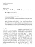
Figure 1: (a) Scheme of a GNSS acquisition block using coherent
integrations only. The low-pass filters after the cosine/sine multi-
plications have been omitted, since the coherent integrations block
already acts like a low-pass filter. (b) Equivalent acquisition scheme
in terms of complex signals.
example, by means of TF techniques. The interference mean
power is defined as the variance of the disturbing signal
I
IF
[n]:
J[n]
= Var{I
IF
[n]},(6)
that can be, in general, time-varying. The jammer-to-noise
ratio is defined as
J[n]
N
=
J[n]
σ

2
IF
=
J[n]
N
0
B
IF
. (7)
As a result of code orthogonality, the different GNSS codes
are analyzed separately by the acquisition block and thus the
case of a single satellite is considered hereinafter; thus the
resulting signal is
r[n]
=

2Cc[n −τ
0
]d[n −τ
0
]cos(2πF
D,0
n + ϕ
0
)
+ I
IF
[n]+W
IF
[n],

(8)
where F
D,0
= ( f
IF
+ f
0
d
)T
s
and τ
0
= τ
a
0
/T
s
.
2.1. The acquisition process
In Figure 1(a), the scheme of a conventional acquisition
system [10] is shown: a local replica of the GNSS code,
delayed by τ, and two orthogonal sinusoids at the frequency
F
D
= ( f
IF
+ f
d
)T
s

are generated and multiplied by the received
signal r[n]. The resulting signals are coherently integrated
leading to the in-phase and quadrature components S
I
(τ, F
D
)
and S
Q
(τ, F
D
). N is the number of samples used for the
integration process and NT
s
is the coherent integration time.
S
I
(τ, F
D
)andS
Q
(τ, F
D
) are then squared and summed,
removing the dependence from the input signal phase ϕ
0
.
In this way, a bidimensional function S(τ, F
D
) is obtained.

S(τ, F
D
) is evaluated for a finite and discrete set of values of τ
and F
D
of the type
τ
= τ
b
+ mΔτ, m = 0,1, , H −1,
(9)
F
D
= F
b
+ lΔ f , l = 0, 1, , K −1.
(10)
The values of the parameters τ
b
, F
b
, Δτ, Δ f , H,andK depend
on various factors, whose analysis is out of the scope of this
paper. The grid of values of τ and F
D
represents the so-called
search space, which is a plane, containing N
t
= H × K cells,
H delay bins, and K Doppler bins.

In Figure 1(b), the traditional acquisition scheme has
been restated in terms of complex signals: the multiplication
by the two orthogonal sinusoids is interpreted as a complex
modulation whereas the sum of the squared in-phase and
quadrature components is represented as a complex square
modulus. In this way, S(τ, F
D
)canbeexpressedas
S(τ, F
D
) =





1
N
N−1

n=0
r[n]c[n −τ]exp{−j2πF
D
n}





2

. (11)
2.2. The spectrogram
The magnitude squared of the Fourier transform is the
classical method used to represent the frequency information
or spectrum of a stationary signal. However, the classical
Fourier transform results completely ineffective when deal-
ing with nonstationary signals, since the time variation of
frequency information is averaged over the whole signal
duration. A solution is represented by the STFT [2, 19]which
is evaluated by applying a suitable windowing function to
the original signal and evaluating the conventional Fourier
transform of the resulting finite length sequence. The STFT
of a finite-length discrete signal r[n]isgivenby
STFT(τ, f )
=
N−1

n=0
r[n]w[n −τ]exp{−j2πfn}, (12)
where w[τ] is the windowing function of duration T
w
.
Although the summation in (12) is performed over the whole
signal duration, the windowing function w[τ]capturesonly
T
w
samples of signal r[n]foreachvalueofτ. r[n]is
assumed stationary over the short time interval T
w
. Using

this technique, an approximation to the spectral content at
the midpoint of the window interval can be achieved by
computing S
w
(τ, f ) =|STFT(τ, f )|
2
that is the discrete spec-
trogram [2, 19]:
S
w
(τ, f ) =





N−1

n=0
r[n]w[n −τ]exp{−j2πfn}





2
. (13)
The TF resolution of the STFT and of the spectrogram
is strictly related to the window length: large T
w

allows a
good frequency resolution at the expense of the time char-
acterization. Conversely, short analysis windows guarantee
better time resolutions. For this reason, different analysis
windows have to be tested in order to provide a good TF
characterization of the signal under analysis [20].
4 EURASIP Journal on Advances in Signal Processing
By comparing (11)and(13), it clearly emerges that the
decision variable for the acquisition block is a spectrogram
scaled by the factor 1/N
2
and with
w[τ]
= c[τ] (14)
that is with the analysis window adapted to the GNSS
signal. Since S(τ, F
D
)andS
w
(τ, f ) have basically the same
structure, the same functional blocks used for evaluating
S(τ, F
D
) can be employed for determining S
w
(τ, f ). Thus,
by replacing the local code with an appropriate analysis
window and by extending the Doppler frequency interval in
order to include all the frequency bands possibly affected
by interfering signals, the acquisition block can be easily

employed for TF applications.
3. THE MODIFIED ACQUISITION BLOCK
In the GNSS literature [9, 18, 21], different acquisition
schemes are employed for determining a first, rough estima-
tion of the code delay and Doppler frequency of the signal
emitted by the satellite under analysis. These methods can be
classified in three main classes:
(i) the classical serial search acquisition scheme [17, 22]
that evaluates the search space cell by cell, subse-
quently testing the different values of code delay and
Doppler shift;
(ii) the frequency domain FFT acquisition scheme [18],
that exploits the fast Fourier transform (FFT) to
evaluate all the Doppler frequencies in parallel. In this
scheme, an integrate and dump (I&D) block can be
used in order to reduce the frequency points to be
evaluated by the FFT. The use of the FFT comports
the analysis of frequency points outside the Doppler
range;
(iii) the time domain FFT acquisition scheme [15], that
uses the FFT to compute fast code circular convolu-
tion.
In this section, those three acquisition schemes are adapted
in order to allow TF frequency applications. As highlighted
in the previous section, the main differences between the
decision variable(11) and the spectrogram (13) consist in fact
of the following:
(i) the set of Doppler frequencies (10), searched for
during the acquisition process, is usually limited to a
few kHz around the receiver intermediate frequency,

whereas the spectrogram needs to be evaluated for a
wider range of frequencies;
(ii) the spectrogram and the decision variable S(τ, F
D
)
employ two different analysis windows.
Thus in order to reuse the acquisition computational re-
sources for TF applications, these two differences have to
be overcome. This can be easily achieved by introducing a
window generator able to produce an analysis window for the
TF analysis. The window generator can be either a memory
bank or a digital device producing signals used as analysis
window. Different analysis windows [16] can be stored in the
memory bank and different window lengths can be obtained
by means of downsampling: in the memory bank the full
length version of an analysis window is stocked; when a
shorter window is needed to increase the spectrogram time
resolution, a new window is produced by downsampling the
original one and adding the corresponding number of zeros.
The simplest digital device producing analysis windows can
be a generator of the signal
w[n]
=
⎧
⎨
⎩
1, for n = 0,1, ,T
w
−1,
0, for n

= T
w
, , N − 1,
(15)
where T
w
and N are the window and the local code length,
respectively. Notice that varying the window length, the
time-frequency resolution changes and different window
lengths can be suitable for different kinds of interference.
The window signal w[n] should have the same length of
the received signal r[n] and of the local code c[n], since the
correlation is usually evaluated by multiplying two signals of
the same length and integrating the result. A selector is used
to switch from the normal acquisition mode to the TF one:
in this way the local code c[n] is substituted by the signal
w[n].
The delay τ, used to progressively shift the window
analysis in (13), can assume values that are not in the set
usually used for the search space computation. In particular,
the step, Δτ, used to explore all possible delay values (9)can
be greater than T
s
, the sampling interval. This allows faster
computations and produces downsampled versions of the
spectrogram that can be used for preliminary analysis.
The frequency range (10) can be extended by changing
the initial frequency F
b
, the frequency step Δ f , and the

number of frequency bins K. This can be achieved by adop-
ting a frequency generator specifically designed for exploring
a wider range of frequencies. The choice of increasing the
number of Doppler bins comports a greater computational
load whereas a too large frequency step Δ f canresultina
spectrogram poorly represented along the frequency dimen-
sion. For this reason, a compromise between frequency
representation and computational load can be reached by
changing both the Doppler step and the number of frequency
bins.
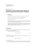
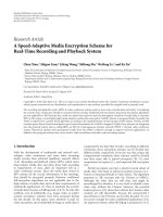
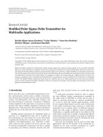
In Figures 2, 3,and4, the traditional acquisition schemes
have been modified, introducing a window generator and an
alternative frequency generator, allowing the evaluation of
the spectrogram. It can be noted that the parallel acquisition
scheme in frequency domain does not require an alternative
frequency generator, since the use of the FFT for exploring
the Doppler dimension already allows to analyze frequency
points outside the Doppler range. In this case, the range of
frequency under analysis depends on L, the number of points
integrated by the I&D block.
4. TIME-FREQUENCY DETECTOR
GNSS acquisition is essentially a detection procedure used
for establishing the presence or the absence of a signal
D. Borio and L. Lo Presti 5
Frequency
generator
Alternative
frequency
generator
Code

generator
Window
generator
r[n]
90
◦
F
D
F

D
τ
τ

1
N
N−1

n=0
(·)(·)
2
1
N
N−1

n=0
(·)
(
·)
2

Figure 2: Modified serial search acquisition. The traditional serial
search acquisition scheme has been modified in order to explore a
wider range of Doppler frequencies and to allow the use of specific
analysis windows for TF applications.
Window
generator
Code
generator
r[n]
L
I&D
ττ

1
L
L−1

n=0
(·)
(
·)
2
Re
FFT
Im
(
·)
2
Figure 3: Modified parallel acquisition in frequency domain. The
parallel acquisition scheme in frequency domain has been modified

allowing the use of specific analysis windows for TF applications.
emitted by a specific satellite. Similarly, one of the main
goals of the modified acquisition schemes proposed in the
previous section is to detect the presence of disturbing
signals. In traditional acquisition, the presence of the useful
signal is declared when the decision statistic (11) passes
a fixed threshold. This threshold is generally chosen in
order to guarantee a certain false alarm probability, that
is the probability that the decision statistic (11)leadstoa
detection when the signal is absent or not correctly aligned,
either in time or in frequency. The proposed algorithm
considers interference in the same way traditional acquisition
schemes consider useful GNSS signals, where the analysis
window is the “local code” that matches the interference TF
characteristics. Thus the interfering signal can be detected
by means of a threshold that is fixed according to the in-
terference false alarm probability that is the probability that
the spectrogram (13) leads to an interference detection in
absence of disturbing signals.
When the interference signal is absent, the input signal
(8)becomes
r[n]
=

2Cc[n −τ
0
]d[n −τ
0
]cos(2πF
D,0

n + ϕ
0
)+W
IF
[n].
(16)
Moreover, the useful GNSS signal when the despreading
process is not correctly performed is generally negligible with
respect to the noise component and thus the signal that
Frequency
generator
Alternative
frequency
generator
Code
generator
Window
generator
r[n]
90
◦
j
F
D
F

D
τ
τ


(·)
∗
(·)
2
(·)
2
Re
IFFTFFT
FFT
Im
Figure 4: Modified parallel acquisition scheme in time domain. The
parallel acquisition scheme in time domain has been modified in
order to explore a wider range of Doppler frequencies and to allow
the use of specific analysis windows for TF applications.
enters the modified acquisition block for TF applications can
be effectively approximated as [9]
r[n]
≈ W
IF
[n]. (17)
In this way, r[n] can by considered as a white Gaussian
process with zero mean and variance σ
2
IF
= N
0
B
IF
. Under this
condition, the STFT (12), for each value of τ and f ,isazero

mean Gaussian process with the variance
Var
{STFT(τ, f )}
=
E{STFT(τ, f )STFT(τ, f )
∗
}
=
N−1

n=0
N
−1

k=0
E

r[n]w[n−τ]r[k]w
∗
[k−τ]exp{−j2πf(n−k)}

=
N−1

n=0
E{W
2
IF
[n]}|w[n −τ]|
2

= σ
2
IF
N
−1

n=0
|w[n −τ]|
2
= E
w
σ
2
IF
,
(18)
where E
w
is the analysis window energy, that is independent
from the delay applied to w[n].
Furthermore, it is possible to show [23] that the square
absolute value of a zero mean complex Gaussian random
variable is a new random variable distributed according to
an exponential law. More specifically, it is
S
w
(τ, f )∼Exp

1
σ

2
out

, (19)
where σ
2
out
= E
w
σ
2
IF
is the variance of STFT(τ, f ). The pro-
bability density function of S
w
(τ, f ) results in
f
w
(s) =
1
σ
2
out
exp

−
s
σ
2
out


(20)
and finally the interference false alarm probability equals
P
fa,I
(β) =

+∞
β
f
w
(s)ds = exp

−
β
σ
2
out

, (21)
6 EURASIP Journal on Advances in Signal Processing
Table 1: NordNav-R30 characteristics.
Sampling frequency f
s
= 16.3676 MHz
Intermediate frequency f
s
= 4.1304 MHz
Signal quantization 4 bits
Front-end filter bandwidth

≈ 2MHz
where β is the threshold to be determined by fixing the
false alarm probability and inverting (21). In this way, the
threshold formula results in
β
=−σ
2
out
log P
fa, I
. (22)
It has to be noted that when the modified acquisition process
is used for evaluating the spectrogram, then (13) is scaled by
afactor1/N
2
, thus the threshold (22) has to be scaled by the
same factor:
β

=−
E
w
σ
2
IF
N
2
log P
fa, I
. (23)

Equation (23) is very close to the expression for the threshold
for the traditional acquisition, and thus the same structures
used for the satellite detection can be directly used for the
interfering monitoring.
5. REAL-DATA AND SIMULATION TEST
Inordertoprovetheeffectiveness of the proposed acqui-
sition scheme, some examples based on simulated and real
data are reported in this section.
5.1. Real data
Real data have been collected by using the NordNav-R30
front-end [24] that is characterized by the specifications
reported in Tabl e 1 . Data collection has been extensively
performed in two different sites: the so-called “colle della
Maddalena” and the hill of the “Basilica di Superga”. These
sites are located on two different hills on the side of Torino
(Italy). The first one is characterized by the presence of
several antennas for the transmission of analog and digital
TV signals, whereas the second one is in direct view of
the colle della Maddalena antennas. Two different kinds of
interference have been observed. In the proximity of the colle
della Maddalena, the GPS signal was corrupted by a swept
interference, whereas a strong continuous wave interference
(CWI) has been observed on the hill of Superga.
In Figure 5, the spectrogram of the swept interference
observed in proximity of the colle della Maddalena has been
depicted. This spectrogram has been evaluated by employing
the modified parallel acquisition scheme in time domain
described in the previous section. The input signal has been,
at first, downsampled by a factor of 4 reducing the sampling
frequency to f

s
= 4.0919 MHz. This operation reduces the
computational load without effectively degrading the signal
quality since the NordNav front-end is characterized by a
bandwidth of about 2 MHz. The Doppler step has been set
to 10 kHz and the number of Doppler bins was K
= 201.
0
2
4
6
8
×10
−5
2
1.5
1
0.5
0
(MHz)
0
2
4
6
8
10
(ms)
Figure 5: Spectrogram of a swept interference. The input signal
has been collected by using the NordNav R30 front-end in the
proximity of TV repeaters in Torino (Italy). The spectrogram has

been evaluated by using the modified parallel acquisition scheme in
time domain.
−90
−80
−70
−60
−50
−40
Power/frequency
(dB/Hz)
012345678
Frequency (MHz)
Swept interference
(a) Welch power spectral density estimate—original signal
−65
−60
−55
−50
−45
Power/frequency
(dB/Hz)
00.20.40.60.811.21.41.61.820
Frequency (MHz)
Swept interference
(b) Welch power spectral density estimate—downsampled signal
Figure 6: Power spectral density estimates of the input signal used
for the evaluation of the spectrogram in Figure 5.(a)PSDofthe
original signal, sampling frequency f
s
= 16.3676 MHz. (b) PSD of

the downsampled signal, sampling frequency f
s
= 4.0919 MHz.
A Hamming window of duration T
w
= N/10 was employed.
The analysis was extended to a signal portion of 10 millisec-
onds. The presence of the swept interference clearly emerges
from Figure 5, that can be easily used for the estimation of
the interference instantaneous frequency. The information
extracted from the spectrogram in Figure 5 can then be easily
used for different excision algorithms [4, 7]. In Figure 6,
the power spectral density (PSD) of the input signal has
been reported. In Figure 6(a), the PSD has been estimated by
considering the downconverted GPS signal with a sampling
D. Borio and L. Lo Presti 7
0
0.2
0.4
0.6
0.8
1
1.2
1.4
1.6
1.8
×10
−3
2.5
2

1.5
0.5
1
0
(MHz)
0
0.2
0.4
0.6
0.8
1
(ms)
Figure 7: Spectrogram of a CWI. The input signal has been col-
lected by using the NordNav R30 front-end on the hill of Superga,
Torino (Italy). The spectrogram has been evaluated by using the
modified parallel acquisition scheme in time domain.
frequency f
s
= 16.3676 MHz: in this case the interference
spectral components clearly emerge, although they are
spread over a band of more than 1 MHz. Downsampling
makes the PSD of the input signal fold, producing a noise
term that is almost white and aliasing the interfering signal
at a different frequency. The presence of a white noise term
makes a wideband interfering signal hardly detectable in
the frequency domain. In Figure 6(b), the PSD of the signal
used for the evaluation of the spectrogram in Figure 5 has
been depicted. In this case, the interference cannot be easily
localized in the frequency domain, proving the effectiveness
of TF detection techniques versus traditional pure frequency

detection methods.
In Figures 7 and 8, the spectrogram and the PSDs of the
signal observed at the hill of Superga are depicted. In this
case, the CWI is well localized in both TF and frequency
domains. The spectrogram has been evaluated by using the
modified parallel acquisition scheme in time domain, with
a Hamming window of duration T
w
= N/8. As for the first
case, the Doppler step has been set to 10 kHz and the number
of Doppler bins was K
= 201.
5.2. Simulated data
In order to further test the modified acquisition scheme for
TF interference detection, the case of pulsed interference has
been considered. In particular, GPS signals in presence of
pulsed interference have been simulated and analyzed with
the modified parallel acquisition scheme in time domain.
The same sampling frequency and intermediate frequency
of Tab le 1 have been adopted for the simulation. Pulsed
interference can be generated by different sources such as
distance measuring equipment (DME) and tactical airborne
navigation (TACAN) [25] that are currently used for distance
measuring and for civil and military airborne landing. The
pulsed interference has been simulated as a pair of modulated
Gaussian impulses [25]. The results of the test have been
depicted in Figure 9, where the case of impulses with a peak
−85
−80
−75

−70
−65
−60
−55
−50
Power/frequency
(dB/Hz)
012345678
Frequency (MHz)
CWI
(a) Welch power spectral density estimate—original signal
−65
−60
−55
−50
−45
−40
Power/frequency
(dB/Hz)
00.20.40.60.811.21.41.61.820
Frequency (MHz)
CWI
(b) Welch power spectral density estimate—downsampled signal
Figure 8: Power spectral density estimates of the input signal used
for the evaluation of the spectrogram in Figure 7.(a)PSDofthe
original signal, sampling frequency f
s
= 16.3676 MHz. (b) PSD of
the downsampled signal, sampling frequency f
s

= 4.0919 MHz.
0
1
2
3
4
×10
−5
1
0.8
0.6
0.4
0.2
(ms)
8
6
4
2
0
(MHz)
(a)
−10
−5
0
5
0.10.20.30.40.50.60.70.80.91
ms
(b)
Figure 9: Spectrogram and time domain representation of a simu-
lated GPS signal corrupted by pulsed interference. The spectrogram

has been evaluated by using the modified parallel acquisition
scheme in time domain.
power equal to the noise variance has been considered. In
the bottom part of Figure 9, the time representation of the
input signal has been depicted. The light line represents the
envelope of the pulsed interference that cannot be directly
identified from the time representation of the input signal.
8 EURASIP Journal on Advances in Signal Processing
When the TF representation is considered, the pulsed inter-
ference is clearly identified, allowing the efficient excision of
the disturbing signal. The spectrogram of Figure 9 has been
evaluated by using the modified parallel acquisition scheme
in time domain, with a Hamming window of duration T
w
=
N/64. The Doppler step has been set to 200 kHz and the
number of Doppler bins was K
= 41.
6. CONCLUSIONS
In this paper, the problem of effectively implementing TF
algorithms in GNSS receivers has been addressed. More
specifically, a modified acquisition algorithm has been pro-
posed in order to efficiently reuse the hardware already
available in a GNSS receiver for TF applications. The pro-
posed method is suitable for all acquisition schemes and its
effectiveness has been proven by means of analysis on real
data and by simulations.
ACKNOWLEDGMENTS
The authors would like to thank Laura Camoriano and
Tereza Cristina Gondim Corsini for their support during

data collection.
REFERENCES
[1] R. J. Landry and A. Renard, “Analysis of potential interference
sources and assessment of present solutions for GPS/GNSS
receivers,” in Proceedings of the 4th Saint Petersburg Interna-
tional Conference on Integrated Navigation Systems (INS ’97),
Saint Petersburg, Russia, May 1997.
[2] L. Cohen, Time Frequency Analysis: Theory and Applications,
Prentice Hall PTR, Englewood Cliffs, NJ, USA, 1994.
[3] M. V. Tazebay and A. N. Akansu, “A performance analysis
of interference excision techniques in direct sequence spread
spectrum communications,” IEEE Transactions on Signal Pro-
cessing, vol. 46, no. 9, pp. 2530–2535, 1998.
[4] C. Wang and M. G. Amin, “Performance analysis of instan-
taneous frequency-based interference excision techniques in
spread spectrum communications,” IEEE Transactions on Sig-
nal Processing, vol. 46, no. 1, pp. 70–82, 1998.
[5] M. G. Amin, C. Wang, and A. R. Lindsey, “Optimum inter-
ference excision in spread spectrum communications using
open-loop adaptive filters,” IEEE Transactions on Signal Pro-
cessing, vol. 47, no. 7, pp. 1966–1976, 1999.
[6] X. Ouyang and M. G. Amin, “Short-time Fourier transform
receiver for nonstationary interference excision in direct
sequence spread spectrum communications,” IEEE Transac-
tions on Signal Processing, vol. 49, no. 4, pp. 851–863, 2001.
[7] S. Barbarossa and A. Scaglione, “Adaptive time-varying can-
cellation of wideband interferences in spread-spectrum com-
munications based on time-frequency distributions,” IEEE
Transactions on Signal Processing, vol. 47, no. 4, pp. 957–965,
1999.

[8] S. R. Lach, M. G. Amin, and A. R. Lindsey, “Broadband inter-
ference excision for software-radio spread-spectrum commu-
nications using time-frequency distribution synthesis,” IEEE
Journal on Selected Areas in Communications, vol. 17, no. 4,
pp. 704–714, 1999.
[9] E.D.KaplanandC.Hegarty,Eds.,Understanding GPS: Princ i-
ples and Applications, Artech House, Boston, Mass, USA, 2nd
edition, 2005.
[1 0 ] P. M i sr a a n d P. E n g e , Global Positioning System, Signals, Mea-
surements and Performance, Ganga-Jamuna Press, Lincoln,
Mass, USA, 2006.
[11] R. J. Landry, V. Calmettes, and M. Bousquet, “Impact of
interference on a generic GPS receiver and assessment of miti-
gation techniques,” in Proceedings of the 5th IEEE International
Symposium on Spread Spectrum Techniques and Applications
(ISSSTA ’98), vol. 1, pp. 87–91, Sun City, South Africa, Sep-
tember 1998.
[12] J. A. Young and J. S. Lehnert, “Analysis of DFT-based fre-
quency excision algorithms for direct-sequence spread-spec-
trum communications,” IEEE Transactions on Communica-
tions, vol. 46, no. 8, pp. 1076–1087, 1998.
[13] Z. Yimin, M. G. Amin, and A. R. Lindsey, “Anti-jamming
GPS receivers based on bilinear signal distributions,” in
Proceedings of the IEEE Military Communications Conference
(MILCOM ’01), vol. 2, pp. 1070–1074, McLean, Va, USA,
October 2001.
[14] C. Yang, “Method and device for rapidly extracting time and
frequency parameters from high dynamic direct sequence
spread spectrum radio signals under interference,” US patent
6407699, June 2002.

[15] D. J. R. van Nee and A. J. R. M. Coenen, “New fast GPS code-
acquisition technique using FFT,” Electronics Letters, vol. 27,
no. 2, pp. 158–160, 1991.
[16] F. J. Harris, “On the use of windows for harmonic analysis with
the discrete Fourier transform,” Proceedings of the IEEE, vol.
66, no. 1, pp. 51–83, 1978.
[17] Z. Weihua and J. Tranquilla, “Modeling and analysis for the
GPS pseudo-range observable,” IEEE Transactions on Aer-
ospace and Electronic Systems, vol. 31, no. 2, pp. 739–751, 1995.
[18] J. B Y. Tsui, Fundamentals of Global Positioning System
Receivers: A Software Approach, Wiley-Interscience, New York,
NY, USA, 2000.
[19] F. Hlawatsch and G. F. Boudreaux-Bartels, “Linear and qua-
dratic time-frequency signal representations,”
IEEE Signal
Processing Magazine, vol. 9, no. 2, pp. 21–67, 1992.
[20] M. G. Amin and K. Di Feng, “Short-time Fourier transforms
using cascade filter structures,” IEEE Transactions on Circuits
and Systems II, vol. 42, no. 10, pp. 631–641, 1995.
[21] D. Akopian, “Fast FFT based GPS satellite acquisition meth-
ods,” IEE Proceedings: Radar, Sonar and Navigation, vol. 152,
no. 4, pp. 277–286, 2005.
[2 2 ] P. M i sr a a n d P. E n g e , Global Positioning System: Signals, Mea-
surements and Performance, Ganga-Jamuna Press, Lincoln,
Mass, USA, 2006.
[23] J. Proakis, Digital Communications, McGraw-Hill, New York,
NY, USA, 4th edition, 2000.
[24] NordNav-R30 Package, NordNav Technologies, 2004, http://
www.navtechgps.com/pdf/r30.pdf.
[25] F. Bastide, E. Chatre, C. Macabiau, and B. Roturier, “GPS L5

and Galileo E5a/E5b signal-to-noise density ratio degradation
due to DME/TACAN signals: simulations and theoretical
derivation,” in Proceedings of the ION/NTM National Technical
Meeting, pp. 1049–1062, San Diego, Calif, USA, January 2004.