Báo cáo hóa học: " Research Article Coorbit Theory, Multi-α-Modulation Frames, and the Concept of Joint Sparsity for Medical " ppt

Hindawi Publishing Corporation
EURASIP Journal on Advances in Signal Processing
Volume 2008, Article ID 471601, 19 pages
doi:10.1155/2008/471601
Research Article
Coorbit Theory, Multi-α-Modulation Frames, and the Concept
of Joint Sparsity for Medical Multichannel Data Analysis
Stephan Dahlke,
1
Gerd Teschke,
2, 3
and Krunoslav Stingl
4
1
FB 12 - Faculty of Mathematics and Computer Sciences, Philipps-University of Marburg, Hans-Meerwein-Street,
Lahnberge, 35032 Marburg, Germany
2
Institute for Computational Mathematics in Science and Technology, University of Applied Sciences Neubrandenburg,
Brodaer Street 2, 17033 Neubrandenburg, Germany
3
Zuse Institute Berlin, Takustrasse 7, 14195 Berlin-Dahlem, Germany
4
MEG-Center T
¨
ubingen, Otfried M
¨
uller Strasse 47, 72076 T
¨
ubingen, Germany
Correspondence should be addressed to Gerd Teschke,
Received 30 November 2007; Revised 8 August 2008; Accepted 19 August 2008

Recommended by Qi Tian
This paper is concerned with the analysis and decomposition of medical multichannel data. We present a signal processing
technique that reliably detects and separates signal components such as mMCG, fMCG, or MMG by involving the spatiotemporal
morphology of the data provided by the multisensor geometry of the so-called multichannel superconducting quantum
interference device (SQUID) system. The mathematical building blocks are coorbit theory, multi-α-modulation frames, and the
concept of joint sparsity measures. Combining the ingredients, we end up with an iterative procedure (with component-dependent
projection operations) that delivers the individual signal components.
Copyright © 2008 Stephan Dahlke et al. This is an open access article distributed under the Creative Commons Attribution
License, which permits unrestricted use, distribution, and reproduction in any medium, provided the original work is properly
cited.
1. INTRODUCTION
One focus in the field of prenatal diagnostics is the
investigation of fetal developmental brain processes that
are limited by the inaccessibility of the fetus. Currently,
there exist two techniques for the study of fetal brain
function in utero, namely, functional magnetic resonance
imaging (fMRI) [1, 2] and fetal magnetoencephalography
(fMEG) [3–6]. There are several advantages and disad-
vantages of both techniques. The fMEG, for instance,
is a completely passive and noninvasive method with
superior temporal resolution and is currently measured
by a multichannel superconducting quantum interference
device (SQUID) system, see Figure 1.However,thefMEG
is measured in the presence of environmental noise and
various near-field biological signals and other interference
as, for example, maternal magnetocardiogram (mMCG),
fetal magnetocardiogram (fMCG), uterine smooth muscle
(magnetomyogram
= MMG), and motion artifacts [7, 8].
After the removal of environmental noise [9], the emphasis

is on the detection and separation of mMCG, fMCG, and
MMG. Solving this detection problem seriously is the main
prerequisite for observing and analyzing the fMEG. In the
majority of reported work, the MCG was reduced by adaptive
filtering and/or noise estimation techniques [10, 11]. In [10],
different algorithms for elimination of MCG from MEG
recordings are considered, for example, direct subtraction
(DS) of an MCG signal, adaptive interference cancellation
(AIC), and orthogonal signal projection algorithms (OSPAs).
All these approaches and their slightly modified versions
are used for fMEG detection. In this paper, we present a
different data processing technique that reliably detects both
the mMCG + fMCG and MMG + “motion artifacts” by
involving the spatiotemporal morphology of the data given
by the multisensor geometry information. Mathematically,
the main ingredients of our procedure are the so-called
multi-α-modulation f rames (for which the construction relies
on the theory of coorbit spaces) for an optimal/sparse
signal expansion and the concept of joint sparsity mea-
sures.
A sparse representation of an element in a Hilbert or
Banach space is a series expansion with respect to an
2 EURASIP Journal on Advances in Signal Processing
Figure 1: Multichannel superconducting quantum interference
device (SQUID) system.
orthonormal basis or a frame that has only a small number of
large/nonzero coefficients. Several types of signals appearing
in nature admit sparse frame expansions, and thus sparsity
is a realistic assumption for a very large class of problems.
Recent developments have shown the practical impact of

sparse signal reconstruction (even the possibility to recon-
struct sparse signals from incomplete information [12–14]).
This is in particular the case for the medical multichannel
data under consideration that usually consist of pattern
representing specific biomedical information (mMCG and
fMCG). But multichannel signals (i.e., vector valued func-
tions) may not only possess sparse frame expansions for
each channel individually, but additionally (and this is the
novelty) the different channels can also exhibit common
sparsity patterns. The mMCG and fMCG exhibit a very
rich morphology that appears in all the channels at the
same temporal locations. This will be reflected, for example,
in sparse wavelet/Gabor expansions [15, 16]withrelevant
coefficients appearing at the same labels, or in turn in sparse
gradients with supports at the same locations. Hence, an
adequate sparsity constraint is the so-called common or joint
sparsity measure that promotes patterns of multichannel
data that do not belong only to one individual channel but
to all of them simultaneously.
In order to sparsely represent the MCG data, we propose
the usage of multi-α-modulation frames. These frames have
only been recently developed as a mixture of Gabor and
wavelet frames. Wavelet frames are optimal for piecewise
smooth signals with isolated singularities, whereas Gabor
frames have been very successfully applied to the analysis
of periodic structures. Therefore, the α-modulation frames
have the potential to detect both features at the same time,
so they seem to be extremely well suited for the problems
studied in this paper. Indeed, the numerical experiments
presented here definitely confirm this conjecture.

This paper is organized as follows. In Section 2,webriefly
recall the setting of α-modulation frames as far as this is
needed for our purposes. Then, in Section 3, we explain how
these frames can be used in multichannel data processing
involving joint sparsity constraints. Finally, in Section 4,we
present the numerical experiments.
2. COORBIT THEORY AND α-MODULATION FRAMES
In this section, we review the basic that provides the so-
called α-modulation frames. We propose to treat the medical
data analysis problem with this specific kind of frame
expansions since varying the parameter α allows to switch
between completely different frame expansions highlighting
different features of the signal to be analyzed while having
to manage only one frame construction principle. The focus
is not yet on multichannel data approximation but rather
on the basic methodologies that apply for single-channel
signals but can simply be extended to multichannel data (in
Section 3).
In general, the motivation (and central issue in applied
analysis) is the problem of analyzing and approximating
a given signal. The first step is always to decompose the
signal with respect to a suitable set of building blocks.
These building blocks may, for example, consist of the
elements of a basis, a frame, or even of the elements of
huge dictionaries. Classical examples with many important
practical applications are wavelet bases/frames and Gabor
frames, respectively. The wavelet transform is very useful to
analyze piecewise smooth signals with isolated singularities,
whereas the Gabor transform is well-suited for the analysis
of periodic structures such as textures. Quite surprisingly,

there is a common thread behind both transforms, and that
is a group theory. In general, a unitary representation U of a
locally compact group G in a Hilbert space H is called square
integrable if there exists a function ψ
∈ H such that

G



ψ, U(g)ψ
H


2
dμ(g) < ∞,(1)
where dμ denotes the (left) Haar measure on G. In this case,
the voice transform
V
ψ
f (g):=f , U(g)ψ
H
(2)
is well defined and invertible on its range by its adjoint. It
turns out that the Gabor transform can be interpreted as the
voice transform associated with a representation of the Weyl-
Heisenberg group in L
2
, whereas the wavelet transform is
related with a square-integrable representation of the affine

group in L
2
.
Since both transforms have their specific advantages, it is
quite natural to try to combine them in a joint transform.
Stephan Dahlke et al. 3
−2000
−1500
−1000
−500
0
500
1000
1500
2000
45216 2000
2608.3 6441.2
simulation
real
s1
s2
ampli freq
power
centre
2000 7 1 42 RUN
0.6
ZOOM
−15
−10
−5

0
5
10
15
20
25
30
Z axis
−20 −15 −10 −50 5 1015
Y axis
−2000
−1500
−1000
−500
0
500
1000
1500
2000
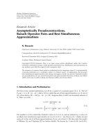
Figure 2: Left: second component, generated by combination of two sinusoidal functions (7 Hz and 0.6 Hz). The different amplitudes
correspond to signals of the different channels. Right: geometric visualization of the SQUID device with 151 sensors (coils). The color
encodes the Gaussian weighting, that is, the influence of the synthetic background signal. The center of appearance of the synthetic signal is
marked by a circle.
One way to achieve this would be to use the affine Weyl-
Heisenberg group G
aWH
which is the set R
2+1
× R
+

equipped
with group law
(q, p, a, ϕ)
◦

q

, p

, a

, ϕ


=

q + aq

, p + a
−1
p

, aa

, ϕ + ϕ

+ paq


.

(3)
This group has the Stone-Von-Neumann representation on
L
2
(R) as follows:
U(q, p, a, ϕ) f (x)
= a
−1/2
e
2πi(p(x−q)+ϕ)
f

x − q
a

=
e
2πiϕ
T
x
M
ω
D
a
f (t),
(4)
where
M
ω
f (t) = e

2πiωt
f (t), T
x
f (t) = f (t − x),
D
a
f (t) =|a|
−1/2
f

t
a

,
(5)
which obviously contains all three basic operations, that is,
dilations, modulations, and translations. Unfortunately, U is
not square integrable. One way to overcome this problem is
to work with representations modulo quotients. In general,
given a locally compact group G with closed subgroup H,
we consider the quotient group X
= G/H and fix a section
σ : X
→ G. Then, we define the generalized voice transform
V
ψ
f (x):=f , U(σ(x))ψ
H
. (6)
In the case of the affine Weyl-Heisenberg group, it has

been shown in [17] that by using the specific group H :
=
{
(0, 0, a, ϕ) ∈ G
aWH
} and the specific section σ(x, ω) =
(x,ω,β(x, ω), 0), β(x, ω) = (1 + |ω|)
−α
, α ∈ [0, 1), the
associated voice transform (6) is indeed well defined and
invertible on its range. Hence, it gives rise to a mixed form
of the wavelet and the Gabor transform, and it also provides
some kind of homotopy between both cases. Indeed, for
α
= 0, we are in the classical Gabor setting, whereas the case
α
= 1 is very close to the wavelet setting (see, e.g., [17]for
details).
Once a square-integrable representation modulo quo-
tient is established, there is also a natural way to define
associated smoothness spaces, the so-called coorbit spaces,
by collecting all functions for which the voice transform
has a certain decay, see [18–20]. More precisely, given some
positive measurable weight function v on X and 1
≤ p ≤∞,
let
L
p,v
(X):=


f measurable : fv∈ L
p
(X)

. (7)
Then, for suitable ψ, we define the spaces
H
p,v
:=

f : V
ψ

A
−1
σ
f

∈ L
p,v

,
A
σ
f :=

X

f , U(σ(x))ψ


H
U(σ(x))ψdμ,
(8)
where dμ denotes a quasi-invariant measure on X. In the
classical cases, that is, for the affine group and the Weyl-
Heisenberg group, one obtains the Besov spaces and the
modulation spaces, respectively. In the setting of the affine
Weyl-Heisenberg group and the specific case v
s
(ω) = (1 +
|ω|)
s
, the following theorem has been shown in [17].
4 EURASIP Journal on Advances in Signal Processing
Channel: 1 (data)
−800
−600
−400
−200
0
200
400
600
200 400 600 800 1000
Channel: 2 (data)
−6000
−5000
−4000
−3000
−2000

−1000
0
1000
200 400 600 800 1000
Channel: 1 (data)
−500
−400
−300
−200
−100
0
100
200
300
400
200 400 600 800 1000
Channel: 2 (data)
−6000
−5000
−4000
−3000
−2000
−1000
0
1000
200 400 600 800 1000
Channel: 1 (data)
−6000
−5000
−4000

−3000
−2000
−1000
0
1000
200 400 600 800 1000
Channel: 2 (data)
−5000
−4000
−3000
−2000
−1000
0
1000
200 400 600 800 1000
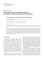
Figure 3: Measured spontaneous activity of selected individual channels. Top row: channel 1 corresponds to coil number 20, and channel 2
corresponds to coil number 40. Middle row: channel 1 corresponds to coil number 80, and channel 2 corresponds to coil number 40. Bottom
row: channel 1 corresponds to coil number 40, and channel 2 corresponds to coil number 41. It can be clearly observed that the neighboring
channels have similar structures, whereas channels with large geometric distance have completely different structures.
Stephan Dahlke et al. 5
Channel: 1 (data)
−1000
−500
0
500
1000
200 400 600 800 1000
Channel: 2 (data)
−1500
−1000

−500
0
500
1000
1500
200 400 600 800 1000
Channel: 1 (data)
−250
−200
−150
−100
−50
0
50
100
150
200
250
200 400 600 800 1000
Channel: 2 (data)
−1500
−1000
−500
0
500
1000
1500
200 400 600 800 1000
Channel: 1 (data)
−1500

−1000
−500
0
500
1000
1500
200 400 600 800 1000
Channel: 2 (data)
−1000
−500
0
500
1000
200 400 600 800 1000
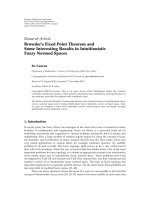
Figure 4: Synthetic sinusoidal signals of selected individual channels. Top row: channel 1 corresponds to coil number 20, and channel
2 corresponds to coil number 40. Middle row: channel 1 corresponds to coil number 80, and channel 2 corresponds to coil number 40.
Bottom row: channel 1 corresponds to coil number 40, and channel 2 corresponds to coil number 41. Due to the Gaussian weighting,
the neighboring channels have similar amplitudes, whereas channels with large geometric distance have significantly different amplitudes
(attenuation).
6 EURASIP Journal on Advances in Signal Processing
0 1000 2000 3000 4000 5000 6000 7000 8000 9000 10000
−2
0
2
0 1000 2000 3000 4000 5000 6000 7000 8000 9000 10000
−
10
0
10
0 1000 2000 3000 4000 5000 6000 7000 8000 9000 10000

−
10
0
10
0 1000 2000 3000 4000 5000 6000 7000 8000 9000 10000
−
5
0
5
0 1000 2000 3000 4000 5000 6000 7000 8000 9000 10000
−
20
0
20
0 1000 2000 3000 4000 5000 6000 7000 8000 9000 10000
−
5
0
5
0 1000 2000 3000 4000 5000 6000 7000 8000 9000 10000
−
5
0
5
0 1000 2000 3000 4000 5000 6000 7000 8000 9000 10000
−
10
0
10
0 1000 2000 3000 4000 5000 6000 7000 8000 9000 10000

−
10
0
10
0 1000 2000 3000 4000 5000 6000 7000 8000 9000 10000
−
5
0
5
0 1000 2000 3000 4000 5000 6000 7000 8000 9000 10000
−
10
0
10
0 1000 2000 3000 4000 5000 6000 7000 8000 9000 10000
−10
0
10
0 1000 2000 3000 4000 5000 6000 7000 8000 9000 10000
−5
0
5
0 1000 2000 3000 4000 5000 6000 7000 8000 9000 10000
−5
0
5
×10
4
Figure 5: Top row: signal to be analyzed. Second to bottom row: ICA decomposition of generated signal “spontaneous activity + sinusoidal
signal,” where the maximum amplitude of the synthetic signal component is 125 fT.

Theorem 1. Let 1 ≤ p ≤∞,0≤ α<1,ands ∈ R.Let
ψ
∈ L
2
w ith supp

ψ compact and

ψ ∈ C
2
. Then the coorbit
spaces H
p,v
s−α(1/p−1/2)
,α
are well defined and can be identified with
the α-modulation spaces M
s,α
p,p
, which are defined by
M
s+α(1/q−1/2),α
p,p
(R)=

f ∈S

(R):

f , U(σ(x, ω))ψ


∈
L
p·v
s
(R
2
)

.
(9)
Consequently, the α-modulation spaces are the natural
smoothness spaces associated with representations modulo
quotients of the affine Weyl-Heisenberg group.
When it comes to practical applications, then one can
only work with discrete data, and therefore it is necessary
to discretize the underlying representation in a suitable
way. Indeed, in a series of papers [18–20], Feichtinger and
Gr
¨
ochenig have shown that a judicious discretization gives
rise to frame decompositions. The general setting can be
described as follows. Given a Hilbert space H , a countable
set
{f
n
: n ∈ N} is called a frame for H if
f 
2
H

∼

n∈N
|f , f
n

H
|
2
∀f ∈ H. (10)
Stephan Dahlke et al. 7
0 1000 2000 3000 4000 5000 6000 7000 8000 9000 10000
0
2
2
0 1000 2000 3000 4000 5000 6000 7000 8000 9000 10000
−10
0
10
0 1000 2000 3000 4000 5000 6000 7000 8000 9000 10000
−10
0
10
0 1000 2000 3000 4000 5000 6000 7000 8000 9000 10000
−5
0
5
0 1000 2000 3000 4000 5000 6000 7000 8000 9000 10000
−5
0

5
0 1000 2000 3000 4000 5000 6000 7000 8000 9000 10000
−20
0
20
0 1000 2000 3000 4000 5000 6000 7000 8000 9000 10000
−10
0
10
0 1000 2000 3000 4000 5000 6000 7000 8000 9000 10000
−5
0
5
0 1000 2000 3000 4000 5000 6000 7000 8000 9000 10000
−5
0
5
0 1000 2000 3000 4000 5000 6000 7000 8000 9000 10000
−
10
0
10
0 1000 2000 3000 4000 5000 6000 7000 8000 9000 10000
−10
0
10
0 1000 2000 3000 4000 5000 6000 7000 8000 9000 10000
−10
0
10

0 1000 2000 3000 4000 5000 6000 7000 8000 9000 10000
−5
0
5
0
1000 2000 3000 4000 5000 6000 7000 8000 9000 10000
−5
0
5
−
×10
4
Figure 6: Top row: signal to be analyzed. Second to bottom row: ICA decomposition of generated signal “spontaneous activity + sinusoidal
signal,” where the maximum amplitude of the synthetic signal component is 250 fT.
As a consequence of (10), the corresponding operators of
analysis and synthesis given by
F : H
−→ 
2
(N), f −→

f , f
n

H

n∈N
, (11)
F
∗

: 
2
−→ H , c −→

n∈N
c
n
f
n
(12)
are bounded. The composition S :
= F
∗
F is boundedly
invertible and gives rise to the following decomposition and
reconstruction formulas:
f
= SS
−1
f =

n∈N

f , S
−1
f
n

H
f

n
= S
−1
Sf =

n∈N
f , f
n

H
S
−1
f
n
.
(13)
The Feichtinger-Gr
¨
ochenig theory gives rise to frame decom-
positions of this type, not only for the underlying represen-
tation space H but also for the associated coorbit spaces.
Indeed, it is possible to decompose any element in the
8 EURASIP Journal on Advances in Signal Processing
0 1000 2000 3000 4000 5000 6000 7000 8000 9000 10000
0
2
2
0 1000 2000 3000 4000 5000 6000 7000 8000 9000 10000
−
−

10
0
10
0 1000 2000 3000 4000 5000 6000 7000 8000 9000 10000
−5
0
5
0 1000 2000 3000 4000 5000 6000 7000 8000 9000 10000
−10
0
10
0 1000 2000 3000 4000 5000 6000 7000 8000 9000 10000
−5
0
5
0 1000 2000 3000 4000 5000 6000 7000 8000 9000 10000
−20
0
20
0 1000 2000 3000 4000 5000 6000 7000 8000 9000 10000
−5
0
5
0 1000 2000 3000 4000 5000 6000 7000 8000 9000 10000
−5
0
5
0 1000 2000 3000 4000 5000 6000 7000 8000 9000 10000
−10
0

10
0 1000 2000 3000 4000 5000 6000 7000 8000 9000 10000
−5
0
5
0 1000 2000 3000 4000 5000 6000 7000 8000 9000 10000
−5
0
5
0 1000 2000 3000 4000 5000 6000 7000 8000 9000 10000
−10
0
10
0 1000 2000 3000 4000 5000 6000 7000 8000 9000 10000
−10
0
10
0 1000 2000 3000 4000 5000 6000 7000 8000 9000 10000
−5
0
5
×10
4
Figure 7: Top row: signal to be analyzed. Second to bottom row: ICA decomposition of generated signal “spontaneous activity + sinusoidal
signal,” where the maximum amplitude of the synthetic signal component is 500 fT.
coorbit space with respect to the frame elements (atomic
decomposition), and it is also possible to reconstruct it from
its sequence of moments. For the case of the α-modulation
spaces, these results can be summarized as follows.
Theorem 2. Let 1

≤ p ≤∞,0≤ α<1 and s ∈ R.Letψ ∈ L
2
w ith supp

ψ compact and

ψ ∈ C
2
. Then there exists ε
0
> 0 with
the following property. Let Λ(α):
={(x
j,k
, ω
j
)}
j,k∈Z
denote the
point set ω
j
:= p
α
(ε
j
), x
j,k
:= εβ(ω
j
)k,0<ε≤ ε

0
,where
p
α
(ω):= sgn(ω)

(1 + (1 −α)|ω|)
1/(1−α)
−1

, (14)
then the following holds true.
(i) (Atomic decomposition) Any f
∈ M
s,α
p,p
can be written
as
f
=

(j,k)∈Z
2
c
j,k
( f )T
x
j,k
M
ω

j
D
β
α
(ω
j
)
ψ, (15)
and there exist constants 0 <C
1
, C
2
< ∞ (independent of p)
such that
C
1
f 
M
s,α
p,p
≤


(j,k)∈Z
2
|c
j,k
( f )|
p
(1 + (1 −α)|j|)

((s−α(1/p−1/2))/(1−α))p

1/p
≤ C
2
f 
M
s,α
p,p
.
(16)
Stephan Dahlke et al. 9
0 1000 2000 3000 4000 5000 6000 7000 8000 9000 10000
0
2
2
0 1000 2000 3000 4000 5000 6000 7000 8000 9000 10000
−
−
10
0
10
0 1000 2000 3000 4000 5000 6000 7000 8000 9000 10000
−5
0
5
0 1000 2000 3000 4000 5000 6000 7000 8000 9000 10000
−10
0
10

0 1000 2000 3000 4000 5000 6000 7000 8000 9000 10000
−5
0
5
0 1000 2000 3000 4000 5000 6000 7000 8000 9000 10000
−20
0
20
0 1000 2000 3000 4000 5000 6000 7000 8000 9000 10000
−5
0
5
0 1000 2000 3000 4000 5000 6000 7000 8000 9000 10000
−5
0
5
0 1000 2000 3000 4000 5000 6000 7000 8000 9000 10000
−5
0
5
0 1000 2000 3000 4000 5000 6000 7000 8000 9000 10000
−10
0
10
0 1000 2000 3000 4000 5000 6000 7000 8000 9000 10000
−5
0
5
0 1000 2000 3000 4000 5000 6000 7000 8000 9000 10000
−10

0
10
0 1000 2000 3000 4000 5000 6000 7000 8000 9000 10000
−5
0
5
0 1000 2000 3000 4000 5000 6000 7000 8000 9000 10000
−10
0
10
×10
4
Figure 8: Top row: signal to be analyzed. Second to bottom row: ICA decomposition of generated signal “spontaneous activity + sinusoidal
signal,” where the maximum amplitude of the synthetic signal component is 1000 fT.
(ii) (Banach Frames) The set of functions {ψ
j,k
}
j,k∈Z
:=
{
T
x
j,k
M
ω
j
D
β
α
(ω

j
)
ψ}
j,k∈Z
2
forms a Banach frame for M
s,α
p,p
. This
means that the following hold.
(1) There exist constants 0 <C
1
, C
2
< ∞ (independent of
p) such that
C
1
f 
M
s,α
p,p
≤


(j,k)∈Z
2




f , ψ
j,k



p
(1+(1−α)|j|)
((s−α(1/p−1/2))/(1−α))p

1/p
≤ C
2
f 
M
s,α
p,p
.
(17)
(2) There is a bounded, linear reconstruction operator S
such that
S



f , ψ
j,k

H

1,v

s
−α(1/p−1/2)
×H
1,v
s
−α(1/p−1/2)

j,k∈Z

=
f. (18)
In what follows, we apply the concept of α-modulation
frames according to Theorem 2 to our multichannel data.
As we have mentioned in this section, we expect that these
frames provide a mixture of Gabor and wavelet frames: for
small α, the frames are similar to Gabor frames and therefore
suitable for texture detection (e.g., the detection oscilla-
tory/swinging components), whereas for α close to one, the
frames are similar to wavelet frames and therefore suitable
10 EURASIP Journal on Advances in Signal Processing
0 1000 2000 3000 4000 5000 6000 7000 8000 9000 10000
0
2
2
0 1000 2000 3000 4000 5000 6000 7000 8000 9000 10000
−
−
10
0
10

0 1000 2000 3000 4000 5000 6000 7000 8000 9000 10000
−5
0
5
0 1000 2000 3000 4000 5000 6000 7000 8000 9000 10000
−10
0
10
0 1000 2000 3000 4000 5000 6000 7000 8000 9000 10000
−5
0
5
0 1000 2000 3000 4000 5000 6000 7000 8000 9000 10000
−20
0
20
0 1000 2000 3000 4000 5000 6000 7000 8000 9000 10000
−5
0
5
0 1000 2000 3000 4000 5000 6000 7000 8000 9000 10000
−5
0
5
0 1000 2000 3000 4000 5000 6000 7000 8000 9000 10000
−5
0
5
0 1000 2000 3000 4000 5000 6000 7000 8000 9000 10000
−10

0
10
0 1000 2000 3000 4000 5000 6000 7000 8000 9000 10000
−5
0
5
0 1000 2000 3000 4000 5000 6000 7000 8000 9000 10000
−5
0
5
0 1000 2000 3000 4000 5000 6000 7000 8000 9000 10000
−10
0
10
0 1000 2000 3000 4000 5000 6000 7000 8000 9000 10000
−10
0
10
×10
4
Figure 9: Top row: signal to be analyzed. Second to bottom row: ICA decomposition of generated signal “spontaneous activity + sinusoidal
signal,” where the maximum amplitude of the synthetic signal component is 2000 fT.
to extract signal components that contain singularities (e.g.,
rapid jumps as they appear in heart beat pattern). By varying
the parameter α, it is possible to pass from one case to the
other.
3. MULTICHANNEL DATA, 
q
-JOINT SPARSITY AND
RECOVERY MODEL

Within this section, we focus now on multichannel data
and its representation by different α-modulation frames, the
concept of joint sparsity (detection of common pattern), and
finally on establishing the signal recovery model.
The aspect of common sparsity patterns was quite
recently under consideration, for example, in [21, 22]. In the
framework of inverse problems/signal recovery, this issue was
discussed in [23]. In the latter paper, the authors proposed an
algorithm for solving vector-valued linear inverse problems
with common sparsity constraints. In [24], this approach
was generalized to nonlinear ill-posed inverse problems. In
what follows, we revise this specific iterative thresholding
scheme for solving the MCG signal recovery problem with
joint sparsity constraints. We refer the interested reader to
[24] in which the vector-valued joint sparsity concept is dis-
cussed and for more about the projection and thresholding
techniques used therein to [25–27].
In order to cast the recovery problem as an inverse
problem leading to some variational functional with a
suitable sparsity constraint (forcing the detection of common
Stephan Dahlke et al. 11
signal pattern), we firstly have to realize that we want to act
on channels of frame coefficient sequences since we aim to
identify those coefficients at labels where specific medical
patterns appear. To this end, we assume we are given n
channels containing m components we wish to recover, that
is, we measure data
y
= (y
1

, , y
n
) ∈
n

j=1
Y = Y
n
, (19)
whereeachchannelcanberepresentedasasumofm
different components as follows:
y
j
=
m

i=1
f
i
j
. (20)
Suppose f
i
j
belongs, for j = 1, , n,tosomeHilbert
space X
i
and that each X
i
is spanned by one individual α

i
-
modulation frame Ψ
α
i
={ψ
i
λ
: λ ∈ Λ(α
i
)} such that each
f
i
j
∈ X
i
can be expressed by
f
i
j
=

λ∈Λ(α
i
)

f
i
j


λ
ψ
i
λ
. (21)
The index λ is a shorthand notation for ( j,k)andΛ(α
i
)for
the index set corresponding to the specific choice α
i
. This
construction allows the choice of different smoothness spaces
that are spanned by differently structured frames (different
choice of α
i
) and involves therewith the fact that fMCG,
mMCG, and MMG are of completely different nature. If
we denote with F
i
: X
i
→ 
2
(Λ
α
i
) the associated α
i
-
modulation analysis operator, compare with (11), and with

id
i
: X
i
→ Y the embedding operator, we may define
the relationship between the data of the jth channel y
j
and
the frame coefficients f
j
= (f
1
j
, , f
m
j
)ofthem associated
components
y
j
= Af
j
= A(f
1
j
, , f
m
j
) =
m


i=1
id
i
F
∗
i
f
i
j
, (22)
where f
i
j
∈ 
2
(Λ(α
i
)), that is, f
j
= (f
1
j
, , f
m
j
) ∈

m
i=1


2
(Λ
α
i
). Consequently,
A :
m

i=1

2
(Λ
α
i
) −→ Y via (f
1
, , f
m
) −→
m

i=1
id
i
F
∗
i
f
i

,
A
∗
: Y −→
m

i=1

2
(Λ
α
i
)viay −→ (F
1
id
∗
1
y, , F
m
id
∗
m
y).
(23)
Following the arguments in [21, 23] on joint sparsity and
denoting with f
i
= (f
i
1

, , f
i
n
) the vector of frame coefficient
sequences of all n channels with respect to one specific signal
component, a reasonable measure that forces a coupling
of nonvanishing frame coefficients through all n channels
(representing a common morphology) is of the form
Φ(f
i
) = Φ
p
i
,q
i
,ω
i
(f
i
) =

λ∈Λ(α
i
)
ω
i
λ


(f

i
·
)
λ


p
i
q
i
(24)
with q
i
∈ [1, ∞], p
i
∈{1, q
i
}, ω
i
λ
≥ c>0, where the q
i
-
norm is taken with respect to the channel index, that is,



f
i
·


λ


q
i
=

n

j=1



f
i
j

λ


q
i

1/q
i
. (25)
Forcing for a common sparsity pattern (e.g., common heart
beats), a coupling of the different channels is advantageous
and can be achieved when setting, for example, q

i
= 2and
p
i
= 1.
Summarizing the findings, an m component signal
recovery model in a variational formulation reads as
J
μ,p,q
(f) = J
μ,p,q

f
1
, , f
m

=
n

j=1


y
j
−Af
j


2

Y
+2
m

i=1
μ
i
Φ
p
i
,q
i
,ω
i

f
i

,
(26)
or in compact form
J
μ,p,q
(f) =


y −

Af



2
Y
n
+2
m

i=1
μ
i
Φ
p
i
,q
i
,ω
i
(f
i
), (27)
where we have defined the following shorthand notations:

Ay = (Ay
1
, , Ay
n
), μ = (μ
1
, , μ
m

),
p
= (p
1
, , p
m
), q = (q
1
, , q
m
).
(28)
An approximation to the original m different signal com-
ponents (mMCG, fMCG, MMG, etc. ) is now computed
by means of the minimizer f
∈ (

m
i
=1

2
(Λ
α
i
))
n
of (26).
Unfortunately, a direct approach toward its minimization
leads to a nonlinear optimality system where the frame

coefficients are coupled. Instead, we propose to replace (26)
by a sequence of functionals that are much easier to minimize
and for which the sequence of the corresponding minimizers
converges at least to a critical point of (26). To be explicit, for
f
∈ (

m
i=1

2
(Λ
α
i
))
n
and some auxiliary a ∈ (

m
i=1

2
(Λ
α
i
))
n
,
wedefineasurrogatefunctional
J

s
μ,p,q
(f,a):= J
μ,p,q
(f)+Cf −a
2
(

m
i
=1

2
(Λ
α
i
))
n
−



Af −

Aa


2
Y
n

,
(29)
and create an iteration process by
(1) picking some initial guess [f]
0
∈ (

m
i=1

2
(Λ
α
i
))
n
and
some proper constant C>0;
(2) deriving a sequence ([f]
k
), k = 0, 1, , by the
iteration
[f]
k+1
= arg min
f∈(

m
i
=1


2
(Λ
α
i
))
n
J
s
μ,p,q
(f,[f]
k
), k = 0, 1, 2,
(30)
It will turn out that the minimizers of the surrogate function-
als are easily computed. In particular, the problem decouples,
and every frame coefficient can be treated separately. In order
to ensure the existence of global minimizers, norm conver-
gence of the iterates [f]
k
, and regularization properties, some
weak assumptions (exhibiting no significant restriction) have
to be made, see for details [24, 28] and references therein.
12 EURASIP Journal on Advances in Signal Processing
4. ALGORITHMIC IMPLEMENTATION AND
NUMERICAL EXPERIMENTS
In order to specify the numerical algorithm, we have to set
up the constant C and to derive the necessary conditions for
a minimum of J
s

μ,p,q
(f,a), yielding the concrete proceeding of
iteration (30).
The constant C can be easily determined, see [28]. For
f
∈ (

m
i
=1

2
(Λ
α
i
))
n
,wehave


Af,

Af

Y
n
=
n

j=1



Af
j


2
Y
. (31)
Since A is bounded, it holds
A=A
∗
,andwemay
estimate

A
∗
y, A
∗
y


m
i
=1

2
(Λ
α
i

)
=
m

i=1


F
i
id
∗
i
y


2

2
(Λ
α
i
)
≤
m

i=1


F
i



2


id
∗
i


2
y
2
Y
.
(32)
Therefore,



Af


2
≤
n

j=1
m


i=1


F
i


2


id
∗
i


f
j


2

m
i
=1

2
(Λ
α
i
)

≤
m

i=1


F
i


2
id
∗
i


2
f
2
Y
n
,
(33)
and consequently, C must be chosen such that


A
2
≤


m
i
=1
F
i

2
id
∗
i

2
<C. In order to specify the algorithm, we
firstly rewrite (29)as
J
s
μ,p,q
(f,a) =


C
−1

A
∗
y + a −C
−1

A
∗


Aa −f


2
(

m
i
=1

2
(Λ
α
i
))
n
+
2
C
m

i=1
μ
i
Φ
p
i
,q
i

,ω
i
(f
i
) + rest,
(34)
where the “rest” does not depend on f. The right-hand side
without the “rest” can be rewritten as follows:
J
s
μ,p,q
(f,a) −rest
=
n

j=1


C
−1
A
∗
y
j
+ a
j
−C
−1
A
∗

Aa
j
−f
j


2

m
i
=1

2
(Λ
α
i
)
+
2
C
m

i=1
μ
i
Φ
p
i
,q
i

,ω
i
(f
i
)
=
n

j=1
m

i=1


C
−1
F
i
id
∗
i
(y
j
−Aa
j
)+a
i
j
−f
i

j


2

2
(Λ
α
i
)
+
2
C
m

i=1
μ
i
Φ
p
i
,q
i
,ω
i
(f
i
)
=
m


i=1

n

j=1


C
−1
F
i
id
∗
i
(y
j
−Aa
j
)+a
i
j
−f
i
j


2

2

(Λ
α
i
)
+
2μ
i
C
Φ
p
i
,q
i
,ω
i
(f
i
)

=
m

i=1

λ∈Λ(α
i
)

n


j=1




C
−1
F
i
id
∗
i

y
j
−Aa
j

+ a
i
j
−f
i
j

λ



2

+
2μ
i
C
ω
i
λ



f
i
·

λ


p
i
q
i

=
m

i=1

λ∈Λ(α
i
)





C
−1
F
i
id
∗
i

y
·
−Aa
·

+ a
i
·

λ
−

f
i
·

λ



2
2
+
2μ
i
C
ω
i
λ



f
i
·

λ


p
i
q
i

. (35)
For p
i
= q
i

, the variational equations completely decouple,
and a straightforward minimization with respect to (f
i
j
)
λ
yields the necessary conditions. For p
i
= 1, the term within
the brackets is of the following general structure:
y − x
2
2
+ νx
q
(36)
with x, y
∈ R
n
and some ν ∈ R
+
. The minimizing element
x
∗
of this functional is easily obtained, see [23, 24],
x
∗
=

I − P

B
q

(ν)

(y), (37)
where P
B
q

(ν)
is the orthogonal projection onto the ball B
q

(ν)
with radius ν in the dual norm of
·
q
(i.e., 1/q +1/q

=
1). In general, the evaluation of P
B
q

(ν)
is rather difficult and
only for a few individual choices of q given, see [23, 28]. For
the case q
i

= 2 (on which we will focus), the projection is
explicitly given by
P
B
q

(ν)
(y) =
⎧
⎪
⎨
⎪
⎩
y,ify
2
≤ ν,
ν
y
y
2
, otherwise.
(38)
In what follows, we adapt now the algorithm to our
concrete medical signal analysis problem. The 151-channel
SQUID data consist (beside biological background noise)
essentially of four components: fMCG, mMCG, MMG, and
“motion artifacts.” We aim to split the multichannel signal
into fMCG + mMCG and MMG + “motion artifacts.”
Therefore, we set n
= 151 and m = 2. Since the fMCG

+ mMCG is assumed to be coupled through all the 151
channels, we put on this signal component (i
= 1) the joint
sparsity constraint. This ensures the natural condition that
heart beat patterns appear in all the channels at the same
Stephan Dahlke et al. 13
(temporal) location. On the other hand, since the MMG
+ “motion artifacts” component (i
= 2) can be arbitrarily
(but sparsely) localized, we do not put a common sparsity
constraint on this signal component. These constraints setup
can be realized when choosing p
1
= 1, q
1
= 2, and p
2
=
q
2
= 1. Finally, we have to select adequate α
i
-modulation
frames. Since the fMCG + mMCG component is allowed to
consist of rapid jumps (being close to singularities), we prefer
α
1
close to one. In contrast, the MMG + “motion artifacts”
component is supposed to be much smoother, we prefer α
2

close to zero. For this particular situation, the variational
functional reads as
J
s
(μ
1
,μ
2
),(1,1),(2,1)
(f,a) −rest
=

λ∈Λ(α
i
)




C
−1
F
1
id
∗
1

y
·
−Aa

·

+a
1
·

λ
−

f
1
·

λ


2
2
+
2μ
1
C
ω
1
λ



f
1

·

λ


2
+



C
−1
F
2
id
∗
2

y
·
−Aa
·

+a
2
·

λ
−


f
2
·

λ


2
2
+
2μ
2
C
ω
2
λ



f
2
·

λ


1

.
(39)

Defining
M
i
(y
j
, a
j
):= C
−1
F
i
id
∗
i
(y
j
−Aa
j
)+a
i
j
, (40)
the individual α
1
-modulation frame coefficients of signal
component 1 are given thanks to (37)and(38)by

f
1


λ
=

f
1
1

λ
, ,

f
1
151

λ

=

I − P
B
2
(μ
1
ω
1
λ
/C)

×


M
1

y
1
, a
1

λ
, ,

M
1

y
151
, a
151

λ

,
(41)
for all λ
∈ Λ(α
1
), whereas the α
2
-modulation frame
coefficients of signal component 2 are given by


f
2

λ
=

f
2
1

λ
, ,

f
2
151

λ

=
S
μ
2
ω
2
λ
/C

M

2

y
1
, a
1

λ
, ,

M
2

y
151
, a
151

λ

,
(42)
for all λ
∈ Λ(α
2
)andwhereS
μ
2
ω
2

λ
/C
denotes the well-known
nonlinear soft-shrinkage operator (acting on each channel
individually).
With the help of (41)and(42), the iteration (30)can
finally be written as
⎡
⎢
⎣

f
1

λ

f
2

λ
⎤
⎥
⎦
k+1
=
⎛
⎝

I −P
B

2
(μ
1
ω
1
λ
/C)

M
1
(y
1
,

f
1

k

λ
, ,

M
1

y
151
,

f

151

k

λ
),
S
μ
2
ω
2
λ
/C

M
2

y
1
,

f
1

k

λ
, ,

M

2

y
151
,

f
151

k

λ
)
⎞
⎠
.
(43)
Procedure (43) is now applied to the SQUID multichan-
nel data and compared with the ICA-based algorithm JADE.
The data we aim to analyze are for reasons of verification
synthetically generated and consist of two components.
One component is a measured spontaneous activity (fMCG
and mMCG, i.e., fetal and maternal heart beats filtered
with a high-pass filter at 0.5 Hz), see for a few individual
channels Figure 3. The second component is a combination
of two sinusoidal functions (7 Hz and 0.6 Hz, which should
resemble a growing and vanishing uterine contraction, i.e.,
motion artifacts + possible MCG), see for a few individual
channels Figure 4. The sinusoidal signal has its maximum
amplitude at a channel in the center of the SQUID array

whereas the amplitudes of the other sensors were attenuated
by a Gaussian weight function, see Figure 2. The sum of the
two components (spontaneous activity + sinusoidal signal)
forms the data basis to be analyzed. In order to evaluate
advantages and/or disadvantages of the two methods, the
maximum amplitude at the center of appearance of the
synthetic data component was gradually decreased from
2000 fT to 125 fT (2000 fT, 1000 fT, 500fT, 250fT, and
125 fT).
For the sake of simple illustration, we have restricted
the visualization of data and reconstruction/decomposition
results to one channel (JADE algorithm) and two channels
(our proposed algorithm). The results of the JADE algorithm
are visualized in Figures 5, 6, 7, 8,and9 (for one particular
channel). As usual for an ICA analysis, numerous compo-
nents (here 12) are derived. Clearly, it is visible in the figures
that even the fetal and maternal heart beats are completely
decomposed. As a quantitative observation, in Figure 5,a
sinusoidal structure is not reconstructed at all. In Figure 6,
a very noisy version of the sinusoidal structure could be
separated (see 5th row). In the remaining Figures (7 (5th
row), 8 (3rd row), and 9 (3rd row)), the sinusoidal structure
could be sufficiently reconstructed.
The results that we have obtained with the application of
our proposed iteration scheme (43) (setting α
1
= 0.9, α
2
=
0, and μ

1
= μ
2
= 0.001) are visualized in Figure 10 (sinu-
soidal signal with maximum 125 fT), 11 (sinusoidal signal
with maximum 250 fT), 12 (sinusoidal signal with maximum
500 fT), 13 (sinusoidal signal with maximum 1000 fT), and
14 (sinusoidal signal with maximum 2000 fT). In order to
show the reconstruction results also for different channels,
we have switched the visualization of the channels. In
particular, we have shown the reconstruction/decomposition
results for channels 80 and 40 in Figure 10, for channels
20 and 40 in Figures 11–13, and for channels 40 and 41 in
Figure 14.
Summarizing the numerical results, we may deduce that
in comparison with the JADE algorithm, our proposed
algorithm recovers all simulated sinusoidal signal structures
(containing no noise contribution as it is the case for
JADE reconstructions). For the critical data examples (with
125 fT, 250 fT, and 500 fT maximum amplitude) in which the
sinusoidal signal component was very weak, the recovered
signal contains for the maximum amplitude of 125 fT at
least cyclic-modulated oscillations (not fitting well with the
shape of the originally generated synthetic signal), and for
250 fT and 500 fT gradually improved recovery results. This
is comparable to the results achieved by the JADE algorithm.
14 EURASIP Journal on Advances in Signal Processing
Channel: 1 (data)
−400
−200

0
200
400
200 400 600 800 1000
Channel: 2 (data)
−6000
−4000
−2000
0
200 400 600 800 1000
64-th iteration, channel: 1 (reconstruction)
−400
−200
0
200
200 400 600 800 1000
64-th iteration, channel: 2 (reconstruction)
−6000
−4000
−2000
0
200 400 600 800 1000
f
1
1
−400
−200
0
200
200 400 600 800 1000

f
1
2
−4000
−2000
0
200 400 600 800 1000
f
2
1
−100
0
100
200 400 600 800 1000
f
2
2
−1000
−500
0
500
200 400 600 800 1000
Residuum
−100
0
100
200
300
200 400 600 800 1000
(a)

Residuum
−400
−200
0
200
400
200 400 600 800 1000
(b)
Figure 10: The reconstruction/decomposition of channels 80 (left) and 40 (right). Top row: data to be analyzed (spontaneous activity
+ sinusoidal signal with maximum 125 fT). Second row: reconstructions f
1
1
+ f
2
1
(left) and f
1
2
+ f
2
2
(right). Third row: fMCG + mMCG
reconstructed component f
1
1
(left) and f
1
2
(right). Fourth row: MMG + “motion artifacts” reconstructed component f
2

1
(left) and f
2
2
(right).
Bottom row: residuum (containing noise, contribution of maternal (minor) and partially fetal heart beat components, and background
signals).
Stephan Dahlke et al. 15
Channel: 1 (data)
−500
0
500
200 400 600 800 1000
Channel: 2 (data)
−6000
−4000
−2000
0
200 400 600 800 1000
100-th iteration, channel: 1 (reconstruction)
−600
−400
−200
0
200
400
200 400 600 800 1000
100-th iteration, channel: 2 (reconstruction)
−6000
−4000

−2000
0
200 400 600 800 1000
f
1
1
−600
−400
−200
0
200
200 400 600 800 1000
f
1
2
−4000
−2000
0
200 400 600 800 1000
f
2
1
−200
0
200
200 400 600 800 1000
f
2
2
−1000

−500
0
500
200 400 600 800 1000
Residuum
−400
−200
0
200
400
600
200 400 600 800 1000
(a)
Residuum
−400
−200
0
200
400
200 400 600 800 1000
(b)
Figure 11: The reconstruction/decomposition of channels 20 (left) and 40 (right). Top row: data to be analyzed (spontaneous activity
+ sinusoidal signal with maximum 250 fT). Second row: reconstructions f
1
1
+ f
2
1
(left) and f
1

2
+ f
2
2
(right). Third row: fMCG + mMCG
reconstructed component f
1
1
(left) and f
1
2
(right). Fourth row: MMG + “motion artifacts” reconstructed component f
2
1
(left) and f
2
2
(right).
Bottom row: residuum (containing noise, contribution of maternal (minor) and fetal heart beat components, and background signals).
16 EURASIP Journal on Advances in Signal Processing
Channel: 1 (data)
−500
0
500
200 400 600 800 1000
Channel: 2 (data)
−6000
−4000
−2000
0

200 400 600 800 1000
100-th iteration, channel: 1 (reconstruction)
−500
0
500
200 400 600 800 1000
100-th iteration, channel: 2 (reconstruction)
−6000
−4000
−2000
0
200 400 600 800 1000
f
1
1
−600
−400
−200
0
200
200 400 600 800 1000
f
1
2
−4000
−2000
0
200 400 600 800 1000
f
2

1
−400
−200
0
200
400
200 400 600 800 1000
f
2
2
−1000
−500
0
500
200 400 600 800 1000
Residuum
−400
−200
0
200
400
600
200 400 600 800 1000
(a)
Residuum
−500
0
500
200 400 600 800 1000
(b)

Figure 12: The reconstruction/decomposition of channels 20 (left) and 40 (right). Top row: data to be analyzed (spontaneous activity
+ sinusoidal signal with maximum 500 fT). Second row: reconstructions f
1
1
+ f
2
1
(left) and f
1
2
+ f
2
2
(right). Third row: fMCG + mMCG
reconstructed component f
1
1
(left) and f
1
2
(right). Fourth row: MMG + “motion artifacts” reconstructed component f
2
1
(left) and f
2
2
(right).
Bottom row: residuum (containing noise, contribution of maternal (minor) and fetal heart beat components, and background signals).
Stephan Dahlke et al. 17
Channel: 1 (data)

−1000
−500
0
500
1000
200 400 600 800 1000
Channel: 2 (data)
−6000
−4000
−2000
0
2000
200 400 600 800 1000
100-th iteration, channel: 1 (reconstruction)
−500
0
500
200 400 600 800 1000
100-th iteration, channel: 2 (reconstruction)
−6000
−4000
−2000
0
2000
200 400 600 800 1000
f
1
1
−600
−400

−200
0
200
200 400 600 800 1000
f
1
2
−4000
−2000
0
2000
200 400 600 800 1000
f
2
1
−500
0
500
200 400 600 800 1000
f
2
2
−1000
0
1000
200 400 600 800 1000
Residuum
−400
−200
0

200
400
600
200 400 600 800 1000
(a)
Residuum
−500
0
500
200 400 600 800 1000
(b)
Figure 13: The reconstruction/decomposition of channels 20 (left) and 40 (right). Top row: data to be analyzed (spontaneous activity
+ sinusoidal signal with maximum 1000 fT). Second row: reconstructions f
1
1
+ f
2
1
(left) and f
1
2
+ f
2
2
(right). Third row: fMCG + mMCG
reconstructed component f
1
1
(left) and f
1

2
(right). Fourth row: MMG + “motion artifacts” reconstructed component f
2
1
(left) and f
2
2
(right).
Bottom row: residuum (containing noise, contribution of maternal (minor) and fetal heart beat components, and background signals).
18 EURASIP Journal on Advances in Signal Processing
Channel: 1 (data)
−6000
−4000
−2000
0
2000
200 400 600 800 1000
Channel: 2 (data)
−4000
−2000
0
2000
200 400 600 800 1000
100-th iteration, channel: 1 (reconstruction)
−6000
−4000
−2000
0
2000
200 400 600 800 1000

100-th iteration, channel: 2 (reconstruction)
−4000
−2000
0
2000
200 400 600 800 1000
f
1
1
−4000
−2000
0
200 400 600 800 1000
f
1
2
−4000
−2000
0
200 400 600 800 1000
f
2
1
−2000
−1000
0
1000
200 400 600 800 1000
f
2

2
−2000
−1000
0
1000
200 400 600 800 1000
Residuum
−500
0
500
1000
200 400 600 800 1000
(a)
Residuum
−200
0
200
400
200 400 600 800 1000
(b)
Figure 14: The reconstruction/decomposition of channels 40 (left) and 41 (right). Top row: data to be analyzed (spontaneous activity
+ sinusoidal signal with maximum 2000 fT). Second row: reconstructions f
1
1
+ f
2
1
(left) and f
1
2

+ f
2
2
(right). Third row: fMCG + mMCG
reconstructed component f
1
1
(left) and f
1
2
(right). Fourth row: MMG + “motion artifacts” reconstructed component f
2
1
(left) and f
2
2
(right).
Bottom row: residuum (containing noise, contribution of maternal (minor) and fetal heart beat components, and background signals).
Stephan Dahlke et al. 19
In particular, for the case of 125 fT maximum amplitude, a
better reconstruction was achieved (JADE has recovered no
sinusoidal signal component at all).
ACKNOWLEDGMENTS
The authors thank H. Preissl (MEG Center T
¨
ubingen,
T
¨
ubingen, Germany) for encouraging discussions on the
signal processing problem and for providing the SQUID

data. G. Teschke gratefully acknowledges the partial support
by Deutsche Forschungsgemeinschaft Grants TE 354/1-
2, TE 354/3-1, TE 354/4-1, and TE 354/5-1. S. Dahlke
gratefully acknowledges the partial support by Deutsche
Forschungsgemeinschaft, Grant Da 360/4-3.
REFERENCES
[1] J. Hykin, R. Moore, K. Duncan, et al., “Fetal brain activity
demonstrated by functional magnetic resonance imaging,”
The Lancet, vol. 354, no. 9179, pp. 645–646, 1999.
[2] R. J. Moore, S. Vadeyar, J. Fulford, et al., “Antenatal determina-
tion of fetal brain activity in response to an acoustic stimulus
using functional magnetic resonance imaging,” Human Brain
Mapping, vol. 12, no. 2, pp. 94–99, 2001.
[3] H.Eswaran,H.Preissl,J.D.Wilson,etal.,“Short-termserial
magnetoencephalography recordings of fetal auditory evoked
responses,” Neuroscience Letters, vol. 331, no. 2, pp. 128–132,
2002.
[4] H. Eswaran, J. D. Wilson, H. Preissl, et al., “Magnetoen-
cephalographic recordings of visual evoked brain activity in
the human fetus,” The Lancet, vol. 360, no. 9335, pp. 779–780,
2002.
[5] J. M. Lengle, M. Chen, and R. T. Wakai, “Improved neu-
romagnetic detection of fetal and neonatal auditory evoked
responses,” Clinical Neurophysiology, vol. 112, no. 5, pp. 785–
792, 2001.
[6] U.Schneider,E.Schleussner,J.Haueisen,H.Nowak,andH J.
Seewald, “Signal analysis of auditory evoked cortical fields in
fetal magnetoencephalography,” Brain Topography, vol. 14, no.
1, pp. 69–80, 2001.
[7] S. E. Robinson, J. Vrba, and J. McCubbin, “Separating fetal

meg signals from the noise,” in Biomag 2002,H.Nowak,J.
Haueisein, F. Giessler, and R. Huonker, Eds., pp. 665–667,
VDE Verlag, Berlin, Germany, 2002.
[8] R. T. Wakai and W. J. Lutter, “Matched-filter template gen-
eration via spatial filtering: application to fetal biomagnetic
recordings,” IEEE Transactions on Biomedical Engineering, vol.
49, no. 10, pp. 1214–1217, 2002.
[9] J. Vrba, S. E. Robinson, J. McCubbin, et al., “Fetal MEG
redistribution by projection operators,” IEEE Transactions on
Biomedical Engineering, vol. 51, no. 7, pp. 1207–1218, 2004.
[10] M. Samonas, M. Petrou, and A. A. Loannides, “Identification
and elimination of cardiac contribution in single-trial magne-
toencephalographic signals,” IEEE Transactions on Biomedical
Engineering, vol. 44, no. 5, pp. 386–393, 1997.
[11] P. Strobach, K. Abraham-Fuchs, and W. Harer, “Event-
synchronous cancellation of the heart interference in biomed-
ical signals,” IEEE Transactions on Biomedical Engineering, vol.
41, no. 4, pp. 343–350, 1994.
[12] E. J. Cand
`
es, J. Romberg, and T. Tao, “Robust uncertainty
principles: exact signal reconstruction from highly incomplete
frequency information,” IEEE Transactions on Information
Theory, vol. 52, no. 2, pp. 489–509, 2006.
[13] E. J. Candes and T. Tao, “Near-optimal signal recovery from
random projections: universal encoding strategies?” IEEE
Transactions on Information Theory, vol. 52, no. 12, pp. 5406–
5425, 2006.
[14] D. L. Donoho, “Compressed sensing,” IEEE Transactions on
Information Theory, vol. 52, no. 4, pp. 1289–1306, 2006.

[15] E. J. Cand
`
es and D. L. Donoho, “New tight frames of curvelets
and optimal representations of objects with piecewise C
2
sin-
gularities,” Communications on Pure and Applied Mathematics,
vol. 57, no. 2, pp. 219–266, 2004.
[16] M. Elad, J L. Starck, P. Querre, and D. L. Donoho,
“Simultaneous cartoon and texture image inpainting using
morphological component analysis (MCA),” Applied and
Computational Harmonic Analysis, vol. 19, no. 3, pp. 340–358,
2005.
[17] S. Dahlke, M. Fornasier, H. Rauhut, G. Steidl, and G.
Teschke, “Generalized coorbit theory, Banach frames, and the
relation to α-modulation spaces,” Proceedings of the London
Mathematical Society, vol. 96, no. 2, pp. 464–506, 2008.
[18] H. G. Feichtinger and K. Gr
¨
ochenig, “A unified approach to
atomic decompositions via integrable group representations,”
in Proceedings of the US-Swedish Seminar on Function Spaces
and Applications, vol. 1302 of Lecture Notes in Mathematics,
pp. 52–73, Lund, Sweden, June 1988.
[19] H. G. Feichtinger and K. H. Gr
¨
ochenig, “Banach spaces
related to integrable group representations and their atomic
decompositions—I,” Journal of Functional Analysis, vol. 86, no.
2, pp. 307–340, 1989.

[20] H. G. Feichtinger and K. H. Gr
¨
ochenig, “Banach spaces
related to integrable group representations and their atomic
decompositions—part II,” Monatshefte f
¨
ur Mathematik, vol.
108, no. 2-3, pp. 129–148, 1989.
[21] J. A. Tropp, “Algorithms for simultaneous sparse
approximation—part II: convex relaxation,” Signal Processing,
vol. 86, no. 3, pp. 589–602, 2006.
[22] J. A. Tropp, A. C. Gilbert, and M. J. Strauss, “Algorithms for
simultaneous sparse approximation—part I: greedy pursuit,”
Signal Processing, vol. 86, no. 3, pp. 572–588, 2006.
[23] M. Fornasier and H. Rauhut, “Recovery algorithms for vector
valued data with joint sparsity constraints,” SIAM Journal on
Numerical Analysis, vol. 46, no. 2, pp. 577–613, 2007.
[24] G. Teschke and R. Ramlau, “An iterative algorithm for
nonlinear inverse problems with joint sparsity constraints
in vector-valued regimes and an application to color image
inpainting,” Inverse Problems, vol. 23, no. 5, pp. 1851–1870,
2007.
[25] I. Daubechies, G. Teschke, and L. Vese, “Iteratively solving
linear inverse problems with general convex constraints,”
Inverse Problems and Imaging, vol. 1, no. 1, pp. 29–46, 2007.
[26] I. Daubechies, G. Teschke, and L. Vese, “On some iterative
concepts for image restoration,” Advances in Imaging and
Electron Physics, vol. 150, pp. 1–51, 2008.
[27] R. Ramlau and G. Teschke, “A Tikhonov-based projection
iteration for nonlinear Ill-posed problems with sparsity

constraints,” Numerische Mathematik, vol. 104, no. 2, pp. 177–
203, 2006.
[28] G. Teschke, “Multi-frame representations in linear inverse
problems with mixed multi-constraints,” Applied and Compu-
tational Harmonic Analysis, vol. 22, no. 1, pp. 43–60, 2007.