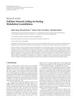
Báo cáo hóa học: " Research Article Process Neural Network Method: Case Study I: Discrimination of Sweet Red Peppers Prepared by Different Methods" pot

Hindawi Publishing Corporation
EURASIP Journal on Advances in Signal Pr ocessing
Volume 2011, Article ID 290950, 8 pages
doi:10.1155/2011/290950
Research Ar ticle
Process Neural Network Method: Case Study I:
Discrimination of Sweet Red Peppers Prepared by
Different Methods
Sevcan Unluturk,
1
Mehmet S. Unluturk,
2
Fikret Pazir,
3
and Alper Kuscu
4
1
Food Engineering Department, Izmir Institute of Technology, 35430 Izmir, Turkey
2
Department of Software Engineering, Izmir University of Economics, Sakarya Caddesi No. 156 Balcova, 35330 Izmir, Turkey
3
Food Engineering Department, Ege University, 35040 Izmir, Turkey
4
Faculty of Agriculture, Suleyman Demirel University, 32260 Isparta, Turkey
Correspondence should be addressed to Mehmet S. Unluturk,
Received 2 November 2010; Accepted 3 February 2011
Academic Editor: Enrico Capobianco
Copyright © 2011 Sevcan Unluturk et al. This is an open access article distributed under the Creative Commons Attribution
License, which permits unrestricted use, distribution, and reproduction in any medium, provided the original work is properly
cited.
This study utilized a feed-forward neural network model along with computer v ision techniques to discriminate sweet red pepper

products prepared by different methods such as freezing and pureeing. The differences among the fresh, frozen and pureed samples
are investigated by studying their bio-crystallogram images. The dissimilarity in visually analyzed bio-crystallogram images are
defined as the distribution of crystals on the circular glass underlay and the thin or the thick structure of crystal needles. However,
the visual description and definition of bio-crystallogram images has major disadvantages. A methodology called process neural
network (ProcNN) has been studied to overcome these shortcomings.
1. Introduction
Excluding analytical chemistry approaches for the evaluation
of food quality, there are numerous alternative methods
(holistic methods) that do not focus on the analysis of single
substances but regard foodstuffs as a whole. This approach
is based on the proposition that life itself is more than the
sum of its single constituent parts. The organization and
structure of food are important factors. The conservation of
this organization and structure is a sign of high food quality,
and structural decomposition is synonymous with plant
death. The purpose of complementary analysis methods is to
help characterize the vital activity [1]. The biocrystallization
method is one of the most important complementary
analysis methods.
Pfeiffer [2] originally introduced the term biocrystal-
lization, which is also called “sensitive crystallization” and
“copper chloride cr ystallization”. Engqvist [3] later initiated
the biocrystallization method. This method was developed
from the viewpoint that living organisms do not just exist as
substances, but have directing and organizing “structuring
forces” [ 4, 5]. These structuring forces direct the form and
function of the organism [6]. The method is based on
the crystallographic phenomenon that when adding specific
ionic substances, or in general all organic substances, to
an aqueous solution of dehydrate CuCl

2
, b iocrystallogr ams
with reproducible dendritic structures are formed during
crystallization. Crystallograms that are produced on the basis
of pure CuCl
2
exhibit a merely peripheral distribution of
crystals on the circular g lass underlay, with a diameter of
90 mm [4]. In contrast, biocrystallograms produced on the
basis of biological substances, such as plant extracts (fresh
sweet red pepper samples in this study), exhibit crystal
structures covering the entire glass underlay (Figure 1).
The biocrystallograms that are produced from agricul-
tural products, such as vegetables, grains, fruits, and milk
samples are based on three components: (a) an aqueous
solution or extract of the sample in question, (b) an aqueous
solution of dehydrate copper chloride, and (c) purified
water. Any kind of additive will change the copper chloride
2 EURASIP Journal on Advances in Signal Processing
(a) (b)
Figure 1: (a) Crystallogram obtained from basis of aqueous CuCl
2
·2H
2
O (blank). (b) Biocrystallogram obtained from conventionally grown
fresh sweet red pepper .
crystallization. The process is influenced by the qualitative
and quantitative variations in the macromolecules of the
biological extracts, thus allowing food quality assessment
[5]. When used to study human blood, t he results are

correlated with groups of pathologies and the concentration
of blood protein, and are predictive of worsening illnesses.
Early diagnosis seems possible in cancer research or in
occupational medicine (risk indicators) [7].
The phenomena of biocrystallograms are based on
ramification p atterns, which may be divided into three
major stages, extending from the center in all directions
to the periphery of the image (Figure 2). In the first or
1-zone biocrystallogram, when increasing concentrations of
agricultural extracts are applied relative to a given fixed
concentration of CuCl
2
, transparent needles with enormous
star-like formations extend in all directions to the periphery.
The second, 2-zone structure goes through the crystallization
center when it is divided by a vertical and horizontal axis. The
needles are pointed, predominantly transparent, and of rela-
tively equal length in the middle zone. These morphological
features may be described by means of plant morphological
terms, such as stems, branches, and needles. The last stage of
a biocrystallogram is an optimal degree divided into a 3-zone
structure with a center zone, middle z one, and marginal
zone. In t he third stage, a biocrystallogram exhibits various
macro and microscopic morphological features that reflect
the quality of the sample in question [5].
The biocrystallization method comprises two main parts
(Figure 3). The first is pattern formation, which starts in
a laboratory and continues until the crystallogram picture
is completely generated in the chamber. The s econd part
is pattern recognition. This is where the evaluation tools

will be responsible for perceiving and differentiating between
images [5].
There are two tools currently used to evaluate an image
visual evaluation and computerized image analysis. In visual
evaluation the images in question are evaluated based on the
judgment of a trained human using discrete reference scales
Figure 2: Biocrystallization method based on a phenomenon of
dendritic pattern formation during crystallization from an aqueous
solution containing plant extracts and CuCl
2
[2].
arranged in connection with picture phenomena. Comput-
erized image analysis interprets the image by using the
fundamental knowledge of texture analysis. Such techniques
have been explored and applied with the biocrystallization
method [5].
Computerized image analysis techniques may meet the
demand for such methods. Ideally, an image analysis proce-
dure should reflect all of the characteristics of a biocrystallo-
gram as a three-dimensional, colored ramification structure,
coordinated with zones relative to the center. However, due
to the present limitations set by computational capacity
and speed, simpler approaches are preferable. In a limited
number of previous studies, encouraging results have been
reported [4].
Computerized image analysis tools increase the objectiv-
ity of the method and allow the analysis of large numbers of
crystallization images [8]. This paper presents a unique neu-
ral network model, called process neural network (ProcNN),
EURASIP Journal on Advances in Sig nal Processing 3

Laboratory/chamber Evaluation tools
Pattern-formation Pattern-recognition
Figure 3: The detail of biocrystallization method [8].
along with computer vision techniques as an effective
analysis tool. The applicability of t his tool is tested for
discrimination of sweet red peppers (Capsicum annuum L.)
prepared by different methods such as freezing and pureeing.
As an effective computer vision technique, RGB (red, green,
blue) space is used since sweet red pepper fruit digital
images are c aptured and saved in RGB (red, green, blue)
space. For each component in RGB space, we performed
two calculations; the mean and standard deviation. The
mean characterizes the average color properties of sweet red
pepper, while standard deviation provides a measure of color
variation. Since three digital values assigned to every pixel of
sweet red pepper color image, 6 color features were extracted
for RGB color space, including the mean and the standard
deviation of each color component [9].
2. Sweet Red Pepper Extract and
Copper Chloride Concentrations
Conventionally grown sweet red pepper fruits (Capsicum
annuum L.) were obtained from Ege University Agricultural
Faculty Research, Applied and Production Farm in Menemen
(2005-2006; Izmir, Turkey). Fresh sweet red peppers were
quickly transferred to the laboratory. They were sorted,
cleaned, washed, dried, packaged under vacuum and frozen
at
−25
◦
C. They were stored at the same temperature until

used. The preparation steps of pureed samples include
removal of the stem and kernel parts of fresh peppers,
grating, thermal blanching at 95–100
◦
Cfor10minutes,hot
filling and sterilization at 115
◦
C for 20 minutes. Sterilized
pureed samples were refrigerated at 4
◦
Cuntilused.
In order to prepare sample extracts from fresh, frozen,
and sweet red peppers, the large peppers were initially
chopped into small pieces and passed through a kitchen type
blender (Braun MR 404, Hesse, Germany). The homogenate
was first passed through a cheese cloth to remove debris
particles and then filtered. The fruit juice was diluted to
1% with tridistilled water. CuCl
2
·2H
2
O solution was also
prepared at a 16% concentration with tridistilled water.
The optimal mixing ratio for the sample extract and cop-
per chloride influences the c rystallization pattern. Therefore,
the optimum sample and CuCl
2
·2H
2
O concentrations were

determined to be 1% and 16%, respectively.
For each biocrystallogram, a 1 mL sample (1% concen-
tration) was mixed with 3 mL CuCl
2
·2H
2
O (16% concen-
tration) per plate at chamber conditions of 25
◦
C and 55%
relative h umidity [11, 12]. The copper chloride was crystal-
lized after 16–18 hours. A total of 840 biocrystallograms were
produced from sweet red pepper fruit in 2005 and 2006. Only
single centered biocr ystallograms were evaluated, the others
(multicentered) were discarded.
2.1. Image Acquisition and Capture. Images were captured
using a digital camera model DMC-FZ5 (5 Mp) (Panasonic,
NJ, USA). The camera was positioned vertically over the
sample at a certain distance. The angle between the camera
lens, the lighting source, and ambient illumination were fixed
and kept the same for all the sample pictures. After that, the
images were transferred and stored in a PC as a JPEG format
of “high resolution” and “superfine quality”.
2.2. Image Processing. All the algorithms for preprocessing
of full images and image segmentation were written in
MATLAB 6.5 (The Math Works, Inc., MA, USA). MATLAB
code for pre-processing and i mage segmentation of a single
full image is given below:
s
= [


07.09.2006 taze Kristal 0

int2str(iStart)

.jpg

];
I
= imread(s);
D
= im2double(I);
r
= D(:,:,1);
g
= D(:,:,2);
b
= D(:,:,3);
r
= r(501:1100,351:1250);
g
= g(501:1100,351:1250);
b
= b(501:1100,351:1250);
d
= get coeffs2(r,g,b).
Inside get
coeffs2(r,g,b) function, the r, g, b values are
used to calculate the mean and the standard variation for red,
green,andblue components. Returned vector has six values

which correspond to RGB scale image. They are used as input
to the feed-forward neural network.
2.3. Image Segmentation. Each 1488
× 2240 pixel RGB
images was cropped to 600
× 900 pixel size (r = r(501:1100,
351:1250); g = g(501:1100,351:1250); b = b(501:1100,351:
1250));wherer, g, b is the red, green,andblue components).
These images were t hen used in t he decision process, as
the aim of these software-based procedures is to eventually
replace the human visual decision-making process.
3. Process Neural Network Architecture
Figure 4 shows a 1488 × 2240 RGB color biocrystallogram
images of fresh, pureed, and frozen sweet red peppers. In
these images, each pixel has three components corresponding
to Red, Green, and Blue. We reduced the image size to 600
× 900 (Figure 5), and then we calculated the mean and
standard deviation of Red, Green, and Blue components of
these images.
4 EURASIP Journal on Advances in Signal Processing
(a) (b)
(c)
Figure 4: Biocrystallogram images of (a) fresh, (b) pureed, and (c) frozen sweet red peppers [10].
As a result, we extracted 6 features for each image. These
features are the input to the feed-forward neural network.
There is one output node only whose value is
−0.9 if the
features belong to one type of class such as fresh sweet red
pepper fruit, or else 0.9 if the features belong to the other type
of class such as pureed sweet red pepper fruit. We chose 7 as

the number of hidden neurons. During the training phase,
if the learning does not get better, we will increment the
number of hidden neurons by two every other 400 epochs
[13]. For the training algorithm, we used back-propagation
algorithm [14–16]. Table 1 shows the training statistics for
the ProcNNs.
Epoch is defined as the presentation of the entire training
set to t he ProcNN, and sum-squared error is defined as a
measure of how well ProcNN is doing at a particular point
during its training [14–16]. For example, it took only 44
epochs to train the neural network for classification of fresh
and pureed samples. In the training phase, all the samples
(100%) were correctly classified by each neural network. Sum
squared error chosen for these neural networks was 0.009.
Figure 6 shows a fully interconnected feed-forward neural
network. It has six inputs, 7 hidden neurons and one output
neuron.
We examined the output statistics of the training phase
and decided to choose 0 as the decision factor (see Section 6).
The best performance that we obtained was from the
ProcNN for fresh and pureed samples. Testing output for
all 70 fresh samples was less than zero and for all 70
frozen samples, it was bigger than zero. We reached 100%
recognition.
There is also an alternative neural network approach for
the same problem. We can apply Bayes optimal decision rule
sincewehavetwoclassestoseparate[14]. Following section
discusses this method.
4. Bayes Opt imal Decision Rule
Classes are defined as:

H
0
= Fresh,
H
1
= Processed (pureed).
The prior probability of an unknown image being drawn
from class k is
h
k
(k
= 0,1). The cost of making a wrong
decision for class k is
υ
k
. Note that the prior probability
h
k
and the cost probability
υ
k
are taken as being equal,
EURASIP Journal on Advances in Sig nal Processing 5
(a) (b)
(c)
Figure 5: Reduced image size (600 × 900 pixel) for (a) fresh, (b) pur eed, and (c) fr ozen sweet red peppers.
Table 1: Training statistics for ProcNNs.
Neural network ty pe # of Epochs Sum-squared error Recognition
ProcNN (fresh and pureed) 44 0.009 100%
ProcNN (fresh and frozen) 70 0.009 100%

ProcNN (frozen and pureed) 29 0.009 100%
and hence can be ignored. The problem is to find a neural
network model for determining the class from which an
unknown image is taken. If we know the probability density
functions f
k
(
−→
X ) for all classes, the Bayes optimal decision
rule [14] can be used to classify
−→
X into class k if
h
k
ϑ
k
f
k

−→
X

>h
m
ϑ
m
f
m

−→

X

,(1)
where k
/
=m.
A major problem with (1) is that the probability
density functions of the classes are unknown. We can use
Gram-Charlier series expansion to estimate these unknown
probability density functions. In this case, the training set for
the neural network consists of Gram-Charlier coefficients.
Our objective in this study was to use these coefficients for
classification. If the neural network is trained with known
Gram-Charlier coefficients, then to determine the class of
an unknown image, we need only to feed its Gram-Charlier
coefficients. The next section describes the Gram-Charlier
series expansion.
5. Gram-Charlier Series
The Gram-Charlier series expansion of the probability d en-
sity function of a random variable with mean μ and variance
σ
2
can be represented as
ρ
(
x
)
=
1
σ

∞

i=0
c
i
φ
(i)

x − μ
σ

,(2)
where φ(x) is a Gaussian probability density function and
φ
(i)
(x)representstheith derivative of φ(x). For normalized
6 EURASIP Journal on Advances in Signal Processing
.
.
.
μ
R
σ
R
μ
G
σ
G
μ
B

σ
B
Bias
unit
Bias
unit
Frozen,ifoutput≥0
Fresh, if output <0
Figure 6: Process neural network (ProcNN) for fresh and pureed
samples.
1
1
1
23
4
j
L
Bias
unit
Bias
unit
Output
··· ···
W
0
11
W
0
1 j
W

0
1L
W
h
11
W
h
L1
W
h
L4
Λ
3
Λ
4
Λ
5
Λ
6
Gram-Charlier coefficients
Figure 7: Back propagation neural network. If output ≥0, then
input type of biocrystallogram sample image belongs to process
class (pureed) or it belongs to fresh class (where L is 19).
data where (μ = 0, σ
2
= 1, c
0
= 1), the above equation can
be simplified to
ρ

(
x
)
=

φ
(
x
)
+ c
3
φ
(3)
(
x
)
+ c
4
φ
(4)
(
x
)
+ c
5
φ
(5)
(
x
)

+c
6
φ
(6)
(
x
)
+
···

,
(3)
where c
i
coefficients are related to the central moments
of φ(x). In a sense, derivatives of the Gaussian function in
(3) provide us with the class type information for the sweet
red pepper. Furthermore, c
i
φ
(i)
are orthogonal functions that
present unique information about the process type sweet
red pepper class distribution. This leads us to conclude that
the procNN based on the decomposition of the probability
density function by the Gram-Charlier series is well suited for
fresh/processed (pureed) pepper class discrimination. Let’s
define β(x)as
β
(

x
)
=
1
√
2π
e
((−1/2)x
2
)
. (4)
−3 −2 −10123
0
0.1
0.2
0.3
0.4
0.5
0.6
0.7
0.8
0.9
1
Fresh class
Mashed class
(a)
−3 −2 −10123
0
0.1
0.2

0.3
0.4
0.5
0.6
0.7
0.8
0.9
1
Fresh class
Frozen class
(b)
−3 −2 −10123
0
0.1
0.2
0.3
0.4
0.5
0.6
0.7
0.8
0.9
1
Mashed class
Frozen class
(c)
Figure 8: Output density functions for training phase of (a) fresh-
pureed (shown as mashed) classes, (b) fresh-frozen classes, (c)
pureed (shown as mashed)-frozen classes.
EURASIP Journal on Advances in Sig nal Processing 7

Then, the probability density function becomes
ρ
(
x
)
= β
(
x
)

1+
1
6
Λ
3
A
3
+
1
24
(
Λ
4
− 3
)
A
4
+ ···

,(5)

where
A
i
(
x
)
= x
i
−
i
[2]
2 · 1!
x
i−2
+
i
[4]
2
2
· 2!
x
i−4
−
i
[6]
2
3
· 3!
x
i−6

+ ···,
i
[k]
=
⎛
⎝
i
k
⎞
⎠
=
i!
(
i
− k
)
!
,
m
k
=
1
n
n

i=1
[
x(i)
]
k

,
Λ
3
=−
m
3
− 3m
2
m
1
+2m
3
1
3!
,
Λ
4
=
m
4
− 4m
3
m
1
+6m
2
m
2
1
− 3m

4
1
4!
,
Λ
5
=−
m
5
− 5m
4
m
1
+10m
3
m
3
1
− 10m
2
m
3
1
+4m
5
1
5!
,
Λ
6

=
m
6
− 6m
5
m
1
+15m
4
m
2
1
6!
−
20m
3
m
3
1
+15m
2
m
4
1
− 5m
6
1
6!
.
(6)

Equation (6) is the so-called Gram-Charlier series [17]and
the polynomial A
i
(x) is called the Tchebycheff-Hermite
polynomial.
The training matrix was prepared using the Gram-
Charlier coefficients. Each column in the training matrix
represented one set of these Gram-Charlier coefficients with
a length of 4. Note that the amount of columns in the training
set could be any number. The bigger the number, the better
the discrimination achieved by the neural network for the
target biocrystallogram red pepper single centered images.
The results obtained when testing this neural network
show that biocrystallograms of sweet red pepper targets
can be detected with 56% accuracy. The number of hidden
neurons for the back propagation neural network was 19. It
took 2500 epochs for this neural network to train to reach
a sum-squared error of 0.009. In testing, if the output of
the output
≥ 0, then the input Gram-Charlier coefficients
belonged to class H
1
= processed (pureed). If the output
of the output <0, then the input Gram-Charlier coefficients
belonged to class H
0
= fresh (Figure 7).
Comparing ProcNN and Gram-Charlier neural network,
we can decide that representing images with Gram-Charlier
coefficients cause to lose the color information which is

important to detect the process types of the sweet red pepper.
On the other hand, ProcNN uses the mean and the color
variation of color components which helps the ProcNN reach
the performance between 85% and 100%.
6. Results
We created three ProcNNs. One ProcNN is used to classify
fresh and pureed, the second one is used to classify fresh and
frozen, and the last one is used to classify frozen and pureed
samples. The 1488
× 2240 pixel biocrystallogram images
were acquired in a lab and cropped to 600
× 900 pixel images
depicting either a fresh, pureed, or frozen sweet red pepper.
Within these images, a set of 140 images was utilized to train
each process neural network. Half of this set belonged to one
type of pepper class and the other half of the set belonged to
the other type of pepper class. A new set of 140 images was
then prepared to test each ProcNN performance in a similar
way.
Figure 8 shows the output training statistics for fresh
and pureed, fresh and frozen, and pureed and frozen
sweet pepper samples. We chose 0 as the decision factor
(Figure 8(a)). During testing this Pr ocNN for discrimination
of fresh and pureed samples, any output whose value is
greater and equal to 0, we decide the sample belongs to
pureed class; otherwise it belongs to fresh class. Testing
output for all 70 fresh samples was less than zero, and for all
70 frozen samples, testing o utput was bigger than zero. We
reached 100% recognition.
We also chose 0 as the decision factor for ProcNN in

the fresh and frozen samples (Figure 8(b)). During testing
this ProcNN, any output whose value is greater and equal
to 0, we decide the sample belongs to frozen class; otherwise
it belongs to Fresh class. Testing output for 63 out of 70
fresh samples was less than zero, and for 65 out of 7 0 frozen
samples, testing output was bigger than zero. We reached
92% recognition.
For discrimination of fresh and frozen samples, we also
chose 0 as the decision factor for this procNN (Figure 8(c)).
During testing this ProcNN, any output whose value is
greater and equal to 0, we decide the sample belongs to fresh
class; otherwise it belongs to frozen class. Testing output for
57 out of 70 fresh samples was less than zero, and for 62 out
of 70 frozen samples, testing output was bigger than zero. We
reached 85% recognition.
This high level of recognition suggests that ProcNN
methodology and color measurements obtained from RGB
color space is a promising method for the discrimination
of sweet red pepper products prepared by different methods
using its biocrystallogram images.
7. Conclusion
In this study, we developed a neural network to determine
whether sweet red peppers are processed or not. We use
biocrystallogram images of sweet red peppers for this
neural network model since these images taken from a lab
bear information related to the process type of pepper.
However, this information is not readily quantifiable and
lacks uniquely recognizable features. Therefore, a neural
network becomes appealing for classifying these images,
because neural network is trainable. The optimal values for

the neural network weights were estimated using the back
propagation algorithm. Experimental measurements of the
8 EURASIP Journal on Advances in Signal Processing
pepper were utilized to t rain and test the process neural
network. This network showed a remarkable 100% clas-
sification performance. P arallel classification performance
was also achieved when training the neural network. These
results are encouraging and su ggest that neural ne tworks
are potentially useful for discriminating sweet red peppers
processed by different methods. Furthermore, the process
neural network renders practical advantages such as real-
time processing, adaptability, and training capability. It is
important to point out that similar neural network designs
can be used in classification of food grains’ images, detection
of contaminated food products, evaluating the surface qual-
ity of food raw materials, determination of quality features
of foods, such as object recognition, geometrical parameters,
surface colour, and in other areas such as medical ultrasonic
imaging for tissue characterization and diagnosis, industrial
defect discrimination, and so forth.
References
[1] W. Harms, “Quality of organic food,” Genetic Engineering
Newsletter -Special Issue, vol. 16, pp. 1–11, 2004.
[2] E. Pfeiffer, Studium von Formkr¨aften an K ristallizationen,
Naturwissenschaftliche Sektion am Goetheanum, Dornach,
Switzerland, 1931.
[3] M. Engqvist, Gestaltkrafte des Lebendigen, Klostermann,
Frankfurt am Main, Germany, 1970.
[4] J. O. Andersen, C. B. Henriksen, J. Laursen, and A. A. Nielsen,
“Computerised image analysis of biocrystallograms originat-

ing from agricultural products,” Computers and Electronics in
Agriculture, vol. 22, no. 1, pp. 51–69, 1999.
[5] A. Meelursarn, Statistical evaluation of texture analysis from
the biocrystallization method: effect of image parameters to
differentiate samples from different farming systems,Doctoral
dissertation, University of Kassel, Department of Organic
Food Quality and Food Cultur e, Witzenhausen, Germany,
December 2006.
[6] J.Bloksma,M.Northolt,andM.Huber,Parameters for Apple
Quality Part-1, Louis Bolk Institute, 2001.
[7] J. G. Barth, “Cristallisation avec additif, cas particulier du
chlorure cuivrique et de ses applications,” Phytoth´erapie,vol.
2, no. 6, pp. 183–190, 2004.
[8] P. Doesburg and M. Huber, “Biocrystallisation and Steigbild
results at the Louis Bolk Instituut,” Elemente Der Naturwis-
senschaft, no. 87, pp. 118–123, 2007.
[9] C. Zheng, D W. Sun, and L. Zheng, “Correlating colour to
moisture content of large cooked beef jo ints by computer
vision,” Journal of Food Engineering, vol. 77, no. 4, pp. 858–
863, 2006.
[10] A. Kuscu, Organik ve Konvansiyonel Kırmızıbiber ve
¨
Ur¨unlerinin Ayırt Edilebilme Y¨ontemleri ve Kalite
¨
Ozelliklerinin
˙
Incelenmesi,Ph.D.thesis,Ege
¨
Universitesi Fen Bilimleri
Enstit

¨
us
¨
u, Izmir, Turkey, 2008.
[11] U. R. Balzer-Graf, U. K
¨
opke, and U. Geier, “Research on
Quality in Organic Agriculture by P icture Forming Methods,
Understanding the Quality of Organic Horticultural Products
(Short Course on),” Izmir, Turkey, May 2001.
[12] M. Szulc, F. Cordeiro, A. Maquet, and E. Anklam, “Application
of a multivariate design approach for maximisation of the
observed differences between organically and conventionally
grown wheat grains in biocrystallisation method,” in Pro-
ceedings of the 1st Scientific FQH Conference, p. 78, Fibl,
Switzerland, November 2005.
[13]M.Islam,A.Sattar,F.Amin,X.Yao,andK.Murase,“A
new adaptive merging and growing algorithm for designing
artificial neural networks,” IEEE Transactions on Systems, Man,
and Cybernetics B, vol. 39, no. 3, pp. 705–722, 2009.
[14] T. Masters, PracticalNeuralNetworks,AcademicPress,New
York, NY, USA, 1993.
[15] A. Cichocki and R. Unbehauen, Neural Networks for Optimiza-
tion and Signal Processing, John Wiley & Sons, New York, NY,
USA, 1992.
[16] J. A. Freeman and D. M. Skapura, Neural Networks Algorithms,
Applications, and Programming Techniques, Addison-Wesley,
1991.
[17] M. W. Kim and M. A rozullah, “Generalized probabilistic
neural network based classifiers,” in Proceedings of the Interna-

tional Joint Conference on Neural Networks, vol. 3, pp. 648–653,
1992.