Báo cáo hóa học: "Research Article Digital Communication Receivers Using Gaussian Processes for Machine Learning" ppt

Hindawi Publishing Corporation
EURASIP Journal on Advances in Signal Processing
Volume 2008, Article ID 491503, 12 pages
doi:10.1155/2008/491503
Research Article
Digital Communication Receivers Using Gaussian Processes for
Machine Learning
Fernando P
´
erez-Cruz
1, 2
and Juan Jos
´
e Murillo-Fuentes
3
1
Department of Electrical Engineering, Princeton University, Princeton, NJ 08544, USA
2
Department of Signal Theory and Communications, Carlos III University of Madrid, Avda. Universidad 30, 28911 Legan
´
es, Spain
3
Depar t amento de Teor
´
ıa de la Se
˜
nal y Comunicaciones, Escuela T
´
ecnica Superior de Ingenieros, Universidad de Sevilla,
Paseo de los Descubrimientos s/n, 41092 Sevilla, Spain
Correspondence should be addressed to Fernando P

´
erez-Cruz,
Received 13 October 2007; Revised 18 March 2008; Accepted 19 May 2008
Recommended by An
´
ıbal Figueiras-Vidal
We propose Gaussian processes (GPs) as a novel nonlinear receiver for digital communication systems. The GPs framework can
be used to solve both classification (GPC) and regression (GPR) problems. The minimum mean squared error solution is the
expectation of the transmitted symbol given the information at the receiver, which is a nonlinear function of the received symbols
for discrete inputs. GPR can be presented as a nonlinear MMSE estimator and thus capable of achieving optimal performance from
MMSE viewpoint. Also, the design of digital communication receivers can be viewed as a detection problem, for which GPC is
specially suited as it assigns posterior probabilities to each transmitted symbol. We explore the suitability of GPs as nonlinear digital
communication receivers. GPs are Bayesian machine learning tools that formulates a likelihood function for its hyperparameters,
which can then be set optimally. GPs outperform state-of-the-art nonlinear machine learning approaches that prespecify their
hyperparameters or rely on cross validation. We illustrate the advantages of GPs as digital communication receivers for linear and
nonlinear channel models for short training sequences and compare them to state-of-the-art nonlinear machine learning tools,
such as support vector machines.
Copyright © 2008 F. P
´
erez-Cruz and J. J. Murillo-Fuentes. This is an open access article distributed under the Creative Commons
Attribution License, which permits unrestricted use, distribution, and reproduction in any medium, provided the original work is
properly cited.
1. INTRODUCTION
Gaussian processes are typically used to characterize the
noise component in digital communication systems, as it
is mainly caused by thermal noise fluctuations [1]. In this
paper, we propose the Gaussian processes (GPs) framework
to design nonlinear receivers in digital communication sys-
tems. GPs were initially presented as a nonlinear estimation
technique in 1978 [2] and were rapidly forgotten due to

its computation complexity. In the mid-nineties, they were
independently rediscovered [3]. Since then, they have been
shown to fit many different applications [4] and nowadays
their computational complexity is no longer a limiting issue
[5].
There is a vast literature on machine learning techniques
for designing digital communication systems. The channel
equalization problem has been addressed with different
machine learning tools, such as multilayered perceptrons
(MLPs) [6], radial basis function networks (RBFNs) [7],
recurrent RBFNs [8], self-organizing feature maps (SOFMs)
[9],waveletneuralnetworks[10], GCMAC [11], kernel
adaline (KA) [12], or support vector machines (SVMs)
[13], among many others. Other digital communication
systems that have also benefited from nonlinear detection
and estimation algorithms are multiuser detection [14, 15],
multiple-input multiple-output systems [16], beam forming
[17], predistortion [18], and plant identification [19], to
name a few.
For these machine learning approaches, it is necessary to
prespecify the hyperparameters (structure), since standard
methods for searching the optimal hyperparameters (i.e.,
cross-validation [20, 21]) require immense computational
resources, which are not available in most communication
receivers, and also their training time is highly variable.
As a result, they use a suboptimal structure that requires
longer training sequences for ensuring optimal receiver
2 EURASIP Journal on Advances in Signal Processing
performance. Also, it makes the length of the training
sequence hard to predict, as it depends on how well the

chosen structure or hypeparameters fits the current problem.
For example, SVM with a Gaussian kernel needs to fit its
width, which is proportional to the noise level [12, 13, 22]. If
the width is too large, the SVM can be optimized with short-
training sequences, but its performance is poor. If it is too
small, it requires a significantly longer training sequence to
avoid overfitting. For each instantiation of the problem, there
is an optimal width. This kernel width depends not only on
the channel values and noise level, as we would expect, but
also on the actual values of the noise themselves. Ideally, we
would like to choose the kernel width every time we receive
a new training sequence. But this would involve training a
different SVM for each possible width and then choosing the
optimal receiver (validation). In addition, this width is not
the only SVM’s hyperparameter. We must also validate the
soft margin that trades off the minimization of the training
errors and the maximization of the margin. Therefore, we
wouldhavetotrainasetofreceiverswithdifferent width and
soft-margin hyperparameters to find the optimal setting in
each problem. However, typically, we can only solve a single
optimization problem in the receiver. We thus prespecify the
SVM hyperparameters, as it is the case with other nonlinear
tools referenced earlier.
In previous work, we introduced Gaussian processes for
machine learning as a novel nonlinear tool for designing
digital communication receivers. Gaussian processes can
be applied to regression and classification problems [4],
and in this paper we use both settings for tuning digital
communication receivers with short training sequences.
We compare Gaussian processes for regression (GPR) and

Gaussian processes for classification (GPC) to state-of-the-
art linear and nonlinear receivers to show their strength
in solving this relevant problem. We have presented some
preliminaries results for multiuser detection in CDMA
systems [23, 24] and channel equalization in [25]. In this
paper, we extend these results and include GPC in our
comparisons.
Gaussian processes for machine learning are rooted in
Bayesian statistics [4], and consequently build a likelihood
function for its hyperparameters given the training examples.
This likelihood can be optimized to set the hyperparameters.
This property makes GPs an attractive tool for designing
nonlinear digital communication receivers, compared to
other nonlinear machine learning tools, because the hyper-
parameters can be optimally set for each instantiation of our
problem with a single optimization procedure.
For short training sequences, hyperparameter mismatch
significantly affects the performance of digital communi-
cation receivers, while for longer training sequences, this
performance is not sensitive to variations in the hyperpa-
rameters. Most papers applying nonlinear machine learning
for designing digital communication receivers propose fixed
hyperparameters and sufficiently long training sequences.
We focus on short-training sequences and show that fixed
hyperparameters underperform compared to GPR receivers
with optimally trained hyperparameters.
Gaussian processes can be extended for solving classi-
fication problems. In this case, the posterior is no longer
tractable and we need to use approximations to compute the
prediction for each class label [4]. A Gaussian distribution

is typically used to approximate the GPC’s posterior, either
using Laplace [26] or expectation propagation methods [27].
However, GPC computational complexity is significantly
higher than that of GPR, and hence they might not be as
suited for designing digital communication receivers as GPR.
Moreover, their performance is not as good as that of GPR
receivers as we show and explain in the experimental section.
The rest of the paper is organized as follows. We
present the design of digital communication receivers as an
optimization problem in Section 2 and show how different
nonlinear machine learning tools can be fitted in this
framework. Section 3 is devoted to Gaussian processes for
regression and how it can be understood as a nonlinear
MMSE estimation. The optimization of the GPR hyperpa-
rameters is proposed in Section 4. Section 5 introduces GPC
briefly. We present some computer simulations in Section 6
to illustrate the benefits of GPR for channel equalization
and multiuser detection compared to other state-of-the-art
nonlinear tools. We conclude with some final remarks and
proposed further work in Section 7.
2. NONLINEAR OPTIMIZATION FOR
COMMUNICATION RECEIVERS
2.1. Channel model and MMSE
We consider throughout the paper the following determinis-
tic channel model:
x
= Hs + z,(1)
where s is a random variable column-vector representing
the transmitted symbols, H corresponds to the deterministic
channel gains, unknown to both the transmitter and receiver,

z is zero-mean Gaussian noise, and x represents the received
symbols. This model is general enough to capture most
standard communication systems.
(i) Intersymbol interfe rence: each element in s is a symbol
transmitted at a different time instant. H is a Toeplitz matrix,
in which each row represents the channel impulsive response.
(ii) Multiple-input multiple-output: (H)
ij
represents the
gain from the ith receiving antenna to the jth transmitting
antenna and s represents the symbols transmitted by the
antenna array.
(iii) Fading: H is a diagonal matrix with the fading coef-
ficients and s represents the symbols transmitted at each time
instant.
(iv) CDMA: the columns of H collect each user’s spread-
ing code and each element of s represents the symbol
transmitted by the users.
We can also combine different H matrices to accom-
modate other communication systems. For example, H
=
H
1
H
2
H
3
,whereH
1
is a Toeplitz matrix representing an

intersymbol interference channel model, H
2
contains the
spreading codes of a CDMA system, and H
3
is a diagonal
matrix assigning different power to each user. This H matrix
F. P
´
erez-Cruz and J. J. Murillo-Fuentes 3
represents the downlink channel in a mobile communication
network.
The source s that achieves capacity (maximum infor-
mation transmission rate) [28] is a zero-mean Gaussian
distribution with a covariance matrix given by the right
eigenvectors of the channel matrix [29]. s being a continuous
random variable, we can estimate in the receiver the
transmitted vector using a minimum mean squared error
(MMSE) detector:
f
mmse
(x) = arg min
f (·)
E



s − f (x)



2

. (2)
The function f
mmse
(x) is the mean value of s given the
received vector x, E[s
| x], which is a linear function of x
if s is Gaussianly distributed. Practical structural constraints
dictate the use of discrete constellations, such as PSK and
QAM, which depart from the optimal Gaussian distribu-
tions. Although linear detectors cannot achieve E[s
| x]if
s is a discrete random variable, and thus the MMSE is only a
proxy for minimizing the probability of misclassification, still
digital communication receivers use linear MMSE detectors
for estimating the transmitted vector, because they can
be easily implemented and hopefully their performance is
not severely degraded. For example, if s
∈{±1} and
equiprobable and H
= 1, then E[s | x] = tanh(x/σ
2
z
). The
linear MMSE solution is given by
w
mmse
= arg min
w

E


s − w

x

2

=

E

xx


−1
E[xs].
(3)
If H is unknown, we can replace the expectations by sample
averages using a training sequence.
2.2. Machine learning for digital
communication receivers
The design of digital communication receivers can be readily
understood as a supervised classification problem [6, 30], in
which the receiver constructs a classifier for deciding over the
incoming symbols. Machine learning tools optimize the risk
of misclassification:
f
opt

(x) = arg min
f (·)
E

L

s, f (x)

=
arg min
f (·)

L

s, f (x)

p(s, x)ds dx,
(4)
where L(
·) is a loss function that measures the penalty for
wrongly classifying a pattern, and f (x) is the nonlinear
model to predict s.
The joint density, p(s, x), is typically unknown, and thus
we use a training sequence
{x
i
, s
i
}
n

i
=1
and the empirical risk
minimization (ERM) inductive principle [31] to obtain the
optimal solution:

f
opt
(x) = arg min
f (·)

n

i=1
L

s
i
, f

x
i

+ λΩ


f 


,(5)

where we have included a regularization term, λΩ(
f ),
to avoid overfitting and to ensure that the minimum of
the empirical risk converges to the minimum risk [31]as
the number of training samples increases. The number of
training patterns n determines the symbols in the preamble
of each transmission needed to adjust the receiver. This
number should be small to maximize the number of bits
used to transmit information, as we need to retransmit the
preamble in each burst of data.
The nonlinear machine learning approaches mentioned
in the introduction can be cast as the optimization in (5)
using an appropriate nonlinear model, loss function, and
regularizer. For example, f (x)
= w

φ(x), where φ(x)is
a nonlinear transformation to a higher-dimensional space;
L(s
i
, f (x
i
)) = (1 − s
i
w

x
i
)
+

, hinge loss, where (y)
+
=
max(y,0); and Ω(f ) =w
2
weight decay [21]givesan
SVM for a binary antipodal constellation, which constructs
the nonlinear classifier using the “kernel trick” for φ(
·)[32].
The convexity of the optimization in (5) depends on
f (
·), L(·, ·), and Ω(·). In some cases, as in SVM or KA, it
leads to a convex functional and in others, as in MLP or
RBFN, it does not. But in any case, these machine learning
approaches rely on an iterative optimization tool [21, 32]for
solving (5).
If we choose f (x)
= w

φ(x), L(s, f (x)) = (s − w

φ(x))
2
and Ω( f ) =w
2
,wegetaconvexfunctional:
w
nl mmse
= arg min
w


n

i=1

s
i
−w

φ

x
i

2
+ λw
2

(6)
that can be analytically optimized as
w
nl mmse
=

Φ

Φ + λI

−1
Φ


s,(7)
where Φ
= [φ(x
1
), , φ(x
n
)]

and s = [s
1
, , s
n
]

.
We denote this solution as nonlinear MMSE, since it is a
nonlinear extension of (3), in which we have substituted x
by φ(x) and we have replaced the expectations by sample
averages.
In the next section, we show (7) is equivalent to the
mean solution provided by Gaussian processes for regression
with a Gaussian likelihood function and that it can be solved
using kernels [33]. Moreover, interpreting (7) as GPR allows
optimizing its hyperparameters by maximum likelihood
(Section 4). This optimization improves the performance
of (7) with respect to other nonlinear machine learning
procedures when the number of training samples is low,
because for reduced training datasets the performance of
nonlinear machine learning methods significantly depends

on its hyperparameters.
3. GAUSSIAN PROCESSES FOR REGRESSION
In the past few years, a new Bayesian machine learning tool
based on Gaussian processes (GPs) has been developed for
nonlinear regression estimation [3, 4, 34]. In a nutshell,
Gaussian processes for regression (GPR) assume that a GP
prior governs the set of possible regressors. Consequently,
the joint distribution of training and test data is given
by a multidimensional Gaussian density function, and the
predicted distribution for each test point is estimated by
conditioning on the training data.
4 EURASIP Journal on Advances in Signal Processing
We present GPR from the Bayesian generalized linear
regression viewpoint. Although from this opening we lose
the GPs interpretation and we can only work with Gaus-
sian likelihood models, we believe it is a simpler way to
understand GPR. This approach mimics how most machine
learning textbooks introduce nonlinear regression [21, 32,
35] and it helps understanding GPR as a nonlinear MMSE
estimation. Therefore, practitioners in signal processing for
digital communications can readily relate to this new tool for
estimation and detection. Both interpretations are described
in [34], where they are shown to be identical for Gaussian
likelihood models. There is more about GPs than what
we introduce in this summary, for interested readers, GPs
extensions can be found in [4].
A generalized linear regressor expresses the input-output
relation as
s
= w


φ(x)+ν,(8)
where φ(
·) is a nonlinear transformation to a higher-
dimensional feature space and ν is a random variable that
measures the deviation between s and its estimate. Given a
labeled training sequence (D
={x
i
, s
i
}
n
i
=1
, where the input
x
i
∈ R
d
and the output s
i
∈ R) and a statistical model for
ν, we can compute the regressor w by maximum likelihood
(ML),
w
ML
= arg max
w
n


i=1
p

ν
i

=
arg max
w
n

i=1
p

s
i
−w

φ

x
i

.
(9)
We use these ML weights to predict the outputs for future
test points x
∗
:

s
∗
= w

ML
φ

x
∗

. (10)
In Bayesian machine learning, w is considered to be a
random variable and, to predict the outcome of x
∗
,weuse
its conditional density given the training dataset, p(w
| D).
This conditional density, known as the posterior of w,canbe
computed through Bayes rule,
p(w
| D ) = p(w | s, X) =
p(s | X, w)p(w)
p(s | X)
=
p(w)
p(s | X)
n

i=1
p


s
i
| x
i
, w

,
(11)
where p(s
i
| x
i
, w) is the likelihood function of w, p(w)its
prior distribution and X
= [x
1
, , x
n
]

.
To predict the output for a new test point x
∗
we integrate
out w:
p

s
∗

| x
∗
, D

=

W
p

s
∗
| x
∗
, w

p(w | D )dw, (12)
in which the conditional density of each s
∗
(the likelihood of
w) is weighted by the posterior of w and is summed over all
possible w. As a result, we get a full statistical description of
s
∗
, given all the available information (x
∗
and D). In this
setting, we predict the value of s
∗
using the full statistical
model of w, not only its maximum likelihood estimate.

This setting is quite general, as we can use any model for
the likelihood and prior for solving the regression estimation
problem. Gaussian likelihood, p(s
| x, w) = N (w

φ(x),σ
2
ν
),
leads to the MMSE criterion, and a zero-mean Gaussian
prior, p(w)
= N (0, σ
2
w
I), allocates probability mass to every
possible w and allows solving (12)analytically.Theposterior
distribution in (11) is then a Gaussian density function,
p(w
| D ) = N (μ
w
, Σ
w
), where
μ
w
= σ
2
w

σ

2
w
Φ

Φ + σ
2
ν
I

−1
Φ

s, (13)
Σ
−1
w
=
Φ

Φ
σ
2
ν
+
I
σ
2
w
. (14)
Actually, the posterior mean in (13) is identical to the

maximum a posteriori (MAP) of (11):
μ
w
= w
MAP
= arg max
w

p(w | s, X)

=
arg max
w

log p(s | X, w) + log p(w)

=
arg max
w

−
1
σ
2
ν
n

i=1

s

i
−w

φ

x
i

2
−
1
σ
2
w
w
2

,
(15)
which is identical to (6)forλ
= σ
2
ν
/σ
2
w
. We can also check
that (13)isequalto(7). Therefore, the GPR mean prediction
can be regarded as a nonlinear MMSE estimation for the
nonlinear mapping φ(

·).
The prediction for s
∗
in (12) is a Gaussian density
function, p(s
∗
| x
∗
, D) = N (μ
s
∗
, σ
s
∗
):
μ
s
∗
= φ


x
∗

μ
w
= φ


x

∗

Σ
w
Φ

s
σ
2
ν
, (16)
σ
2
s
∗
= φ


x
∗

Σ
w
φ

x
∗

=
φ



x
∗


Φ

Φ
σ
2
ν
+
I
σ
2
w

−1
φ

x
∗

.
(17)
There is an alternative formulation for μ
s
∗
and σ

2
s
∗
,in
which we do not need to know the nonlinear mapping φ(
·)
and we only need to work with its inner product or kernel,
defined as
k

x
i
, x
j

=
σ
2
w
φ


x
i

φ

x
j


. (18)
To obtain this alternative formulation, we first define the
covariance matrix C as
(C)
ij
= k

x
i
, x
j

+ σ
2
ν
δ
ij
, (19)
which can be related to Σ
w
as follows:
Σ
−1
w
Φ

=

Φ


Φ
σ
2
ν
+
I
σ
2
w

Φ

=
Φ


σ
2
w
ΦΦ

+ σ
2
ν
I


σ
2
ν

σ
2
w

=
Φ

C

σ
2
ν
σ
2
w

.
(20)
F. P
´
erez-Cruz and J. J. Murillo-Fuentes 5
Now if we premultiply (20)byΣ
w
and postmultiply it
by C
−1
, we obtain the following equivalency: Σ
w
Φ


/σ
2
ν
=
σ
2
w
Φ

C
−1
, which can be used to simplify (16)andexpress
the GPR prediction mean as
μ
s
∗
= φ


x
∗

σ
2
w
Φ

C
−1
s = k


C
−1
s, (21)
where
k
= σ
2
w
φ


x
∗

Φ

=

k

x
∗
, x
1

, , k

x
∗

, x
n


. (22)
To compute the prediction for any vector x
∗
,wedonot
need to know the nonlinear mapping φ(
·), only its kernel.
The complexity of computing μ
s
∗
in (21) is linear, because we
can precompute the vector C
−1
s that does not depend on x
∗
and we only need to filter k with it for each new test pattern.
We can also define the variance of our predictor using
kernels as
σ
2
s
∗
= k

x
∗
, x

∗

−
k

C
−1
k, (23)
which is achieved after applying to (14) the matrix inversion
lemma described in [36].
Equations (21)and(23) represent the predictions for x
∗
given by the Gaussian processes view of GPR. The matrix
C is the covariance matrix of a multidimensional Gaussian
distribution, hence its name, that describes the training data,
and the vector k represents the covariance vector between the
training dataset and the test vector. Therefore, the function
k(
·, ·) has to be a positive-definite function to ensure that
the Gaussian processes covariance matrix C is also positive
definite.
4. HYPERPARAMETER OPTIMIZATION
If either φ(
·)ork(·, ·) is known, we can analytically predict
the output of any incoming sample using (21). But for most
estimation problems, the best nonlinear transformation (or
its kernel) is unknown. As discussed in the Section 2, the
optimal setting of the hyperparameters could be obtained by
cross-validation, similarly to any other nonlinear machine
learning method. In this case, the nonlinear MMSE would

be as good as any of the other methods, as it would require
eithertotrydifferent settings or to rely on a prespecify one.
From the point of view of Bayesian machine learning,
we can proceed as we did for the parameters w in Section 3.
First, we compute the likelihood of the hyperparameters of
the kernel given the training dataset:
p(s
| X, θ) =

p(s | wX, θ)p(w | D ,θ)dw
=
1

(2π)
n


C
θ


exp

−
1
2
s

C
−1

θ
s

,
(24)
where θ represents the hyperparameters of the covariance
function or kernel. We have added θ to the covariance matrix,
likelihood, and posterior to explicitly indicate that they
depend on the kernel’s hyperparameters. This was omitted
in the GPR presentation in Section 3 for clarity purposes.
Second, we can define a prior for the hyperparameters,
p(θ), that can be used to construct its posterior density:
p(θ
| D ) =
p(s | X, θ)p(θ)
p(s | X)
. (25)
Third, we can integrate out the hyperparameters to
obtain the predictions:
p

s
∗
| x
∗
, D

=

p


s
∗
| x
∗
, Dθ

p

θ | D

dθ. (26)
However, in this case, the hyperparameters’ likelihood
does not have a conjugate prior and the posterior is
nonanalytical. Hence the integration has to be done either
by sampling or approximations. Although this approach
is well principled, it is computational intensive and it
is not feasible for digital communications receivers. For
example, Markov-chain Monte Carlo (MCMC) methods
require several hundreds to several thousands samples from
the posterior of θ to integrate it out in (26). For the interested
readers, further details can be found in [4].
Alternatively, we can use the likelihood function of the
hyperparameters and compute its maximum to obtain its
optimal setting [3], which is used to describe the kernel for
the test samples. Although setting the hyperparameters by
maximum likelihood is not a purely Bayesian solution, it is
fairly standard in the community and it allows using Bayesian
solutions in time-sensitive applications. The maximum
likelihood hyperparameters are given by

θ
ML
= arg max
θ
p(s | X, θ)
= arg max
θ
log p(s | X, θ)
= arg max
θ

−
s

C
−1
θ
s − log


C
θ



.
(27)
This optimization is nonconvex [37]. But as we increase
the number of training samples, the likelihood becomes
a unimodal distribution around the maximum likelihood

hyperparameters and the ML solution can be found using
gradient ascent techniques. See [4] for further details.
4.1. Covariance matrix
To optimize the kernel hyperparameters in (27), we need
to describe a kernel in a parametric form. Kernel design
is one of the most challenging open problems in machine
learning, as it is mainly driven by each particular application.
We need to incorporate our prior knowledge into the kernel,
but, at the same time, we want the kernel to be flexible to
explain previously unknown trends in the data. In [4], a list
of flexible kernels, (i.e., linear, Gaussian, neural networks,
Mat
´
ern, among others; and their properties are described).
The rules on how to combine them are also described,
(i.e., the sum or product of two kernel functions is also a valid
kernel function).
For example, if we know the optimal solution to be linear,
we could use the linear kernel: k(x, x
) = σ
2
w
x

x.Theonly
unknown hyperparameters in this case are σ
2
ν
and σ
2

w
,as
6 EURASIP Journal on Advances in Signal Processing
we do not need to know these variances a priori. In the
remaining of this text, we consider, without loss of generality,
the last term in (19) to be part of the designed kernel, as δ
ij
is a valid kernel and the weighted sum of kernel functions
(with nonnegative weights) is also a kernel. In general,
kernel functions are more complex and they incorporate
several hyperparameters. For example, the Gaussian kernel
with automatic relevance determination (ARD) proposes
one nonnegative weight, γ

, per input dimension:
k

x
i
, x
j

=
α
1
exp

−
d


=1
γ


x
i
−x
j

2

+ α
2
x

i
x
j
+ α
0
δ
ij
,
(28)
where we have added a linear kernel to use this covariance
function for designing digital communication receivers. For
this kernel function we define the hyperparameters as θ
=
[log α
0

,logα
1
,logα
2
,logγ

], because these hyperparameters
need to be positive to ensure that k(
·, ·)isapositive
semidefinite function. Hence, we can apply unconstrained
optimization tools if we work over θ.
The covariance function in (28) is a good kernel
for designing digital communication receivers using GPR,
because it contains a linear and a universal nonlinear part,
as the RBF kernel has an infinite VC dimension [31]. The
linear part can mimic the best linear decision boundary and
the nonlinear part modifies it, where the linear explanation
is not optimal to obtain the expectation of s given x.If
the channel is linear, then the ML solution sets α
1
= 0
and there is no interference of the nonlinear term with the
nonlinear one in the solution. Also, using a radial basis
kernel for the nonlinear part seems an appropriate choice
to achieve nonlinear decisions for digital communication
receivers, because the received symbols form a constellation
of clouds of points with Gaussian spread around its centers.
4.2. Discussion
Gaussian Processes for regression is a nonlinear regres-
sion tool that, given the covariance function, provides an

analytical solution to any regression estimation problem.
Moreover, it does not only give point estimates, but it also
assigns confidence intervals for them. In GPR, we perform
the optimization step to set the covariance function hyper-
parameters by maximum likelihood, unlike SVM or other
nonlinear machine learning tools, in which the optimization
is used to set the optimal parameters. In these methods, the
hyperparameters have to be either prespecified or estimated
by cross-validation [20].
Cross-validation optimizes several functionals (typically
less than 10) for each possible setting of the hyperparameters
[21]. The number of hyperparameters that can be tuned
is quite limited (at most 2 or 3), as the computational
complexity of cross-validation increases exponentially with
the number of hyperparameters. These remarkable draw-
backs limit the application of these nonlinear tools to digital
communications receivers, since we face complex nonlinear
problems with reduced computational resources and short-
training sequences. By exploiting the GPs framework, as
stated in this paper, we can avoid them.
5. GAUSSIAN PROCESS FOR CLASSIFICATION
Gaussian process for classification is a bit trickier than the
regression counterpart, because we cannot rely on a Gaussian
likelihood function to predict the labels of each class as the
outcomes come from a discrete set [4]. Thereby to predict
the class labels, we need to resort to numerical integration
or approximations to tractable density models. A generalized
linear binary classifier predicts for an input x the class label
as follow:
p(s

= +1 | w, x) = p(s = +1 | f ) = σ( f ), (29)
where f
= w

φ(x) is an underlying continuous function,
σ(
·) is a sigmoid that squashes f between 0 and 1, and p(s =
−
1 | f ) = 1 − p(s = +1 | f ). σ(·) is typically the logistic
function or the cumulative density function of a Gaussian
[4].
Given a labeled training sequence (D
={x
i
, s
i
}
n
i
=1
,where
the input x
i
∈ R
d
and the output s
i
∈{±1}), we can
compute the posterior over the underlying function f
=

[ f
1
, , f
n
]

using Bayes rule, as we did in Section 3 for GPR
with w, and we can integrate out f to predict the class label
for any new test point x
∗
. We can compute the class label for
the test samples as follows:
p

s
∗
= +1 | x
∗
, D

=

σ

f
∗

p

f

∗
| x
∗
, D

df
∗
, (30)
where
p( f
∗
| x
∗
, D) =

p( f
∗
| x
∗
, X, f)p(f | D )df, (31)
p(f
| D ) = p(f | X, s) =

i
p

s
i
| f
i


p(f | X)
p(s | X)
. (32)
In (31), we compute the distribution for the underlying
function in the test point and in (30) we integrate out the
underlying function to predict the probability that the class
label of that point is +1. Both integrals are intractable due to
the likelihood model employed for f in (29). GPC typically
relies on a Gaussian approximation for the posterior density
p(f
| D), to analytically solve (31), and (30)isaone-
dimensional integral that can be easily solved numerically.
The standard approximations to the posterior are Laplace or
expectation propagation, as explained in [27]. Further details
on how to approximate the posterior and train the covariance
function hyperparameters can be found in [4].
6. EXPERIMENTAL RESULTS
We carry out two sets of experiments. First, we design a
receiver for a CDMA system with strong near-far require-
ments and intersymbol interference. In the second exper-
iment, we deal with a channel equalization problem with
a nonlinear amplifier in the receiver. The results in these
experiments allow drawing some general conclusions about
the advantages of GPs for designing digital communication
receivers. For both experiments, the channel model is given
by
h(z)
= 0.3763 + 0.8466z
−1

+0.3763z
−2
. (33)
F. P
´
erez-Cruz and J. J. Murillo-Fuentes 7
For all these systems, we train a linear MMSE receiver
(denoted by “MMSE” and a dashed line), a GPR (“GPR” and
a solid line), and a GPC with an EP approximation to its
posterior (“GPC” and a dash-dotted line). We approximate
the GPC posterior using the EP algorithm, because it pro-
vides superior performances than the Laplace approximation
as suggested in [27].FortheGPsreceivers,weworkwith
the covariance matrix in (28). We also report a linear SVM
receiver (“SVMl” and a dotted line with circles) and a
nonlinear SVM (“SVMnl” and a dotted line with bullets)
with an RBF kernel [32]. For the SVMs we train a set of
receivers with different hyperparameters and we report the
best result. We use C
= 0.5, 1,2, 5, and 10 and σ = kσ
z
with
k
= 1, 2,5, and 10. Thereby, the comparison is biased in favor
of the SVM when compared to the GPR and GPC solutions.
All the figures are obtained for 100 independently trained
trials with 10
5
test symbols.
6.1. Linear multiuser detection

In our first experiment, we employ Gold spreading codes
with 31 chips per user, because they have favorable cross-
correlation properties that limit the interferences by other
users and their delayed replicas [38]. We report results for
systems operating with 3 and 16 users and we assume the
user of interest is 50 dB bellow the other users. This is a fairly
standard scenario when one of the users is close to the base
station and it is assigned little power. We use the received 31
chips to detect each transmitted symbol.
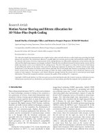
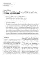
We show the bit error rate (BER) versus the signal-to-
noise ratio (snr)for3usersinFigure 1(a) and 16 users
in Figure 1(b) with 512 training symbols. The solution is
almost linear and all the receivers perform similarly well
except for the nonlinear SVM for 16 users. The training
sequence for the nonlinear SVM with 16 users is not long
enough, and hence the nonlinear SVM is unable to detect
the transmitted bits and reports chance-level performances.
The GPR solution is quite similar to the MMSE solution,
because it almost shuts down its nonlinear part in (28). As we
show in Section 3, the GPR with a linear kernel and the linear
MMSE provide equivalent solutions in this case. This result
is quite relevant, as we do not tell the GPR receiver that the
solution is linear. It finds out on its own, when it maximizes
the hyperparameters’ likelihood. The GPC also cancels its
nonlinear part and it is able to avoid overfitting. The linear
SVM detector presents the worse performance among the
proposed methods that converge in both cases, although it
is barely noticeable in the figures.
The optimal solution is almost linear and all the pro-
posed procedures perform equally well, once the training

sequence is long enough. The training sequence of 512
symbols is not long enough for the nonlinear SVM with
16 users and it is unable to correctly tune its multiuser
detector. If we had increased the training sequence to several
thousand samples, the nonlinear SVM would converge and
it would provide a solution close to the other algorithms.
The differences in BER are not significant to decide which
method is best, but the differences in training time might
lead us to choose one over the others, as we discuss in short.
n = 512
10
−6
10
−5
10
−4
10
−3
10
−2
10
−1
10
0
BER
0 2 4 6 8 10 12 14
snr
(a)
n = 512
10

−6
10
−5
10
−4
10
−3
10
−2
10
−1
10
0
BER
2 4 6 8 10 12 14 16 18
snr
MMSE
GPR
GPC
SVMl
SVMnl
(b)
Figure 1: We report the BER versus the snr foramultiuserdetector
with 3 users in (a) and 16 users in (b). The dashed line represents
the linear MMSE receiver, the solid line the GPR, the dash-dotted
line the GPC, the dotted line with circles the linear SVM, and the
dotted line with bullets the nonlinear SVM.
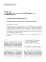
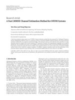
We report the BER as a function of the training examples
for3usersinFigure 2(a) and 16 users in Figure 2(b). For this
experiment, these results are more meaningful than the BER

versus snr reported in Figure 1, because there is a significant
disparity between the performances of the different methods.
For 3 users (Figure 2(a)), the GPR and linear SVM are
able to reduce the BER for very short-training sequences
while GPC, MMSE, and nonlinear SVM need substantially
longer training sequences before they provide nonchance-
level performances. For 32 training symbols, there are 3
orders of magnitude difference in BER between the former
and latter methods.
8 EURASIP Journal on Advances in Signal Processing
snr = 14 dB
10
−6
10
−5
10
−4
10
−3
10
−2
10
−1
10
0
BER
3456789
log
2
n

(a)
snr = 18 dB
10
−7
10
−6
10
−5
10
−4
10
−3
10
−2
10
−1
10
0
BER
3456789
log
2
n
MMSE
GPR
GPC
SVMl
SVMnl
(b)
Figure 2: We report the BER versus the length of the training

sequence for a multiuser detector with 3 users and snr
= 14 dB in
(a) and 16 users and snr
= 18 dB in (b). The dashed line represents
the linear MMSE receiver, the solid line the GPR, the dash-dotted
line the GPC, the dotted line with circles the linear SVM, and the
dotted line with bullets the nonlinear SVM.
From these 2 plots, we can easily understand why the
nonlinear SVM is unable to converge for 16 users with 512
training symbols. For 3 users, the nonlinear SVM needs
longer training sequences than the other methods, before it
can significantly reduce the BER. For 16 users, the learning
problem is harder and it needs several thousand samples to
achieve convergence.
The GPR, MMSE, and linear SVM learn the solution
as the number of training examples increases and they
behave almost equally well for 16 users. The GPC needs the
training sequence to be long enough before it can produce
a meaningful solution. It needs at least 64 symbols for 3
users and 256 for 16 to be able to produce nonchance-
level performances. But once the training sequence is long
enough, it converges to the optimal solution. It does not
provide intermediate solutions as the other methods do.
For 16 users, the GPR receiver presents the fastest
learning curve closely followed by the linear MMSE and
linear SVM solutions. We conjecture this is due to the GPR
optimal training of its hyperparameter, because it is able
to adjust them for each training sequence, while the linear
SVM uses a constant setting, which might be good for a long
training sequence, but not as good for shorter ones.

In this example, we can readily understand the advan-
tages of using GPR for solving multiuser detection problems,
as for very short-training sequences, we are able to obtain
the best possible solution, and if it is linear, it even improves
the linear MMSE solution. The GPR and linear MMSE
detectors provide the same solution as the number of samples
increases; but for short-training sequence, the GPR detector
is able to optimally set its hyperparameters to provide better
performance than the linear MMSE. Also, as we see in the
next example, if the solution is nonlinear, it is able to achieve
nonlinear multiuser detectors, significantly improving the
linear MMSE solution.
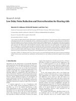
6.2. Nonlinear multiuser detection
We repeat Experiment 2 in [22], in which 3 users transmit
with an orthogonal 8-dimension spreading code. The solu-
tion for user 2 is highly nonlinear and we report the BER
versus the snr in Figure 3. The linear SVM and MMSE clearly
underperform compared to the nonlinear methods. The
GPR and nonlinear SVM achieve almost identical results.
The GPC for low snr mimics the results of the nonlinear
methods (snr < 14 dB); and for high snr, it reports the same
results as the linear receivers (snr > 16 dB). This behavior
is explained by the length and diversity of the training
sequence. If the training sequence is long enough, the
GPC receiver provides the best nonlinear decision function,
otherwise it reports the best linear decision function to avoid
overfitting. For low snr, 512 symbols is long enough for the
GPC to achieve the best nonlinear decision function and
the GPC receiver trains its hyperparameters to obtain this
nonlinear detector. For high snr, there is not enough diversity

in a training sequence with 512 symbols and it is only able to
report the best linear detector, as it shuts down its nonlinear
part to avoid overfitting. In the first experiment, we already
saw that GPC receivers need longer training sequences than
GPR, even to achieve the best linear detector. It is clear in
this experiment that for nonlinear decision function, GPC
receivers even need longer training sequences.
In these two experiments, we are able to show that the
GPR with the covariance function in (28)isabletoobtain
the best results in both scenarios. If the solution is linear,
it performs as the linear MMSE, needing shorter-training
sequences. If the solution is nonlinear, the GPC receiver
builds a nonlinear detector that significantly improves the
F. P
´
erez-Cruz and J. J. Murillo-Fuentes 9
n = 512
10
−7
10
−6
10
−5
10
−4
10
−3
10
−2
10

−1
10
0
BER
24681012141618
snr
MMSE
GPR
GPC
SVMl
SVMnl
Figure 3: We report the BER versus snr foramultiuserdetector
with 3 users and a training sequence of 512 symbols. The dashed
line represents the linear MMSE receiver, the solid line the GPR,
the dash-dotted line the GPC, the dotted line with circles the linear
SVM and the dotted line with bullets the nonlinear SVM. The linear
SVM is on top of the linear MMSE line.
linear MMSE and reports the same solution as a nonlinear
SVM. The nonlinear SVM is not as good as the GPR with
the covariance matrix in (28), because for (almost) linear
solutions, it needs significantly longer training sequences,
which is a waste of resources in wireless communication
systems, as the preamble must be as short as possible. Also
a SVM cannot use a kernel as in (28), because it would need
to cross validate (or hand pick) too many hyperparameters.
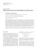
6.3. Nonlinear channel equalization
Now we turn to the channel equalization problem, in which
the channel is represented by (33), and we add a memoryless
nonlinearity to the receiver that transforms each received
signal as follows:

x
i
= x
i
+0.2x
2
i
−0.1x
3
i
+ z
i
, (34)
where
x
i
= (Hs)
i
. This channel model is typically used to
described nonlinear amplifiers in wireless communication
receivers as explained in [12]. To construct the equalizers, we
use 6 received samples to predict each transmitted symbol
with a delay of 2 samples.
In Figure 4, we show the BER versus the snr for all
equalizers and n
= 512. For snr less than 22 dB, the nonlinear
GPR equalizer achieves the minimum BER with a gain
larger than 3 dB for BER around 10
−3
.Forlargersnr, the

performance of this nonlinear equalizer degrades and the
linear equalizers perform significantly better. The nonlinear
SVM equalizer performs as the GPR equalizer for snr lower
than 17 dB, but for larger snr the training sequence is not
n = 512
10
−5
10
−4
10
−3
10
−2
10
−1
10
0
BER
0 5 10 15 20 25
snr
MMSE
GPR
GPC
SVMl
SVMnl
Figure 4: We report the BER versus snr for a channel equalization
problem with a nonlinear channel model. The dashed line repre-
sents the linear MMSE receiver, the solid line the GPR, the dash-
dotted line the GPC, the dotted line with circles the linear SVM,
and the dotted line with bullets the nonlinear SVM.

long enough and its solution degrades (overfitting). For snr
larger than 20 dB, the nonlinear SVM equalizer is not able to
reduce the achieved BER. The nonlinear SVM and the GPR
as the snr increases are not able to get optimal equalizers,
because there is not enough diversity in the training sequence
and they overfit to it. The GPR performance is better than
the SVM for large snr, because it uses a covariance function
in (28) that incorporates a linear term. Although it overfits
the nonlinear part, the linear component allows the GPR to
reduce the BER for large snr. If we had increased the training
sequence, the SVM and GPR would perform better than the
linear methods for larger values of the snr.
The GPC shuts down the nonlinear part and performs as
the linear SVM. This is the same effect that we saw for large
snr in Figure 3, the training set is not long enough to ensure
it can train the nonlinear part of its covariance function and
it consequently sets it to zero. In Figure 4 for snr less than
10 dB, although we can barely notice it, the GPC equalizer
follows the nonlinear solutions, as the training sequence is
long enough to train its nonlinear component in this case.
The linear SVM and GPC are able to perform signif-
icantly better than the linear MMSE, because the channel
model is nonlinear. For a nonlinear channel, the received
constellation is no longer symmetric, and penalizing the
squared error is suboptimal, as it forces that all the detected
symbols to be equally far from its optimal value. The SVM
and GPC equalizers only care if the points are correctly
classified and they only focus on those that might not be,
which explains the BER gap between the linear MMSE
equalizer and the GPC and linear SVM ones.

10 EURASIP Journal on Advances in Signal Processing
In any case, for the snr of interests between 10 and 20 dB,
the GPR receivers (and nonlinear SVM) are significantly
better than the linear methods and the GPC. For this
range of snr, the BER is not low enough for most digital
communication applications, but we can significantly reduce
the BER using channel coding strategies [37] with high-data
rates, instead of increasing the snr.
6.4. Discussion
In the experiments, we show the behavior of GPR for
designing digital communication receivers and we show it
has many favorable properties for solving such task when we
use it with the covariance function in (28).
(i) If the solution is linear, the GPR receiver shuts down
the nonlinear part of the covariance function and performs
as the linear MMSE detector for long training sequences.
It converges faster than the MMSE detector to the optimal
solution. It does not degrade its performance when canceling
the nonlinear part of the kernel.
(ii) If the solution is nonlinear, the GPR receiver is able to
achieve very good performances, comparable to a nonlinear
SVM receiver with optimal hyperparameters, and it needs
shorter-training sequences to achieve such solutions. The
GPR receiver performs significantly better than the linear
detectors.
(iii) The GPR receiver performs a single optimization
procedure. This is a highly desirable quality as in one step
we get the optimal hyperparameters without needing to try
several solutions and check which one is best. The GPR
decides if it needs a linear or a nonlinear solution in that

single optimization without relying on a “genie” or another
procedure to check if the optimal solution is linear.
(iv) The GPR can overfit if the training sequence is not
sufficiently long, as we can see in Figure 4. But in this case
the overfitting does not degrade the solution as much as it
does for the nonlinear SVM. It only happens for very large
snr, in which we do not typically transmit.
(v) The GPR receiver uses a least square lost function,
which is not ideal for solving classification problems when
we are interested in minimizing the misclassification error.
But for digital communication problems in which the noise
is Gaussian, the use of this loss function is not critical and
the GPR-receiver performs as well as the receivers based on
classification loss functions (GPC and SVM).
The GPC would initially seem like a better choice
for designing digital communication receivers, because it
minimizes the misclassification error and it can optimize
the hyperparameters, just as the GPR does. But in our
experiments we show that GPC receivers usually need longer
training sequences before they can tune their nonlinear part
and they decide to train a linear detector in cases where
a nonlinear detector clearly performs better. We believe
that in order for GPC to perform better than (as well as)
GPR receivers, we need far longer training sequences, which
might not be available in digital communication systems.
We conjecture that this limitation of GPC for training
digital communication receiver is due to the posterior
approximation, because its loss function is more suitable
than the ones the GPR uses and we train the GPC receiver
with the same covariance function.

The SVM performs as well as GPR for the proposed
problem, but it needs longer training sequence to deal with
its fixed hyperparameters or longer training resources to
fine tune its hyperparameters. We do not believe there is an
intrinsic advantage for GPR for this problem. Although we
believe that GPR being able to tune its hyperparameters by
maximum likelihood allows solving the problem easier, as we
build the receiver with a single optimization procedure.
7. CONCLUSIONS
We have proposed GPR and GPC for designing digital
communication receivers. GPR follows a wide range of
machine learning tools that have been successfully applied
to the design of digital communication receivers. But GPR
presents several properties that we believe make it a much
better candidate for designing these receivers. First of all,
GPR can be viewed as a nonlinear MMSE. MMSE is the
standard criterion used for designing digital communication
receivers, as it trades off inverting the channel and not
amplifying the noise. Second, its solution is analytical
given the nonlinear function, while most machine learning
methods need to perform an optimization problem to
achieve their solution. Third, it can train its hyperparameters
by maximum likelihood, while other machine learning
algorithms need to cross-validate their hyperparameters or
structure. Forth, its computation complexity is not a limiting
issue as addressed in [5].
To highlight the advantages of GPs as digital com-
munications receivers we compare their performances to
that of SVM. SVM provides solutions as good as the GPR
does, but it needs more training samples. The GPR fits

its covariance function by maximum likelihood, and hence
it does not suffer from this problem. The GPC could be
initially thought of as a better candidate for designing digital
communication receivers, since we are solving a classification
problem. However, as we have shown in this paper it needs
significantly longer training sequences to provide the same
accuracy level as GPR receivers. One possible advantage of
GPC compared to GPR for digital communication receivers
is that they provide posterior probability estimates for the
received bits, which could be sequentially used by a channel
decoder to improve the BER. Some preliminary results of this
idea can be found in [39].
ACKNOWLEDGMENTS
This work was partially funded by the Spanish government
(Ministerio de Educaci
´
on y Ciencia TEC2006-13514-C02-
01/TCM and TEC2006-13514-C02-02/TCM), the European
Union (FEDER), and the Comunidad de Madrid (project
“PRO-MULTIDIS-CM,” id. S0505/TIC/0223). Fernando
P
´
erez-Cruz is supported by Marie Curie Fellowship 040883-
AI-COM.
F. P
´
erez-Cruz and J. J. Murillo-Fuentes 11
REFERENCES
[1] M. Salehi and J. G. Proakis, Communication Syste ms Engineer-
ing, Prentice-Hall, New York, NY, USA, 2nd edition, 2001.

[2] A. O’Hagan and J. F. C. Kingman, “Curve fitting and optimal
design for prediction,” Journal of the Royal Statistical Society
Series B, vol. 40, no. 1, pp. 1–42, 1978.
[3] C. K. I. Williams and C. E. Rasmussen, “Gaussian processes
for regression,” in Advances in Neural Information Processing
Systems,D.S.Touretzky,M.C.Mozer,andM.E.Hasselmo,
Eds., vol. 8, pp. 514–520, MIT Press, Cambridge, Mass, USA,
1996.
[4] C. E. Rasmussen and C. K. I. Williams, Gaussian Processes for
Machine Learning, MIT Press, Cambridge, Mass, USA, 2006.
[5] J. Qui
˜
nonero-Candela and C. E. Rasmussen, “A unifying
view of sparse approximate Gaussian process regression,” The
Journal of Machine Learning Research, vol. 6, no. 2, pp. 1939–
1960, 2005.
[6] G. J. Gibson, S. Siu, and C. F. N. Cowan, “The application of
nonlinear structures to the reconstruction of binary signals,”
IEEE Transactions on Signal Processing, vol. 39, no. 8, pp. 1877–
1884, 1991.
[7]S.Chen,G.J.Gibson,C.F.N.Cowan,andP.M.Grant,
“Reconstruction of binary signals using an adaptive radial-
basis-function equalizer,” Signal Processing,vol.22,no.1,pp.
77–93, 1991.
[8]J.Cid-Sueiro,A.Art
´
es-Rodr
´
ıguez, and A. R. Figueiras-Vidal,
“Recurrent radial basis function networks for optimal symbol-

by-symbol equalization,” Signal Processing, vol. 40, no. 1, pp.
53–63, 1994.
[9] T.Kohonen,K.Raivio,O.Simula,O.Venta,andJ.Henriksson,
“Combining linear equalization and self-organizing adap-
tation in dynamic discrete-signal detection,” in Proceedings
of the International Joint Conference on Neural Networks
(IJCNN ’90), vol. 1, pp. 223–228, San Diego, Calif, USA, June
1990.
[10] P R. Chang and B C. Wang, “Adaptive decision feedback
equalization for digital satellite channels using multilayer
neural networks,” IEEE Journal on Selected Areas in Commu-
nications, vol. 13, no. 2, pp. 316–324, 1995.
[11] F. J. Gonz
´
alez-Serrano, F. P
´
erez-Cruz, and A. Art
´
es-Rodr
´
ıguez,
“Reduced-complexity equaliser for nonlinear channels,” Elec-
tronics Letters, vol. 34, no. 9, pp. 856–858, 1998.
[12] B. Mitchinson and R. F. Harrison, “Digital communications
channel equalization using the Kernel Adaline,” IEEE Transac-
tions on Communications, vol. 50, no. 4, pp. 571–576, 2002.
[13] F. P
´
erez-Cruz,
´

A. Navia-V
´
azquez, P. L. Alarc
´
on-Diana, and
A. Art
´
es-Rodr
´
ıguez, “SVC-based equalizer for burst TDMA
transmissions,” Signal Processing, vol. 81, no. 8, pp. 1681–1693,
2001.
[14] D. G. M. Cruickshank, “Radial basis function receivers for DS-
CDMA,” Electronics Letters, vol. 32, no. 3, pp. 188–190, 1996.
[15] R. Tanner and D. G. M. Cruickshank, “Volterra based receivers
for DS-CDMA,” in Proceedings of the 8th IEEE International
Symposium on Personal, Indoor and Mobile Radio Communi-
cations (PIMRC ’97), vol. 3, pp. 1166–1170, Helsinki, Finland,
September 1997.
[16] M. S
´
anchez-Fern
´
andez, M. de-Prado-Cumplido, J. Arenas-
Garc
´
ıa, and F. P
´
erez-Cruz, “SVM multiregression for non-
linear channel estimation in multiple-input multiple-output

systems,” IEEE Transactions on Signal Processing, vol. 52, no. 8,
pp. 2298–2307, 2004.
[17] M. Mart
´
ınez-Ram
´
on, J. L. Rojo-
´
Alvarez, G. Camps-Valls, and
C. G. Christodoulou, “Kernel antenna array processing,” IEEE
Transactions on Antennas and Propagation,vol.55,no.3,pp.
642–650, 2007.
[18] F J. Gonz
´
alez-Serrano, J. J. Murillo-Fuentes, and A. Art
´
es-
Rodr
´
ıguez, “GCMAC-Based predistortion for digital modula-
tions,” IEEE Transactions on Communications,vol.49,no.9,
pp. 1679–1689, 2001.
[19] J. Arenas-Garc
´
ıa, M. Mart
´
ınez-Ram
´
on,
´

A. Navia-V
´
azquez,
and A. R. Figueiras-Vidal, “Plant identification via adaptive
combination of transversal filters,” Signal Processing, vol. 86,
no. 9, pp. 2430–2438, 2006.
[20] G. S. Kimeldorf and G. Wahba, “Some results in Tchebychef-
fian spline functions,” Journal of Mathematical Analysis and
Applications, vol. 33, no. 1, pp. 82–95, 1971.
[21] C. M. Bishop, Neural Networks for Pattern Recognition,
Clarendon Press, Oxford, UK, 1995.
[22] S. Chen, A. K. Samingan, and L. Hanzo, “Support vector
machine multiuser receiver for DS-CDMA signals in multi-
path channels,” IEEE Transactions on Neural Networks, vol. 12,
no. 3, pp. 604–611, 2001.
[23] J. J. Murillo-Fuentes, S. Caro, and F. P
´
erez-Cruz, “Gaussian
processes for multiuser detection in CDMA receivers,” in
Advances in Neural Information Processing Systems, Y. Weiss, B.
Sch
¨
olkopf, and J. Platt, Eds., vol. 18, pp. 939–946, MIT Press,
Cambridge, Mass, USA, 2006.
[24] F. P
´
erez-Cruz and J. J. Murillo-Fuentes, “Gaussian processes
for digital communications,” in Proceedings of the IEEE Inter-
national Conference on Acoustics, Speech and Signal Processing
(ICASSP ’06), vol. 5, pp. 781–784, Toulouse, France, May

2006.
[25] S. Caro, F. P
´
erez-Cruz, and J. J. Murillo-Fuentes, “Gaussian
processes for regression in channel equalization,” in Pro-
ceedings of the 14th European Signal Processing Conference
(EUSIPCO ’06), Florence, Italy, September 2006.
[26] C. K. I. Williams and D. Barber, “Bayesian classification with
Gaussian processes,”
IEEE Transactions on Pattern Analysis and
Machine Intelligence, vol. 20, no. 12, pp. 1342–1351, 1998.
[27] M. Kuss and C. E. Rasmussen, “Assessing approximate infer-
ence for binary Gaussian process classification,” The Journal of
Machine Learning Research, vol. 6, pp. 1679–1704, 2005.
[28] T. M. Cover and J. A. Thomas, Elements of Information Theory,
John Wiley & Sons, New York, NY, USA, 1991.
[29] G. G. Raleigh and J. M. Cioffi, “Spatio-temporal coding for
wireless communication,” IEEE Transactions on Communica-
tions, vol. 46, no. 3, pp. 357–366, 1998.
[30] R. Parisi, E. D. Di Claudio, G. Orlandi, and B. D. Rao, “Fast
adaptive digital equalization by recurrent neural networks,”
IEEE Transactions on Signal Processing, vol. 45, no. 11, pp.
2731–2739, 1997.
[31] V. N. Vapnik, Statistical Learning Theory,JohnWiley&Sons,
New York, NY, USA, 1998.
[32] B. Sch
¨
olkopf and A. Smola, Learning with Kernels, MIT Press,
Cambridge, Mass, USA, 2001.
[33] F. P

´
erez-Cruz and O. Bousquet, “Kernel methods and their
potential use in signal processing,” IEEE Signal Processing
Magazine, vol. 21, no. 3, pp. 57–65, 2004.
[34] C. K. I. Williams, “Prediction with Gaussian process: from
linear regression to linear prediction and beyond,” in Learning
in Graphical Models, M. I. Jordan, Ed., pp. 599–621, MIT Press,
Cambridge, Mass, USA, 1999.
12 EURASIP Journal on Advances in Signal Processing
[35] S. Haykin, Neural Networks: A Comprehensive Foundation,
Prentice-Hall, Upper Saddle River, NJ, USA, 2nd edition, 1999.
[36] L. L. Scharf, Statistical Signal Processing: Detection, Estimation,
and Time Series Analysis, Addison-Wesley, New York, NY,
USA, 1990.
[37] D. J. C. MacKay, Information Theory, Inference and Learning
Algorithms, Cambridge University Press, Cambridge, UK,
2003.
[38] R. Gold, “Optimal binary sequences for spread spectrum
multiplexing,” IEEE Transactions on Information Theory, vol.
13, no. 4, pp. 619–621, 1967.
[39] F. P
´
erez-Cruz, P. Mart
´
ınez-Olmos, and J. J. Murillo-Fuentes,
“Accurate posterior probability estimates for channel equaliza-
tion using Gaussian processes for classification,” in Proceedings
of the IEEE 8th Workshop on Signal Processing Advances in
Wireless Communications (SPAWC ’07), pp. 1–5, Helsinki,
Finland, June 2007.