Quantitative Techniques for Competition and Antitrust Analysis_8 docx

7.1. Quantifying Damages of a Cartel 373
Q
P, c
S'
S
P
Inelastic
P
Elastic
Demand
Elastic
Demand
Inelastic
P
0
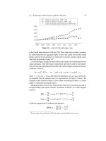
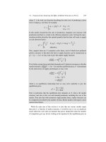
Figure 7.8. Pass-on with elastic and inelastic demand.
For a formal demonstration, consider a price-taking firm, solving
max
q
pq  C.qIc/;
where C.qIc/ represents the total cost function and c represents a cost driver. From
this problem we derive the firm supply function q D s.p; c/ and from that in turn,
given N identical firms, we derive an industry supply curve S.pIc/, increasing in
p and decreasing in c. We may now define a function
F.pIc/ Á D.p/  S.pIc/ D 0;
which implicitly defines the equilibrium price as a function of our cost driver, c.
We can then apply the Implicit Function Theorem to get an expression for the
pass-through @p=@c. Specifically, totally differentiating gives
@D.p/
@p
D

@S.pIc/
@p
C
@S.pIc/
@c
@c
@p
;
which in turn suggests that when the downstream market is perfectly competitive
the pass-on effect can be expressed as
@p
@c
D
@S.pIc/
@c
Â
@D.p/
@p

@S.pIc/
@p
Ã
D
Â

@ ln S.pIc/
@c
ÃÂ

@ ln D.p/

@p
C
@ ln S.pIc/
@p
Ã
;
where the latter equality follows by noting first that D.p/ D S.pIc/, second that
for any nonzero differentiable function f.p/we can write
@ ln f.p/
@p
D
1
f.p/
@f .p/
@p
374 7. Damage Estimation
and thirdly by multiplying top and bottom by minus one. Finally, note that (i) the
demand elasticity is negative while the supplyelasticityis positive so that the denom-
inator will be positive and (ii) supply will decline as costs increase so that the numer-
ator is also positive, making the ratio positive so that equilibrium prices increase
with cost, @p=@c > 0. Furthermore, we conclude that the pass-on depends on both
the demand and supply elasticities as well as on the cost elasticity of supply. Both
elastic demand or elastic supply make the denominator large and hence reduce the
pass-through down toward zero. Similarly, and intuitively, when the cost elasticity of
supply is small so that costs tend not to impact on ability to supply the downstream
good, the rate of pass-through will be small.
Verboven and Van Dijk (2007) derive the analytical formulas for the pass-on rate
under perfectly competitive markets and under markets with oligopolistic competi-
tion. Furthermore, they evaluate the relative importance of the pass-on and output
effects for a variety of settings. They note that the pass-on effect should be applied

and the amount of the overcharge discounted by this effect when the claimant oper-
ates in a fully competitive setting. But when the claimant’s industry—the down-
stream industry—is less competitive, the output effect and the loss of sales volume
by the claimant starts mitigating the effect of the pass-on on the claimants profits.
The output effect should in such cases limit the discount in the damages granted by
a pass-on defense. Their paper provides analytical expressions for the total discount
to be applied to the overcharge of the cartel, taking into account both the pass-on
and the output effects.
Cournot competition in quantities the pricing function has the form
P.Q/CP
0
.Q/q D mc;
which under firm symmetry implies
P.Q/CP
0
.Q/
Q
N
D mc
or
1 C
1
NÁ.Q/
D
mc
P.Q/
;
where Á is the price elasticity of demand,
Á.Q/ Á
@ ln P.Q/

@Q
D
1
P.Q/
@P .Q/
@Q
:
This equation defines implicitly our equilibrium output
F.Q;mc/ Á 1 C
1
NÁ.Q/

mc
P.Q/
D 0;
7.1. Quantifying Damages of a Cartel 375
which in turn means, given the demand equation, we can calculate the implied level
of prices since the inverse demand curve describes p D P.Q/. First, recall that if
p D P .Q.mc//, then
@p
@mc
D
@P .Q/
@Q
@Q.mc/
@mc
;
where the former is just a property of the inverse demand equation and the latter we
can calculate by applying the implicit function theorem to the Cournot equilibrium
equation:

F.Q;mc/ D 0:
Noting that
13
@F .Q; mc/
@Q
Á
1
N.Á.Q//
2
@Á.Q/
@Q
C
mc
P.Q/
2
@P .Q/
@Q
and
@F .Q; mc/
@mc
Á
1
P.Q/
;
we can apply the implicit function theorem by noting that
@Q.mc/
@mc
D
Â
@F .Q; mc/

@mc
ÃÂ
@F .Q; mc/
@Q
Ã
1
and hence, given the results above, that
@p
@mc
D
@P .Q/
@Q
@Q.mc/
@mc
D
@P .Q/
@Q
Â
1
P.Q/
ÃÂ

1
N.Á.Q//
2
@Á.Q/
@Q
C
mc
.P .Q//

2
@P .Q/
@Q
Ã
:
Rearranging gives
@p
@mc
D
@P .Q/
@Q
@Q.mc/
@mc
D
@ ln P.Q/
@Q
Â
1
N.Á.Q//
@ ln Á.Q/
@Q

mc
P.Q/
@ ln P.Q/
@Q
Ã
1
()
so that canceling terms gives

@p
@mc
D
Â
Q
N
@ ln Á.Q/
@Q

mc
P.Q/
1
Q
Ã
1
;
where Á is the price elasticity of demand. Note that in the Cournot model the sensi-
tivity of the price elasticity of demand to the output level affects the pass-through.
The expression does not allow us to predict whether the pass-on under Cournot will
be lower or higher than under perfect competition.
376 7. Damage Estimation
7.1.4 Timing the Cartel
An area we have not yet considered is the timing of the cartel. We need to understand
the time when the cartel was active since damages will accrue over that period. In
fact, getting the periodsufficiently approximately correct maybe at least as important
for the final damages number as pinning down exactly what the difference between
collusive and competitive prices would have been in any given time period. In
addition, most methodologies rely at least to some extent on pre-cartel or post-
cartel data to extract information about the competitive scenario and it is therefore
rather important that the data deemed to be the result of competition are in fact

genuinely the result of competition, or something very close to it.
Most commonly investigators use direct data from company executives to time
the cartel: notes from diaries, records of meetings, emails referring to meetings or
exchange of information, and memos describing pricing schemes. All these are the
best sources for timing the cartel, as well as proving it existed in the first place.
Because they are generally simple and less controversial pieces of evidence, it is
by far the preferred source of information. Such information may be obtained from
raiding company offices or executives’home addresses.Alternatively, it may emerge
from the now widespread use of leniency programs, where leniency (particularly
for second and subsequent leniency applications in a given case) can sometimes be
conditional on providing evidence about the workings of a cartel.
However, if there is not enough hard documentary evidence to time the cartel
precisely, investigators may want to consider looking for a structural break in the
data. The idea is to look for a change in the competition regime prevailing in the
industry and the intuition is that we expect changes in conduct to be associated with
otherwise unexplained changes in the levels of prices and/or quantities being sold.
One way to do this is to specify dummy variables that allow for multiple possible
starting and finishing dates. For instance, one might run the following regression:
p
t
D x
0
t
ˇ C˛
1
D
April 06 to May 06
t
C ˛
2

D
June 06 to July 06
t
C "
t
:
This specification nests two timing options with two different starting dates. If
˛
1
D 0 and ˛
2
>0, then the starting date of the cartel is June 2006. If ˛
1
D ˛
2
>0,
then the starting date of the cartel is April 2006.
One can undertake a similar exercise for the end dates of the cartel but end dates
are often trickier to pin down than start dates. Reversion to competition can be a
gradual process and is not always marked by a discrete event such as a meeting
among executives. Cartels often collapse little by little due to cheating, entry, a
diversion of interests, or due to scrutiny by a competition authority. One may observe
prices falling with several attempts to re-establish coordination having some limited
success. Documenting and incorporating these data into the analysis may not be
straightforward.
7.2. Quantifying Damages in Abuse of Dominant Position Cases 377
Additionally, there are reasons to think that the cartel may be replaced by a
competition regime that is not necessarily genuine competition. The fact that a
cartel had explicitly solved the problem of agreeing what it meant to be colluding
meant that the first of Stigler’s conditions for tacit collusion may be satisfied, namely

agreement (see the discussion in chapter 6). There are numerous indications that tacit
collusion may be more likely after periods of explicit collusion and examples that are
widely cited include those which followed the breakdown of the electrical cartels in
the late 1950s.
14
Alternatively, firms in the previously cartelized industry which are
being exposed to damage claims may sometimes have an incentive to price above
the noncollusive level in the post-cartel period in order to minimize the size of their
penalty (Harrington 2003).
Finally, it is worth noting that the focus on claims made by downstream firms in
the discussion of cartel damages reflects, in part, a legal reality, at least in Europe.
The fact is that groups of final consumers often find it very difficult to coordinate
together to generate a successful damages claim. Legal fees in a damages case can
be substantial, even if a regulator has already put together a civil case establishing
there was a cartel, while each consumer’s damage may be small. For example, in the
football shirt case in the United Kingdom (JJB Sports) that consumer organization
Which? took to the Competition Appeals Tribunal on behalf of consumers, each
consumer was awarded £20 in damages from the company. However, since in the
United Kingdom this kind of private action requires consumers to opt into the group
of consumers that were represented byWhich?, only approximately1,000 consumers
were expected to receive £20 each in compensation while almost one million shirts
were estimated to have been affected by the cartel.
15
The possibility for a limited
form of U.S style class-action suits, where groups of consumers would need to
opt out of an action rather than opt into it, is under consideration in a number of
European jurisdictions.
16
7.2 Quantifying Damages in Abuse of Dominant Position Cases
Damages are mostly explicitly calculated for cartel infringements. However, monop-

olization cases (or in EU language abuse of a dominant position cases) may also
harm the process of competition and ultimately consumers. Because the tradition of
14
Specifically, the General Electric–Westinghouse case provides an example where it was subsequently
alleged that tacit collusion replaced the explicit collusion of the late 1950s (see Porter 1980).
15
See, for example, “Thousands of football fans win ‘rip-off’ replica shirt refunds” (http://business.
timesonline.co.uk/tol/business/law/article3159958.ece). The other aspect of the incentive to take such
cases on behalf of consumers is the allocation of costs. If a case is won by a consumer organization, it
can seek its costs; however, this “loser-pays” principle puts a considerable risk of a large downside on
consumer organizations if the court decides that a claim for damages is without merit.
16
See www.oft.gov.uk/news/press/2007/63-07 for the United Kingdom and />competition/antitrust/actionsdamages/index.html for the European Commission’s consultation on private
actions.
378 7. Damage Estimation
private litigation is not yet fully developed in Europe, there are not many examples
of calculated damages for individual misconduct unrelated to price fixing. This sec-
tion only briefly introduces the topic and draws from Hall and Lazear (1994) and
the Ashurst (2004) study for the European Commission.
7.2.1 Lost Profits
Abuses of dominant position hurt consumers directly through exploitative abuses
(high prices)but additional harm toconsumers often also occurs because competition
has been impaired in some way. For example, rivals have been prevented from
operating in the market either entirely or perhaps their scale of operation has been
reduced. In either case, we will say they have suffered from an exclusionary abuse.
Who, if anybody at all, is entitled to claim damages is a matter of law and differs
by jurisdiction.
The calculation of damages arising from an abuse of dominant position is a fairly
uncommon activity for competition authorities, far rarer than damage calculations
are for cartels. One reason may be that the damage inflicted by a dominant firm on

customers and the extra profits generated by the abusive conduct can be very difficult
to calculate whenever there is a significant element of exclusionary abuse. Indeed,
there are few well-understood methodologies for evaluating the damage caused by
exclusionary abuses, although a simulation model could be used in principle. By
its very nature estimating what competition would have been like with additional
firms active is a very difficult exercise. The quantification of the additional profits
generated by the abuse, on the other hand, may be of interest if the authority wants
to assess the incentives that firms face for engaging in abusive behavior of some
kind. The methods presented here could also be used for such a purpose.
When the injured party is a rival and not a customer, the damage calculation is even
less straightforward. Typically, damages will be expressed as the additional profits
that would have been obtained if the abuse had never taken place. The counterfactual
is more difficult to establish than the effect on consumers since it will involve the
performance of a particular firm if it had faced different conditions on the market.
While our current generation of simulation models might be used to incorporate
individual abusive conduct and to produce comparative static results of outcomes
with andwithout the conduct, the data required toundertake suchan exercise robustly
would quite possibly rarely be available.
The design of a counterfactual and the quantification of the profit differential
with and without the conduct is the most essential and also the trickiest part of
such a damage estimation exercise. There are, however, other empirical issues that
will also be relevant. For example, if plaintiffs can recover interest from their past
losses, there will have to be a calculation of the present value of past damages.
Similarly, future losses due to irreparable damage will have to be divided by a
suitable discount rate in order to be expressed in net present value. The choice of the
7.2. Quantifying Damages in Abuse of Dominant Position Cases 379
interest rate and the discount factor theoretically appropriate will take into account
the characteristics of the firm and the risk of the investment. While such general
statements are widely acknowledged to be standard practice, they are not the same
as stating the right number for any given context. Doing so with any confidence

would require a substantial endeavor. Finally, the timing of injury may not coincide
with timing of the infringement since injury can extend beyond the infringement and
the claimant may not have been directly affected by the abuse since it took place.
7.2.2 Valuation of Lost Profits
The quantification of lost profits due to an abuse of dominant position by another firm
may well mostly involve using accounting data and accounting concepts to construct
the profitability that would have occurred in the counterfactual world where no
abuse took place. One approach is to base the damage calculations on the claimant
company’s earnings: the damages will be the discounted estimated change in the
cash flow. The cash flow is defined as the firm’s earnings actually received minus
the costs actually incurred. The calculation of cash flow would exclude depreciation
since the cost of depreciation is not actually paid. Assumptions must be made about
how costs would have changed with different output and revenues. The calculation
of “but for” cash flow will have to be carefully based on information about the
company situation before the injury and its likely prospects on the market. The
latter, in particular, means that a sufficiently deep knowledge of the firm and industry
is required for such an exercise, and/or at least a willingness to make reasonable
assumptions.
A second approach to evaluating lost profits is to use a market-based approach.
Damages could be estimated by calculating the loss of sales due to injury and
multiplying that by the stock market valuation of a similar company as a multiple
of its sales. If a similar company’s stock price implies a valuation of double the
sales revenues, the damage to lost sales will be double. This approach eliminates the
need to discount the loss in profits over time but the calculation of the loss in sales
raises the same issues as the calculation of the “but for” cash-flow or the “but for”
scenario in general.A related assets-based approach would calculate the damages as
the change in the book value of assets before and after the infringement. Of course,
for such an approach to be a sensible one, the analyst must be confident that the
change in asset valuation is a consequence of the abuse and reflects the value of
damage.

Each of these techniques has advantages and disadvantages and they all raise the
challenge of constructing a credible “but for” world. Case handlers may have to draw
on the knowledge and industry expertise of an array of professionals such as indus-
try experts, accountants, and strategy managers in order to construct a reasonable
estimate of such damages.
380 7. Damage Estimation
7.3 Conclusions
 Cartels increase prices and diminish output causing both a loss in total welfare
and also a transfer of welfare from customers to producers. Profits go up
and consumer surplus will generally go down under a cartel relative to a
competitive market.
 The total harm caused by a cartel to its customers consists of a direct effect
on the customers who buy from the cartel in the form of an increase in prices
and also an indirect effect due to the restriction in output on those customers
who decide not to buy from a cartel given its high prices. If the cartel sells
an input to downstream firms who then sell on to final consumers, damages
to the downstream firm may be mitigated by the downstream firm’s ability to
pass on the increase in its costs to final consumers.
 In practice, cartel damages are often approximated by the direct damage or
the total amount of the overcharge to the customers. This is the increase in
price times the actual quantity sold during the cartel period.
 Quantifying the damages will require estimating the price that would have
prevailed absent the cartel. When market conditions do not vary greatly, this
can be done by looking at historical time series and taking the price of the com-
petitive periods as the benchmark competitive price during the cartel period.
If market conditions do vary over time, one may nonetheless be able to use a
regression framework to predict the “but for” prices during the cartel period.
Structural simulations of the market are also possible but require reasonable
assumptions on the nature of demand and the type of competition that would
prevail absent the cartel.

 Using the trend in the prices of a similar product to infer the price in the
cartelized market is also possible, assuming such a benchmark is available.
Applying a “reasonable” margin to the cost of the cartelized industry during
the cartel can also provide a “but for” price when such “reasonable” margin
can be inferred from the industry history or other benchmark markets.
 Timing the cartel is a necessary part of damage estimation. It is best done
using documentary evidence but evidence of unexplained structural breaks in
the pricing patterns can sometimes also provide useful guidance.
 The treatment of the pass-on effect in the calculation of damages depends on
the legal framework. The extent of the pass-on will depend on the sensitivity
of the firm’s supply function to the change in costs and also on the demand
and supply elasticities that it faces. When the output effect is very large, so
that a downstream firm’s profits suffer as they lose the margins that would
have been earned on competitive volumes, the ability to pass on cost increases
may not successfully mitigate the damage suffered by the downstream firm.
7.3. Conclusions 381
 In addition to the difficulties in cartel cases, the exercise of quantifying dam-
ages in cases of abuse of dominant position (attempted monopolization) is
further complicated by the difficulty in defining the “but for” world. Dynamic
and strategic elements which are difficult to incorporate might be particularly
relevant in such settings. For example, suppose a claim for damages were
made following the EU’s case against Microsoft for abuse of dominance. To
evaluate the damages suffered by rival firms, we may need to take a view
on the counterfactual evolution of the computer industry—by any measure a
nontrivial task.
8
Merger Simulation
Simulating markets in order to predict the unilateral effect of mergers on prices
has seen considerable growth in popularity since the method was refined during
the 1990s in a series of papers including the famous papers by Farrell and Shapiro

(1990), Werden and Froeb (1993b), and Hausman et al. (1994). Such exercises,
called merger simulations, are used for two purposes. First, they can serve as a
screening device. In that case a standard model is usually taken as an admittedly
very rough approximation to the world withthe expectation that the merger simulated
with that model provides at least as good a screen as the use of market shares or
concentration indices alone and hence is a complementary assessment tool to these
simple methods. The second purpose of merger simulation involves building a more
substantial model with the explicit aim of providing a realistic basis for a “best
guess” prediction of the likely effects of a merger.
Although merger simulation is now familiar to most antitrust economists and has
been applied in a number of investigated cases, authorities remain cautious in the
use of the results of these simulations as evidence. One important reason is that
most authorities’ decisions are subject to review by judges and the courts have not
universally embraced merger simulation as solid probative material. In turn, the
reason for judicial concern is that merger simulation models are based on important
structural assumptions regarding the nature of consumer demand, the nature of
firm behavior, and the structure of costs. Evaluating whether a simulation model
is likely to be accurate therefore implies determining the appropriateness of those
assumptions. Unfortunately, there is usually considerable uncertainty regarding the
price-setting mechanism in the market, the nature of demand, and the nature of costs.
Yet a model builder must make explicit assumptions about each of these important
elements of a merger simulation model.
The alternative empirical approach is to try to use “natural experiments.” In some
cases natural experiments will allow an empirical evaluation with fewer explicit
assumptions. We discussed this important approach in detail in chapter 4. Such
an approach is, however, not always either available or convincing. As a result,
many investigations use a mixture of theoretical arguments, quantitative indicators,
and qualitative descriptions of industry features to decide whether a merger will
lead to a substantial lessening of competition (SLC) causing prices to rise. Such
8.1. Best Practice in Merger Simulation 383

an approach, as the proponents of simulation models point out, will usually not
involve stating explicitly the structural and modeling assumptions on which an SLC
decision is based. Not stating assumptions is clearly not a satisfactory approach
scientifically but it does appear unfortunately to have the legal tactical advantage
that it makes the analysis less prone to challenge. At least, this seems to be the
current state of affairs. At the same time, the appropriate standard of proof for an
investigation should probably not include the requirement to produce a simulation
model of the industry with absolutely realistic assumptions. On many occasions
either peculiar static or dynamic features of a market would make detailed custom-
built simulation modeling extremely difficult. Indeed, such a process may often be
unrealistic on merger inquiry timescales and budgets, particularly when an authority
is investigating relatively small mergers.
Most moderate observers think the bottom line is that a well-designed simulation
model can potentially be very informative and can even in some cases provide a
satisfactory approximation of a merger effect. By integrating the results in a broader
analysis of the qualitative aspects of the industry, merger simulation can provide
further evidence of the effect of mergers on competition. Qualitative and descriptive
analysis can be used to go through the vital task of subjecting any output from a
simulation model, such as predicted prices, to careful scrutiny and “reality checks,”
or at least “sanity checks.”
The uncertainty over exactly the appropriate modeling assumptions has a number
of implications. First, it will mean that one can never claim to have pinned down
with certainty the effect of a merger. Second, it means that measures of uncertainty
calculated under the assumption that the class of models considered includes the
“truth” should probably be treated with appropriate caution.And third, consequently,
it will usually be necessary to at least explore the robustness of the prediction to
deviations in the assumptions made. With these important caveats in mind we turn to
a detailed consideration of simulation models. We present first the general rationale
for merger simulation exercises and a simple illustrative example. We then provide a
more involved discussion going into delving further into the technical complexities.

Finally, we discuss the potential use of merger simulation techniques to assess the
impact of a merger on the incentives to coordinate.
8.1 Best Practice in Merger Simulation
A merger simulation exercise will produce credible results if certain best practices
are followed.
1
Those practices relate to the choice of assumptions, to the data used,
and to the framing of the results within a broader analysis.
Practitioners need to justify their choice of modeling assumptions. It is not enough
to use one of the “standard models” and claim that its widespread use justifies its
1
For a discussion on the assessment of merger simulations, see Werden et al. (2004).
384 8. Merger Simulation
applicability. Instead, one should be able to argue why the theoretical assumptions
are a reasonable approximation of the facts of the case. For example, if firms appear
to compete primarily in advertising rather than prices, then the differentiated prod-
uct Bertrand model may not be a good fit for the industry. Such a situation may be
the case in the music industry, where huge amounts of money are spent promoting
some artists and songs. It would presumably be unwise to focus all of our modeling
attention on the price of the CD or MP3 file, as we would essentially be doing if we
chose a Bertrand pricing model as a description of the way prices are determined
in the industry. Similarly, in industries where we have important technological dif-
fusion effects, static pricing models may well miss important dynamic dimensions
of competition. For example, firms may want to manage diffusion in order to price
discriminate, charging the high-value “first adopters” high prices before moving
price down to service the mass market. Or they may want to accelerate the spread
of the technology by subsidizing the first users. In each case, a simple Bertrand
model would miss the primary economic factors driving economic outcomes in the
industry.
Analogously, in industries where customers really care about the identity of the

producer, be it for quality or institutional reasons, the Cournot model would probably
provide a poor approximation to reality. Other factors that may be important for
the choice of model are the nature of contractual relationships, the identity of the
buyers, the extent of innovation, and the nature of competition either upstream or
downstream. In his commentary on merger simulation models, Walker (2005) notes
how, in defending their Volvo–Scania merger simulation, the expert economists
pointed out that their predicted margins may have been overestimates of the actual
margins because firms may have sold under the equilibrium price to recoup the
lower profits with increased aftermarket sales. Walker argues that if this argument is
correct, then perhaps this pricing behavior should have been captured by the pricing
equation in the model (see also Crooke et al. 1999).And indeed, in building a merger
simulation model investigators need to constantly remind themselves that they are
trying to capture what would actually happen if the proposed change in industry
structure is allowed. The best model may well not be a “standard” one. That said,
there is obviously a limit to the time and resources available to any investigator
and every model anyone has ever built is only an approximation of reality. If the
likely bias in predicted prices can be signed, a simulation model may nonetheless
be informative.
Each of these examples suggests that some simulation exercises, perhaps many,
will require bespoke industry-specific models. If building such models with suffi-
ciently good explanatory power proves intractable within the time available for a
merger inquiry, then it may be that the analysis should rely on careful and informed,
broader, qualitative assessment. Some of the time, however, given enough resources,
it will be possible to construct a model that fits the market sufficiently.
8.1. Best Practice in Merger Simulation 385
If a merger simulation model is built, then the investigator will have to show that
it predicts the facts of the industry reasonably well. In particular, predicted prices,
costs, and margin behavior must be consistent with the reality of the industry. It
is therefore vital to take the time to refine and check the model sufficiently before
proceeding to the merger forecasting exercise. Methods to check the validity of

simulation models include both the use of “in-sample” and “out-of-sample” predic-
tions. Consider, for example, a differentiated products Bertrand model. On the one
hand, checking the fit of the model in terms of predicted prices within sample will
be useful. We may also check “out-of-sample” predictions by estimating the model
on a subset of the data and then using the model to predict prices during the rest
of the sample. However, such direct checks are not usually the end of the matter.
For example, if estimates of price elasticities are wrong, then a Bertrand model will
often produce negative estimates of marginal costs, which obviously cannot be right.
Checking such predictions can provide additional important sanity or possibly even
reality checks.
When the theoretical framework is chosen, parameters need to be estimated or
calibrated. If there are sufficient market data available, econometric estimation may
be possible and good practice for econometric and regression analysis applies. If
there are insufficient data or indeed insufficient time available for estimation and the
model is being used solely as a rough-and-ready screening device, then underlying
parameters may be calibrated using the predicted structural relationships between
observed variables. A poor model will not successfully predict the relationship
between observed variables and, with sufficient attention to validity and checking,
this will usually become very apparent. Of course, the other side of cross checking is
making sure that the data used are representative and correctly measured. In particu-
lar, data on margins, marginal costs, or demand elasticities, which may be retrieved
from industry information, must be checked for consistency and plausibility.
Finally, one should keep in mind that most merger simulations currently involve
static models and do not incorporate dynamic effects. Firms may respond to a merger
by issuing new products, repositioning their current products, or by innovating (see,
for example, Gandhi et al. 2005). Each of these reactions will not be captured by a
merger simulation. If there is a lot of evidencethat the market inquestion has behaved
in the past in a very dynamic fashion and that the competitive environment is subject
to constant change, the merger simulation exercise will certainly lose relevance for
the medium-term prediction of industry outcomes. In those cases,appropriate weight

needs to be given to evidence indicating potential dynamic responses of the market,
although these may well be beyond the usual time horizon of a merger inquiry since
often we expect entry or other competitive responses to at least mitigate the problems
generated by mergers within a few years.
In summary, merger simulation results will usually only be one part of the total
evidence base when evaluating the effects of a merger. Qualitative analysis of the
elements that determine pricing behavior and particularly qualitative analysis of
386 8. Merger Simulation
the aspects of competition not captured by any merger simulation exercise must be
properly incorporated. Only when the model used in the merger simulation fits the
facts on the ground and the prediction of the effects is consistent with the rest of the
evidence, should a merger simulation be used as part of the evidence. Ultimately, the
analyst will want to be solidly aware that judges, rightly, do not like “black boxes”
generating evidence, so every effort must be made to make the analysis clear and
transparent.
The remaining sections in this chapter explain the rationale of merger simulation
using simple and popular models. The purpose is both to outline these popular
options but also to concentrate on the underlying principles that allow investigators
to undertake customized modeling as well as undertake simulations using these
popular modeling choices. There is little doubt that in the future better models
will emerge for a variety of particular circumstances. In addition, better demand
systems and better approaches to cost estimation will be used to generate genuinely
data-driven answers in unilateral effects merger simulation. Experience and a good
understanding of the underlying economics will help the investigating economist
discriminate among the various options and select the appropriate models.
8.2 Introduction to Unilateral Effects
This section will use a simple framework to introduce the economic rationale of
merger simulation and the basic methodological foundations of the exercise. To ease
exposition we will use a familiar framework. Indeed, a major aim of this section is
to put simulation models, which tend to be numerical, into the standard economic

frameworks that are entirely familiar to all professional economists and ubiquitous
tools for analysis. Empirical merger simulation primarily puts those models on a
computer and makes estimates/guesses or “guesstimates” of the parameters of the
models. Along the way we hope to make clear the contribution, assumptions, and
limitations of this approach for analyzing unilateral effects of a merger.
8.2.1 An Introductory Model: Homogeneous Product Cournot
In industries where the product supplied by the firms is homogeneous, firms compete
in quantities with the aim of maximizing profits, and customers do not differentiate
between suppliers, competition can be modeled as a Cournot game. In this setting,
firms choose the quantity of the good that they will produce given the quantity
already supplied by competitors and then offer it at the price determined by aggregate
demand and supply. Firms can affect prices with their output decisions and are
able to raise prices by restricting output or lower them by increasing production.
A merger of undertakings in such a market will have effects that can be easily
described. Farrell and Shapiro (1990) provide a nice discussion of merger analysis
in a Cournot setting. Below, we describe a merger simulation for the very simple
8.2. Introduction to Unilateral Effects 387
case of a duopoly merging to monopoly in a homogeneous product market. The
simplicity of this scenario will help illustrate the concepts involved in an empirical
merger simulation exercise.
8.2.1.1 Mergers in Cournot Industries
In any game theoretic context including Cournot, economists characterize firm
behavior by their best response functions. Consequently, simulating the effect of
a merger involves calculating the best response functions for both the pre-merger
and post-merger scenarios and solving for the corresponding equilibrium prices and
quantities. In the Cournot model, if firms are symmetric in costs, the only differ-
ence between the pre- and post-merger scenarios will be the total number of firms
operating in the market and so this is the variable that will need to be adjusted in the
reaction functions. Symmetry assumptions simplify analysis because, with N play-
ers, N reaction functions arising from a Cournot model become just one equation

to actually solve since all reaction functions are identical. If firms are heteroge-
neous, we will, in general, need to solve for equilibrium quantities by solving all N
reaction functions. We will see this process in action a number of times during this
introductory section.
Whether firms are assumed symmetric or not, we will need an estimate of marginal
cost(s) as well as parameters of the market demand. Once these parameters are
estimated, we can compute the pre-merger quantities and profits using the reaction
functions of a market corresponding to the number of firms existing in the pre-
merger world. We then compute the post-merger quantities and profits. To illustrate,
consider the case of a merger in an industry with only two firms, we would just
compare the output and prices emerging from a Cournot duopoly, the pre-merger
situation, with the output and prices of the monopoly that would exist post-merger.
We develop the analytical model for a two-to-one merger in a homogeneous
product market where the strategic variable involves quantities.
The pre-merger model. Let us consider the case of a duopoly. Profit maximization
involves choosing the optimal quantity given the demand function, the rival’s output,
and the costs facing the firm:
max
q
j
˘
j
.q
1
;q
2
/ D max
q
j
.P .q

1
C q
2
/  mc
j
/q
j
;
where the subscript j represents either firm 1 or firm 2 and where we assume constant
marginal costs. The first-order condition for maximization is
P.q
1
C q
2
/  mc
j
C
@P .q
1
C q
2
/
@q
j
q
j
D 0:
Assume a linear inverse market demand function of the form,
P.q
1

C q
2
/ D a  b.q
1
C q
2
/;
388 8. Merger Simulation
which implies
@P .q
1
C q
2
/
@q
j
Db:
Plugging the inverse demand function and its derivative in the first-order condition,
the best response functions simplify to
q
1
D
a  bq
2
 mc
1
2b
and q
2
D

a  bq
1
 mc
2
2b
:
Solving these two equations would give us Cournot–Nash equilibrium quantities,
q
i
D
a C mc
j
 2mc
i
3b
:
Summing across firms we can calculate the total industry output:
Q D
2a mc
1
 mc
2
3b
:
And substituting total output into the inverse demand function implies that the market
price will be
P D
a C mc
1
C mc

2
3
:
Thus the quantities produced by each firm in equilibrium are determined by the
demand parameters and also the firm’s own-marginal cost and its rivals’ marginal
costs. Note that more-efficient firms will produce higher quantities and have larger
market shares.
The post-merger model. Suppose now that the two firms merge to form a monopoly
with two plants. Profit maximization by the new firm now takes into account the
profits of both plants. In assessing the profitability of a price increase, the change in
revenues from the sales at the second plant will now also be taken into account:
max
q
1
;q
2
˘
1
.q
1
;q
2
/ C ˘
2
.q
1
;q
2
/
D max

q
1
;q
2
.P .q
1
C q
2
/  mc
1
/q
1
C .P.q
1
C q
2
/  mc
2
/q
2
:
In modeling the post-merger world we must always decide what happens to dif-
ferences across firms when they merge. Here each plant has a different constant
marginal cost and a monopolist would profitably choose to shut down one plant, the
inefficient (high marginal cost) one. For simplicity, but also perhaps for realism, in
this first example we therefore set marginal costs to be the same for both plants and
equal to the lower of the two, suppose mc
1
. This would, for example, be the case if
best practice is transferred across to the second plant or, in this constant marginal

cost example, if the second plant were entirely shut down and all production used the
more efficient plant. (We will see that this is not necessarily true when marginal costs
are eventually increasing in output at a plant. More generally, if each plant faces
8.2. Introduction to Unilateral Effects 389
an increasing marginal cost function, then a monopolist will allocate production
efficiently across the plants to minimize total costs of any given level of production.
Since Cournot is a homogeneous product model there is no demand-side return to
keeping both plants open but there may be a cost advantage in the presence of dis-
economies of scale at the plant level.) In that case, the firm’s profit-maximization
problem simplifies to
max
q
1
;q
2
.P .q
1
C q
2
/  mc
1
/.q
1
C q
2
/ D max
Q
.P .Q/  mc
1
/Q;

where the equality follows since the former optimization program only depends on
the total output, Q D q
1
C q
2
. The first-order condition for profit maximization is
P.Q/CP
0
.Q/Q D mc
1
:
Replacing the demand function and its derivative, we obtain the optimal monopoly
quantity which will also depend on the demand parameters and the firm’s costs
a  bQ  bQ D mc
1
so that post-merger market output is
Q D
a  mc
1
2b
and P D
a C mc
1
2
:
Comparison. Comparing pre- and post-merger quantities,
Q
Pre
D
2a mc

1
 mc
2
3b
>
a  mc
1
2b
D Q
Post
() 4a 2mc
1
 2mc
2
> 3a  3mc
1
() a > 2mc
2
 mc
1
;
so that if firms are also equally efficient pre-merger, mc
1
D mc
2
, this condition
becomes a > mc
1
, which simply requires that the marginal value placed on the first
unit of output a is greater than its marginal cost of production, a condition that will

generically be satisfied in active markets.
This result suggests that post-merger quantities will be lower than pre-merger
quantities and prices will be correspondingly higher post-merger.
If firms are not equally efficient pre-merger, the situation is slightly more complex,
and quantities will reduce post-merger if a > 2mc
2
mc
1
D mc
2
C.mc
2
mc
1
/.
That is, if the consumer’s valuation of the first unit of demand is larger than the
marginal cost of producing it at plant 2 plus the efficiency gain from producing it at
plant 1 post-merger. This particular result is obviously dependent on the linear form
of demand assumed, but it is indicative of the general result that cost reductions
arising from a merger can reverse the general result that mergers result in higher
prices and reduced output. We explore the effect of this “efficiency defense” below.
We also examine the situation where marginal costs increase in output below. In that
390 8. Merger Simulation
q
2
q
1
Cournot−Nash equilibrium
Monopoly quantity
R

1
(q
2
)
R
2
(q
1
)
q
2
m
q
1
m
Figure 8.1. Merger simulation from two to one in Cournot setting: effect on quantities.
case, the monopolist may choose to operate both plants post-merger and so we may
cleanly decompose the effect of a merger on prices into the effect that arises from
quantity restriction and also a cost-reduction effect.
Comparing the aggregate quantity in both the Cournot duopoly and the monopoly
scenarios under firm symmetry shows that output under monopoly, i.e., after the
merger, is lower and thus, in the usual circumstance that demand slopes down,
market price will be higher and consumers will be worse off.
In Cournot, increases in the production of a firm decrease the optimal output
of competitors. The monopoly optimal quantity is what a pre-merger duopoly firm
would choose if the competitor chose to produce nothing.As soon as the second firm
starts producing a positive output, the preexisting firm cuts down on its own output
but the total output in the industry increases because the reduction is less than the
new production. Figure 8.1 illustrates the best response functions for a symmetric
duopoly as well as the line of possibilities between q

m
1
and q
m
2
for the monopoly
outcome which, under symmetry depends only on the total amount produced and,
in particular, not where it is produced. The monopoly has a single total equilibrium
level of output which it can produce in different ways across plants with symmetric
costs, at the same total cost.
As the algebra suggests, figure 8.2 shows the impact of the two-to-one merger on
prices and makes it clear that the merger results in a decrease in total output and will
therefore raise prices to consumers. Under monopoly, the markup over the marginal
cost will be higher than under a duopoly.
The symmetric Cournot model can be easily extended to allow for oligopoly
markets with an arbitrary number of firms.
8.2. Introduction to Unilateral Effects 391
P
0
q
1
+ q
2
P
Monopoly
P
Duopoly
Q
Duopoly
Q

Monopoly
mc
Demand
MR
Figure 8.2. Merger simulation from two to one in Cournot setting: effect on prices.
The reaction functions of firms in a market with N symmetric firms are
q
i
D
a  mc
b.N C1/
and the market price will be
P D
a C N mc
N C 1
:
Differentiating this equilibrium price function with respect to N shows that a
merger in a Cournot type of competition will always cause equilibrium quantities
to fall and equilibrium prices to go up unless the merger produces cost savings that
are large enough to offset the effect. The increase in price is due to the fact that,
by merging, firms maximize profits jointly across plants and incorporate in their
calculation the loss of profits in all production centers associated with the decrease
in prices that results from a higher output in any of the plants. That said, Cournot as
a merger simulation model can have some odd properties. For example, Salant et al.
(1983) show that if weassume that the change inmarket structureis exogenous, many
mergers in Cournot games will actively reduce the joint profits of the merging firms.
2
Such a situation challenges directly the plausibility of the model, since it questions
the profit motivation to complete such a merger. In extremis, one might argue that
such a result ultimately means that the model is either wrong or only consistent with

a merger whose motivation is efficiency gain. This issue will not arise in pricing
games where all mergers will be potentially profitable and, depending on your point
of view, this is either a problem (firms are judged guilty by the authority’s choice of
model) or a virtue (the authority can examine how much efficiency gain is needed
2
In fact, they show that in the Cournot model (and in the absence of efficiencies), a merger between two
firms is always bad for the merging firm unless the merger is a two-to-one merger creating a monopoly.
The reason is that parties to the merger always restrict output post merger but their nonmerging rivals
respond to their abstinence by increasing output since quantity games are games of strategic substitutes.
392 8. Merger Simulation
to offset the price increases likely to arise when producers of substitute products
merge). We discuss the “endogenous merger” constraint, that mergers should be
expected to be profitable, further below.
8.2.1.2 Numerical Example
A simple practical example is useful to illustrate how to operationalize a merger
simulation. Let us assume an industry with three symmetric firms and the following
demand function:
P D a  b.q
1
C q
2
C q
3
/ D 1 .q
1
C q
2
C q
3
/:

In this example we have assumed for simplicity that a D b D 1. In practice, the
demand function will have to be estimated or calibrated priorto a merger simulation.
3
This is generally the trickiest and most crucial part of the exercise. We assume
throughout this chapter that demand is known and refer the reader to chapter 9 for
a discussion of issues the investigator faces when attempting to estimate demand.
We also assume, purely for simplicity, that marginal costs are zero so that mc D 0.
In a market with N symmetric firms (Q D Nq
i
) the Nash equilibrium of firm i
will be
q
i
D
a  mc
b.N C1/
so that, in our case,
q
i
D
1  0
1.3 C 1/
D
1
4
:
Since the firms have symmetric costs, the total quantity produced in the market
before the merger is
Q
Pre

D 3 
1
4
D
3
4
:
The corresponding price is
P
Pre
D 1 
3
4
D
1
4
:
Each firm has a market share of
1
3
.
The HHI before the merger is
HHI
Pre
D 10;000
N
X
iD1
s
2

i
D 10;000
1
3
/
2
C .
1
3
/
2
C .
1
3
/
2
/ D 3;333:
3
One simple approach to calibrating the demand function, if an estimate of the own-price elasticity
of demand is available, perhaps from an earlier econometric study, is to take an observation on price
and quantity and then note that Á D .P =Q/  .@Q=@P / so that with the linear demand function
b D Œ.Q=P /  .Á/ and then a D bQ C P . This is to say that if .Á;P;Q/are treated as known,
we can construct both a and b.
8.2. Introduction to Unilateral Effects 393
Now let us consider the merger of two firms. The new HHI index as calculated for
screening purposes is
HHI
Post
Noneq
D 10;000

N
X
iD1
s
2
i
D 10;000
1
3
/
2
C .
2
3
/
2
/ D 5;555:
The increase or “delta” in the HHI is 2,222. Both the HHI level and the change in the
HHI would make this hypothetical merger come under the scrutiny of competition
authorities under either the European Commission or the U.S. Horizontal Merger
Guidelines.
Next let us calculate the post-merger equilibrium prices and quantities. Using the
Cournot equilibrium formula and taking into account the fact that there are now two
firms (N D 2), we obtain the production level for each firm
q
Post
i
D
1
3

;
the total market output
Q
Post
D
2
3
and the market price
P
Post
D 1  .
1
3
C
1
3
/ D
1
3
:
As predicted by the theory, the total production of the two production units (firms
pre-merger, plants post-merger) that merged is now lower since it goes from
1
2
to
1
3
. The higher prices induce the nonmerging firm to expand output as a reaction
and its production increases from
1

4
to
1
3
. Note that the HHI calculated on the new
equilibrium output and market shares is considerably lower than the raw calculation
of HHI commonly used to screen mergers:
HHI
Post
Equ
D 10;000
1
2
/
2
C .
1
2
/
2
/ D 5;000:
The simulation of mergers using the Cournot model was proposed and discussed in
Farrell and Shapiro (1990).
4
In that paper the authors discuss asymmetries in costs
and size and cost functions with economies of scale. They show that mergers in a
Cournot industry will always result in higher prices unless there are efficiency gains.
With efficiencies, a merger may reduce prices if concentration increases the output
produced by the larger more efficient firm. However, Farrell and Shapiro argue that
the efficiencies or economies of scale necessary to produce that result must be rather

large.
8.2.1.3 Static versus Dynamic models
Merger analysis is based on comparative statics of equilibrium outcomes meaning
that two equilibrium outcomes are compared: the pre-merger equilibrium outcome
4
The article also discusses total welfare effect of mergers in Cournot industries.
394 8. Merger Simulation
and the post-merger equilibrium outcome with one firm less operating in the market.
Such an approach implicitly assumes that the merger decision is exogenous and
not, for example, caused as a dynamic response to market conditions. The baseline
counterfactual assumes that absent the merger the world would not change.
5
In
fact, mergers may occur precisely because the market is not in equilibrium and one
optimal way of reacting to prevailing conditions may be to purchase a competitor. In
this case, taking the pre-merger situation as the situation that would prevail absent
the merger is potentially problematic since the pre-merger situation was not stable.
Similarly, competitors may react to the merger, perhaps by merging.
6
The version of the HHI calculation that is typically used by competition agencies
to screen mergers is an extreme example of ignoring the dynamic aspects of com-
petition because they assume that the post-merger market shares of those outside
the merger are unchanged while those inside the merger are simply the total of the
pre-merger market shares. In Cournot models, a merger is predicted to cause merg-
ing firms to decrease their output and competitors to increase their production as
a response. Market shares will change analogously and so the typically calculated
HHI therefore tends to systematically overestimate the level of concentration in the
market after the merger. Still, this does not invalidate the use of HHI as a useful
screening device since even exact HHI calculations will still only be a rough indi-
cator of whether a merger is likely to be problematic. The greater the “stickiness” in

market shares perhaps because switching by consumers only takes place over long
periods the better the approximation will be, at least in the short term.
Taking into account the dynamics of the market is extremely difficult since
numeric dynamic games, while actively under development by the academic com-
munity, remain in their infancy. In addition, dynamic models generally involve
multiple equilibrium solutions. Most numeric dynamic models in industrial organi-
zation build on the framework introduced by Maskin and Tirole (1988a), Ericson
and Pakes (1995), and Pakes and McGuire (2001). Gowrisankaran (1999) builds on
their framework but also introduces a model where horizontal mergers are endoge-
nously determined according to a particular auction process. His paper has the merit
of illustrating the interrelation of merger decisions with decisions regarding entry,
exit, and investment. The model is consistent with the fact that by internalizing
some of the externalities generated by an investment, a merger may promote such
investment. Mergers may prevent exit of failing firms with the subsequent loss of
5
The counterfactual is a favorite term among merger investigators and merging parties’advisors alike.
It is used to indicate the situation that would be the case absent the merger, perhaps because the merger
were prohibited. To evaluate the merger the right benchmark may be the status quo, or it may be a more
appropriate benchmark dependent on the particular facts of the case. For example, if a firm is failing,
then the right counterfactual is not two competing firms absent the merger, but rather one failed firm
and one active firm. Sometimes by verifying that a firm truly is failing competition agencies will allow
a merger that would otherwise have been blocked.
6
We know empirically that mergers appear to come in “waves.” In addition, theoretical research
suggests that mergers are best considered as strategic complements, suggesting that one merger may
make another merger more likely. See Nocke and Whinston (2007).
8.2. Introduction to Unilateral Effects 395
capital from the industry. Mergers may also generate more industry profits and
induce entry. Still, the analytical solution of such a model is not straightforward if
not outright impossible and the particular auction specification he used is just one

of many possible ways of endogenizing the merger process. Such activities provide
a serious avenue for research but do not appear likely to provide a practical toolbox
for merger authorities in the immediate future.
The general practice in the near term is therefore likely to remain for us to keep
on using static models with exogenous mergers and in many cases this will provide
a satisfactory approximation of the short-run effects of a merger. The next steps are
likely to be exogenous mergers evaluated using dynamic frameworks such as that
provided by Ericson and Pakes (1995) and also static models with an endogenous
merger decision, or at least a merger decision which satisfies the endogenous merger
constraint that post-merger profits should be expected to be higher. For now such
activities remain largely in the realm of research, although practitioners should
both be aware of such emerging developments and also wary of applying static
frameworks in markets where dynamic factors are particularly important in the
kinds of time horizons (a few years) that authorities often have in mind.
7
8.2.2 Merger Efficiencies
In most standard oligopoly models, a merger among competitors will result in a drop
in the quantity produced by the merging parties and an increase in prices charged
to consumers. Such a perspective on mergers provides at best only a very narrow
view of the potential motivations of mergers. Mergers can be strategic in nature,
perhaps bringing together a company great at marketing with another whose skills
lie in product design or engineering. Perhaps companies may simply realize that by
joining production efforts, they can produce output more efficiently than they could
as separate companies. Joint production can create synergies, allow the exploitation
of economies of scale, and facilitate the better use of expertise. For each of these
reasons, mergers may create production efficiencies and actively reduce costs. When
those cost reductions are passed on to consumers, they may offset the negative effect
of the loss of a competitor on market prices and output.
8.2.2.1 Rationale for Efficiencies in Merger Simulation
It is only relatively recently that efficiency considerations were introduced into

merger appraisals. While making the case for efficiency arguments in merger analy-
sis, Williamson (1977) acknowledged that noneconomists and particular the legal
community would be reticent to include the analysis of a complex trade-off into their
assessment but, in the event, Williamson was right to be hopeful about the future of
7
Most authorities make consumer welfare claims from intervention against proposed mergers only
over two or three years.
396 8. Merger Simulation
P
0
q
1
+ q
2
P
Monopoly
P
Duopoly
Q
Duopoly
Q
Monopoly
Demand
MR
MC (Pre-merger)
MC (Post-merger)
Figure 8.3. A two-to-one merger with substantial efficiencies. In this example, the reduction
in marginal costs means post-merger prices are actually below the pre-merger prices despite
the increase in market power generated by the merger.
the efficiency defense.Although the parties of mergers still have the burden to prove

that efficiency gains exist and are relevant, it is now widely accepted that efficiencies
may have a potential countervailing positive effect in the post-merger world.
In a nutshell, the basic efficiency defense goes as follows. When mergers lead
to reduction in the costs of production it is no longer obvious that the merger will
have a detrimental effect for the consumer even if the merger generates additional
market power. Lower marginal costs will tend to lower prices and increase output.
The relative magnitude of this effect compared with the negative impact of the
merger due to the elimination of a competitor will depend on the magnitude of
the cost savings, the elasticity of demand, and the extent of competition pre- and
post-merger. Although the rationale is very simple, the case-by-case analysis may
be quite complex.
8
To illustrate the effect of cost efficiencies, let us consider a merger from a duopoly
to a monopoly that reduces production marginal costs.
Figure 8.3 illustrates how the increase in prices due to monopoly pricing can be
more than offset by the fall in marginal costs. The initial duopoly price is chosen
to be lower than the monopoly price but higher than the marginal cost, a prediction
common to all oligopolistic forms of competition. The post-merger price is the
monopoly price which can be calculated by equating marginal cost to marginal
revenue, as would be suggested by a monopolist maximizes her profits.
This example can be generalized to any merger where the elimination of a player
will increase the margins that the remaining firms can obtain but where the merger
8
A less common but equally valid efficiency defense involves the quality of the product. If a merger
will result in a higher-quality product, demand may shift out as a result of the merger.Although prices may
not decrease, even if the costs of production increase, total consumer welfare may be higher post-merger
than before the merger.
8.2. Introduction to Unilateral Effects 397
generates cost efficiencies. In those cases, the final outcome on prices to consumers
is uncertain but it is generically possible that cost reductions can be large enough

for the merger to actually induce decreases in prices compared with the pre-merger
situation.
The empirical assessment of the impact of the efficiencies on prices and quan-
tities requires an estimate of the marginal costs of the post-merger firm. Unless
the post-merger market is perfectly competitive, in which case one wonders what
an authority is investigating, the analyst who wishes to quantify efficiency effects
using a merger simulation model will need to model the competition and recompute
market equilibrium prices in order to calculate the level of pass-on of the cost sav-
ings to the final consumer. In the symmetric Cournot setting, doing so will require
adjusting for the number of firms and using the new lower-cost figure to estimate
the new equilibrium prices. In the differentiated product industries discussed later
in this chapter, the pricing equations of multiproduct firms can be constructed under
the new ownership structure and at the new marginal costs. But before we discuss
that popular model we first discuss the multiplant production model since it lies at
the heart of many a stated efficiency defense.
8.2.2.2 Marginal Costs in Multiplant Production
One very straightforward source of potential cost efficiencies is the rationalization
that involves allocating production efficiently across plants.
9
We first outline the
argument and then comment on whether such an argument is likely to lead to effi-
ciencies that are likely to be achieved absent the merger. Consider a merger that
involves two firms and results in one firm with two plants. Let us assume a plant H
with a cost function C
H
.q
H
/ and a plant L with cost function C
L
.q

L
/. The plants pro-
duce q
H
and q
L
respectively. The combined revenue from production is R.q
H
Cq
L
/.
Note that the combined revenue depends on the total production and it does not
depend on where the goods are produced. This is because the price obtained for
each product will not depend on the plant where it originated. Profits on the other
hand will depend on the allocation of production across plants since this allocation
will influence total costs. The firm profit maximization is represented by
max
q
H
;q
L
˘ D R.q
H
C q
L
/  C
H
.q
H
/  C

L
.q
L
/;
which gives the first-order condition result in the following equivalence:
MC
H
.q
H
/ D MC
L
.q
L
/ D MR.q
H
C q
L
/:
For profit maximization, the marginal costs of production in both plants must be
the same and equal to marginal revenue. The tendency to equate marginal costs is
intuitive. If marginal costs are lower in a particular plant, the firms will get more
9
This section follows closely elements of a lecture the author originally taught with Tom Stoker at
MIT and who originally constructed the numerical example we use in this section.