Báo cáo hóa học: "Research Article A Window Width Optimized S-Transform" potx

Hindawi Publishing Corporation
EURASIP Journal on Advances in Signal Processing
Volume 2008, Article ID 672941, 13 pages
doi:10.1155/2008/672941
Research Article
A Window Width Optimized S-Transform
Ervin Sejdi
´
c,
1
Igor Djurovi
´
c,
2
and Jin Jiang
1
1
Department of Electrical and Computer Engineering, The University of Western Ontario, London, Ontario, Canada N6A 5B9
2
Electrical Engineering Department, University of Montenegro, 81000 Podgorica, Montenegro
Correspondence should be addressed to Jin Jiang,
Received 14 May 2007; Accepted 15 November 2007
Recommended by Sven Nordholm
Energy concentration of the S-transform in the time-frequency domain has been addressed in this paper by optimizing the width
of the window function used. A new scheme is developed and referred to as a window width optimized S-transform. Two opti-
mization schemes have been proposed, one for a constant window width, the other for time-varying window width. The former is
intended for signals with constant or slowly varying frequencies, while the latter can deal with signals with fast changing frequency
components. The proposed scheme has been evaluated using a set of test signals. The results have indicated that the new scheme
can provide much improved energy concentration in the time-frequency domain in comparison with the standard S-transform.
It is also shown using the test signals that the proposed scheme can lead to higher energy concentration in comparison with other
standard linear techniques, such as short-time Fourier transform and its adaptive forms. Finally, the method has been demon-

strated on engine knock signal analysis to show its effectiveness.
Copyright © 2008 Ervin Sejdi
´
c et al. This is an open access article distributed under the Creative Commons Attribution License,
which permits unrestricted use, distribution, and reproduction in any medium, provided the original work is properly cited.
1. INTRODUCTION
In the analysis of the nonstationary signals, one often needs
to examine their time-varying spectral characteristics. Since
time-frequency representations (TFR) indicate variations of
the spectral characteristics of the signal as a function of time,
they are ideally suited for nonstationary signals [1, 2]. The
ideal time-frequency transform only provides information
about the frequency occurring at a given time instant. In
other words, it attempts to combine the local information
of an instantaneous-frequency spectrum with the global in-
formation of the temporal behavior of the signal [3]. The
main objectives of the various types of time-frequency anal-
ysis methods are to obtain time-varying spectrum functions
with high resolution and to overcome potential interferences
[4].
The S-transform can conceptually be viewed as a hybrid
of short-time Fourier analysis and wavelet analysis. It em-
ploys variable window length. By using the Fourier kernel, it
can preserve the phase information in the decomposition [5].
The frequency-dependent window function produces higher
frequency resolution at lower frequencies, while at higher
frequencies, sharper time localization can be achieved. In
contrast to wavelet transform, the phase information pro-
vided by the S-transform is referenced to the time origin, and
therefore provides supplementary information about spectra

which is not available from locally referenced phase infor-
mation obtained by the continuous wavelet transform [5].
For these reasons, the S-transform has already been consid-
eredinmanyfieldssuchasgeophysics[6–8], cardiovascular
time-series analysis [9–11], signal processing for mechanical
systems [12, 13], power system engineering [14], and pattern
recognition [15].
Even though the S-transform is becoming a valuable tool
for the analysis of signals in many applications, in some
cases, it suffers from poor energy concentration in the time-
frequency domain. Recently, attempts to improve the time-
frequency representation of the S-transform have been re-
ported in the literature. A generalized S-transform, proposed
in [12], provides greater control of the window function, and
the proposed algorithm also allows nonsymmetric windows
to be used. Several window functions are considered, includ-
ing two types of exponential functions: amplitude modu-
lation and phase modulation by cosine functions. Another
form of the generalized S-transform is developed in [7],
where the window scale and shape are a function of fre-
quency. The same authors introduced a bi-Gaussian window
in [8], by joining two nonsymmetric half-Gaussian windows.
2 EURASIP Journal on Advances in Signal Processing
Since the bi-Gaussian window is asymmetrical, it also pro-
duces an asymmetry in the time-frequency representation,
with higher-time resolution in the forward direction. As a re-
sult, the proposed form of the S-transform has better perfor-
mance in detection of the onset of sudden events. However,
in the current literature, none has considered optimizing the
energy concentration in the time-frequency domain directly,

that is, to minimize the spread of the energy beyond the ac-
tual signal components.
The main approach used in this paper is to optimize the
width of the window used in the S-transform. The optimiza-
tion is performed through the introduction of a new parame-
ter in the transform. Therefore, the new technique is referred
to as a window width optimized S-transform (WWOST).
The newly introduced parameter controls the window width,
andtheoptimalvaluecanbedeterminedintwoways.The
first approach calculates one global, constant parameter and
this is recommended for signals with constant or very slowly
varying frequency components. The second approach calcu-
lates the time-varying parameter, and it is more suitable for
signals with fast varying frequency components.
The proposed scheme has been tested using a set of syn-
thetic signals and its performance is compared with the stan-
dard S-transform. The results have shown that the WWOST
enhances the energy concentration. It is also shown that the
WWOST produces the time-frequency representation with a
higher concentration than other standard linear techniques,
such as the short-time Fourier transform and its adaptive
forms. The proposed technique is useful in many applica-
tions where enhanced energy concentration is desirable. As
an illustrative example, the proposed algorithm is used to
analyze knock pressure signals recorded from a Volkswagen
Passat engine in order to determine the presence of several
signal components.
This paper is organized as follows. In Section 2, the con-
cept of ideal time-frequency transform is introduced, which
can be compared with other time-frequency representations

including transforms proposed here. The development of
the WWOST is covered in Section 3. Section 4 evaluates the
performance of the proposed scheme using test signals and
also the knock pressure signals. Conclusions are drawn in
Section 5.
2. ENERGY CONCENTRATION IN
TIME-FREQUENCY DOMAIN
The ideal TFR should only be distributed along frequencies
for the duration of signal components. Thus, the neighbor-
ing frequencies would not contain any energy; and the energy
contribution of each component would not exceed its dura-
tion [3].
For example, let us consider two simple signals: an
FM signal, x
1
(t) = A(t)exp(jφ(t)), where |dA(t)/dt|
|
dφ(t)/dt| and the instantaneous frequency is defined as
f (t)
= (dφ(t)/dt)/2π; and a signal with the Fourier
transform given as X( f )
= G( f )exp(j2πχ( f )), where
the spectrum is slowly varying in comparison to phase
|dG( f )/df ||dχ( f )/df |. Further, A(t)andG(t) The ideal
TFRs for these signals are given, respectively, as shown in [16]
ITFR(t, f )
= 2πA(t)δ

f −
1

2π
dφ(t)
dt

,(1)
ITFR(t, f )
= 2πG( f )δ

t +
dχ( f )
df

,(2)
where ITFR stands for an ideal time-frequency represen-
tation. These two representations are ideally concentrated
along the instantaneous frequency, (dφ(t)/dt)/2π,andon
group delay
−dχ( f )/df . Simplest examples of these signals
are the following: a sinusoid with A
= const. and dφ(t)/dt =
const. depicted in Figure 1(a); and a Dirac pulse x
2
(t) =
δ(t −t
0
) shown in Figure 1(b). The ideal time-frequency rep-
resentations are depicted in Figures 1(c) and 1(d). These two
graphs are compared with the TFRs obtained by the standard
S-transform in Figures 1(e) and 1(f).
For the sinusoidal case, the frequencies surrounding

(dφ(t)/dt)/2π also have a strong contribution, and from (1),
it is clear that they should not have any contributions. Sim-
ilarly, for the Dirac function, it is expected that all the fre-
quencies have the contribution but only for a single time in-
stant. Nevertheless, it is clear that the frequencies are not only
contributing during a single time instant as expected from
(2), but the surrounding time instants also have strong en-
ergy contribution.
The examples presented here are for illustrations only,
since a priori knowledge about the signals is assumed. In
most practical situations, the knowledge about a signal is
limited and the analytical expressions similar to (1)and(2)
are often not available. However, the examples illustrate a
point that some modifications to the existing S-transform
algorithm, which do not assume a priori knowledge about
the signal, may be useful to achieve improved performance
in time-frequency energy concentration. Such improvements
only become possible after modifications to the width of the
window function are made.
3. THE PROPOSED SCHEME
3.1. Standard S-transform
The standard S-transform of a function x(t)isgivenbyan
integral as in [5, 7, 12]
S
x
(t, f ) =

+∞
−∞
x(τ)w


t − τ, σ( f )

exp (−j2πfτ)dτ (3)
with a constraint

+∞
−∞
w

t − τ, σ( f )

dτ = 1. (4)
Ervin Sejdi
´
cetal. 3
−1
0
1
Amplitude
00.20.40.60.81
Time (s)
(a)
0
0.5
1
Amplitude
00.20.40.60.81
Time (s)
(b)

0
50
100
Frequency (Hz)
00.20.40.60.81
Time (s)
(c)
0
50
100
Frequency (Hz)
00.20.40.60.81
Time (s)
(d)
0
50
100
Frequency (Hz)
00.20.40.60.81
Time (s)
(e)
0
50
100
Frequency (Hz)
00.20.40.60.81
Time (s)
(f)
Figure 1: Comparison of the ideal time-frequency representation and S-transform for the two simple signal forms: (a) 30 Hz sinusoid; (b)
sample Dirac function; (c) ideal TFR of a 30 Hz sinusoid; (d) ideal TFR of a Dirac function; (e) TFR by standard S-transform for a 30 Hz

sinusoid; and (f) TFR by standard S-transform of the Dirac delta function.
A window function used in S-transform is a scalable Gaus-
sian function defined as
w

t, σ( f )

=
1
σ( f )
√
2π
exp

−
t
2
2σ
2
( f )

. (5)
The advantage of the S-transform over the short-time
Fourier transform (STFT) is that the standard deviation σ( f )
is actually a function of frequency, f ,definedas
σ( f )
=
1
|f |
. (6)

Consequently, the window function is also a function of time
and frequency. As the width of the window is dictated by the
frequency, it can easily be seen that the window is wider in
the time domain at lower frequencies, and narrower at higher
frequencies. In other words, the window provides good lo-
calization in the frequency domain for low frequencies while
providing good localization in time domain for higher fre-
quencies.
The disadvantage of the current algorithm is the fact that
the window width is always defined as a reciprocal of the
frequency. Some signals would benefit from different win-
dow widths. For example, for a signal containing a single si-
nusoid, the time-frequency localization can be considerably
improved if the window is very narrow in the frequency do-
main. Similarly, for signals containing only a Dirac impulse,
it would be beneficial for good time-frequency localization
to have very wide window in the frequency domain.
3.2. Window width optimized S-transform
A simple improvement to the existing algorithm for the S-
transform can be made by modifying the standard deviation
of the window to
σ( f )
=
1
|f |
p
. (7)
4 EURASIP Journal on Advances in Signal Processing
0
0.1

0.2
0.3
0.4
0.5
0.6
0.7
0.8
0.9
1
Normalized amplitude
−2 −1.5 −1 −0.500.511.52
Time (s)
p
= 0.5
p
= 1
p
= 2
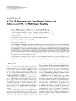
Figure 2: Normalized Gaussian window for different values of p.
Based on the above equation, the new S-transform can be
represented as
S
p
x
(t, f )
=
|
f |
p
√

2π

+∞
−∞
x(τ)exp

−
(t − τ)
2
f
2p
2

exp (−j2πfτ)dτ.
(8)
The parameter p can control the width of the window.
By finding an appropriate value of p,animprovedtime-
frequency concentration can be obtained. The window func-
tions with three different values of p are plotted in Figure 2,
where p
= 1 corresponds to the standard S-transform win-
dow. For p<1, the window becomes wider in the time do-
main, and for p>1, the window narrows in the time do-
main. Therefore, by considering the example from Section 2,
for the single sinusoid, a small value of p would provide
almost perfect concentration of the signal, whereas for the
Diracfunction,aratherlargevalueofp would produce a
good concentration in the time-frequency domain. It is im-
portant to mention that in the case of 0 <f<1, the opposite
is true.

Theoptimalvalueofp will be found based on the con-
centration measure proposed in [17], which has some fa-
vorable performance in comparison to other concentration
measures reported in [18–20]. The measure is designed to
minimize the energy concentration for any time-frequency
representation based on the automatic determination of
some time-frequency distribution parameter. This measure
is defined as
CM(p)
=
1

+∞
−∞

+∞
−∞


S
p
x
(t, f )


dt df
,(9)
where CM stands for a concentration measure.
There are two ways to determine the optimal value of p.
One is to determine a global, constant value of p for the en-

tire signal. The other is to determine a time-varying p(t),
which depends on each time instant considered. The first ap-
proach is more suitable for signals with the constant or slowly
varying frequency components. In this case, one value of p
will suffice to give the best resolution for all components.
The time-varying parameter is more appropriate for signals
with fast varying frequency components. In these situations,
depending on the time duration of the signal components,
it would be beneficial to use lower value of p (somewhere
in the middle of the particular component’s interval), and
to use higher values of p for the beginning and the end of
the component’s interval, so the component is not smeared
in the time-frequency plane. It is important to mention that
both proposed schemes for determining the parameter p are
the special cases of the algorithm which would evaluate the
parameter on any arbitrary subinterval, rather than over the
entire duration of the signal.
3.2.1. Algorithm for determining the time-invariant p
The algorithm for determining the optimized time-invariant
value of p is defined through the following steps.
(1) For p selected from a set 0 <p
≤ 1, compute S-
transform of the signal S
p
x
(t, f ) using (8).
(2) For each p from the given set, normalize the energy of
the S-transform representation, so that all of the rep-
resentations have the equal energy
S

p
x
(t, f ) =
S
p
x
(t, f )


+∞
−∞

+∞
−∞


S
p
x
(t, f )


2
dt df
. (10)
(3) For each p from the given set, compute the concentra-
tion measure according to (9), that is,
CM(p)
=
1


+∞
−∞

+∞
−∞


S
p
x
(t, f )


dt df
. (11)
(4) Determine the optimal parameter p
opt
by
p
opt
= max
p

CM(p)

. (12)
(5) Select S
p
x

(t, f )withp
opt
to be the WWOST
S
p
x
(t, f ) = S
p
opt
x
(t, f ). (13)
As it can be seen, the proposed algorithm computes the
S-transform for each value of p and, based on the com-
puted representation, it determines the concentration mea-
sure, CM(p), as an inverse of L
1
norm of the normalized
S-transform for a given p. The maximum of the concentra-
tion measure corresponds to the optimal p which provides
the least smear of
S
p
x
(t, f ).
It is important to note that in the first step, the value of
p is limited to the range 0 <p
≤ 1. Any negative value of p
corresponds to an nth root of a frequency which would make
the window wider as frequency increases. Similarly, values
Ervin Sejdi

´
cetal. 5
greater than 1 provide a window which may be too narrow in
the time domain. Unless the signal being analyzed is a super-
position of Delta functions, the value of p should not exceed
unity. As a special case, it is important to point out that for
p
= 0, the WWOST is equivalent to STFT with a Gaussian
window with σ
2
= 1.
3.2.2. Algorithm for determining p(t)
The time-varying parameter p(t)isrequiredforsignalswith
components having greater or abrupt changes. The algo-
rithm for choosing the optimal p(t) can be summarized
through the following steps.
(1) For p selected from a set 0 <p(t)
≤ 1, compute S-
transform of the signal S
p
x
(t, f ) using (8).
(2) Calculate the energy, E
1
,forp = 1. For each p from the
set, normalize the energy of the S-transform represen-
tation to E
1
, so that all of the representations have the
equal energy, and the amplitude of the components is

not distorted,
S
p
x
(t, f ) =

E
1
S
p
x
(t, f )


+∞
−∞

+∞
−∞


S
p
x
(t, f )


2
dt df
. (14)

(3) For each p from the set and a time instant t,compute
CM(t, p)
=
1

+∞
−∞


S
p
x
(t, f )


df
. (15)
(4) Optimal value of p for the considered instant t maxi-
mizes concentration measure CM(t, p),
p
opt
(t) = arg max
p

CM(t, p)

. (16)
(5) Set the WWOST to be
S
p

x
(t, f ) = S
p
opt
(t)
x
(t, f ). (17)
The main difference between the two techniques lies in
step (3). For the time invariant case, a single value of p is
chosen, whereas in the time-varying case, an optimal value of
p(t)isafunctionoftime.AsitisdemonstratedinSection 4,
the time-dependent parameter is beneficial for signals with
the fast varying components.
3.2.3. Inverse of the WWOST
Similarly to the standard S-transform, the WWOST can be
used as both an analysis and a synthesis tool. The inversion
procedure for the WWOST resembles that of the standard
S-transform, but with one additional constraint. The spec-
trum of the signal obtained by averaging S
p
x
(t, f )overtime
must be normalized by W(0, f ), where W(α, f ) represents
the Fourier transform (from t to α) of the window function,
w(t, σ( f )). Hence, the inverse WWOST for a signal, x(t), is
defined as
x(t)
=

+∞

−∞

+∞
−∞
1
W(0, f )
S
p
x
(τ, f )exp(j2πft)dτ df. (18)
In the case of a time-invariant p, it can be shown that
W(0, f )
= 1. In a general case, the Fourier transform of the
proposed modified window can only be determined numer-
ically.
4. WWOST PERFORMANCE ANALYSIS
In this section, the performance of the proposed scheme is
examined using a set of synthetic test signals first. Further-
more, the analysis of signals from an engine is also given.
The first part includes two cases: (1) a simple case involving
three slowly varying frequencies and (2) more complicated
cases involving multiple time-varying components. The goal
is to examine the performance of WWOST in comparison
to the standard S-transform. The proposed algorithm is also
compared to other time-frequency representations, such as
the short-time Fourier transform (STFT) and adaptive STFT
(ASTFT), to highlight the improved performance of the S-
transform with the proposed window width optimization
technique. In particular, the proposed algorithm can be used
for some classes of the signals for which the standard S-

transform would not be suitable.
As for the synthetic signals, the sampling period used in
the simulations is T
s
= 1/256 seconds. Also, the set of p
values, used in the numerical analysis of both test and the
knock pressure signals, is given by p
={0.01n : n ∈ N and
1
≤ n ≤ 100}. The ASTFT is calculated according to the con-
centration measure given by (9). In the definition of the mea-
sure, a normalized STFT is used instead of the normalized
WWOST. The standard deviation of the Gaussian window,
σ
gw
, is used as the optimizing parameter, where the window
is defined as
w
STFT
(t) =
1
σ
gw
√
2π
exp

−
t
2

2σ
2
gw

. (19)
The optimization for synthetic signals is performed on the
setofvaluesdefinedby
σ
gw
={n/128 : n ∈ N,1≤ n ≤ 128} (20)
and both the time-invariant and time-varying values of σ
gw
are calculated.
4.1. Synthetic test signals
Example 1. The first test signal is shown in Figure 3(a).Ithas
the following analytical expression:
x
1
(t) = cos

132πt +14πt
2

+cos

10πt − 2πt
2

+cos


30πt +6πt
2

,
(21)
where the signal exists only on the interval 0
≤ t<1. The sig-
nal consists of three slowly varying frequency components.
It is analyzed using the STFT (Figure 3(b)), ASTFT with
time-invariant optimum value of σ
gw
(Figure 3(c)), stan-
dard S-transform (Figure 3(d)), and the proposed algorithm
(Figure 3(f)). A Gaussian window is also used in the analy-
sis by the STFT, with standard deviations equal to 0.05. The
6 EURASIP Journal on Advances in Signal Processing
−5
0
5
Amplitude
00.20.40.60.81
Time (s)
(a)
0
50
100
Frequency (Hz)
00.20.40.60.81
Time (s)
(b)

0
50
100
Frequency (Hz)
00.20.40.60.81
Time (s)
(c)
0
50
100
Frequency (Hz)
00.20.40.60.81
Time (s)
(d)
0
0.5
1
Amplitude of CM
00.20.40.60.81
Time (s)
(e)
0
50
100
Frequency (Hz)
00.20.40.60.81
Time (s)
(f)
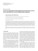
Figure 3: Test signal x
1

(t): (a) time-domain representation; (b) STFT of x
1
(t); (c) ASTFT of x
1
(t) with σ
opt
;(d)S
p
x
(t, f )ofx
1
(t) with p = 1
(standard S-transform); (e) concentration measure CM(p); (f) S
p
x
(t, f )ofx
1
(t) with the optimal value of p = .57.
optimum value of standard deviation for the ASTFT is calcu-
lated to be σ
opt
= 0.094. The colormap used for plotting the
time-frequency representations in Figure 3 and all the subse-
quent figures is a linear grayscale with values from 0 to 1.
The standard S-transform, shown in Figure 3(d), depicts
all three components clearly. However, only the first two
components have relatively good concentration, while the
third component is completely smeared in frequency. As
shown in Figure 3(b), the STFT provides better energy con-
centration than the standard S-transform. The ASTFT, de-

picted in Figure 3(c), shows a noticeable improvement for all
three components. The results with the proposed scheme is
shown in Figure 3(f) for p
= 0.57. The value of p is found ac-
cording to (12). For the determined value of p, the first two
components have higher concentration even than the ASTFT,
while the third component has approximately the same con-
centration.
In Figure 3(e), the normalized concentration measure is
depicted. The obtained results verify the theoretical predic-
tions from Section 3.2. For this class of signals, that is, the
signals with slowly varying frequencies, it is expected that
smaller values of p will produce the best energy concentra-
tion. In this example, the optimal value, found according to
(12), is determined numerically to be 0.57.
Based on the visual inspection of the time-frequency rep-
resentations shown in Figure 3, it can be concluded that the
proposed algorithm achieves higher concentration among
the considered representations. To confirm this fact, a per-
formance measure given by
Ξ
TF
=


+∞
−∞

+∞
−∞



TF(t, f )


dt df

−1
(22)
is used for measuring the concentration of the representa-
tion, where |TF(t, f )| is a normalized time-frequency repre-
sentation. The performance measure is actually the concen-
tration measure proposed in (9). A more concentrated rep-
resentation will produce a higher value of Ξ
TF
. Ta ble 1 sum-
marizes the performance measure for the STFT, the ASTFT,
the standard S-transform, and the WWOST.
Ervin Sejdi
´
cetal. 7
Table 1: Performance measure for the three time-frequency trans-
forms.
TFR Ξ
TF
STFT 0.0119
ASTFT 0.0131
Standard S-transform 0.0080
WWOST 0.0136
The value of the performance measure for the standard S-

transform is the lowest, followed by the STFT. The WWOST
produces the highest value of Ξ
TF
, and thus achieves a TFR
with the highest energy concentration amongst the trans-
forms considered.
Example 2. The signal in the second example contains mul-
tiple components with faster time-varying spectral contents.
The following signal is used:
x
2
(t) = cos

40π(t − 0.5) arctan (21t −10.5)
− 20π ln

(21t − 10.5)
2
+1

/21 + 120πt

+cos

40πt − 8πt
2

,
(23)
where x

2
(t) exists only on the interval 0 ≤ t<1. This
signal consists of two components. The first has a transi-
tion region from lower to higher frequencies, and the sec-
ond is a linear chirp. In the analysis, the time-frequency
transformations that employ a constant window exhibit a
conflicting issue between good concentration of the tran-
sition region for the first component versus good con-
centration for the rest of the signal. In order to numer-
ically demonstrate this problem, the signal is again ana-
lyzed using the STFT (Figure 4(a)), ASTFT with the opti-
mal time-invariant value of σ
gw
(Figure 4(c)), ASTFT with
the optimal time-varying value of σ
gw
(Figure 4(e)), stan-
dard S-transform (Figure 4(b)), the proposed algorithm
with both time-invariant (Figure 4(d)), and time-varying p
(Figure 4(f)). A Gaussian window is used for the STFT, with
σ
= 0.03. The optimum time-invariant value of the standard
deviation for the ASTFT is determined to be σ
opt
= 0.055.
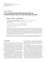
The standard deviation of the Gaussian window used
should be small in order for the STFT to provide relatively
good concentration in the transition region. However, as the
value of the standard deviation decreases, so is the concentra-
tion of the rest of the signal. To a certain extent, the standard

S-transform is capable of producing a good concentration
around the instantaneous frequencies at the lower frequen-
cies and also in the transition region for the first component.
However, at the high frequencies, the standard S-transform
exhibits poor concentration for the first component. The
WWOST with a time-invariant p enhances the concentra-
tion of the linear chirp, as shown in Figure 4(d). However the
concentration of the transition region of the first component
has deteriorated in comparison to the standard S-transform.
The concentration obtained with the WWOST with the time-
invariant p for this transition region is equivalent to the
poor concentration exhibited by the STFT. Even though the
ASTFT with both time-invariant and time-varying optimum
Table 2: Performance measures for the time-frequency representa-
tions considered in Example 2.
TFR Ξ
TF
STFT 0.0108
ASTFT with σ
opt
0.0115
ASTFT with σ
opt
(t) 0.0119
WWOST with p 0.0116
WWOST with p(t) 0.0124
values of standard deviation provide good concentration of
the linear FM component and the stationary parts of the sec-
ond component, the transition region of the second compo-
nent is smeared in time.

Figure 4(f) represents the signal optimized S-transform
obtained by using p(t). A significant improvement in the en-
ergy concentration is easily noticeable in comparison to the
standard S-transform. All components show improved en-
ergy concentration in comparison to the S-transform. Fur-
ther, a comparison of the representations obtained by the
proposed implementation of the S-transform and the STFT
shows that both components have higher energy concentra-
tion in the representation obtained by the WWOST with
p(t).
As mentioned previously, for this type of signals it is
more appropriate to use the time-varying p(t) rather than
a single constant p valueinordertoachievebetterconcen-
tration of the nonstationary data. By comparing Figures 4(d)
and 4(f), the component with the fast changing frequency
has better concentration with p(t) than a fixed p,whichis
calculated according to (12), while the linear chirp has simi-
lar concentration in both cases.
It would be beneficial to quantify the results by eval-
uating the performance measure again. The performance
measure is given by (22) and the results are summarized
in Tab le 2 . A higher value of the performance measure for
WWOST with p(t) reconfirms that the time-varying algo-
rithm should be used for the signals with fast changing com-
ponents. Also, it is worthwhile to examine the value of (22)
for the STFT and the ASTFT. The time-frequency represen-
tations of the signal obtained by the STFT and ASTFT al-
gorithms achieve smaller values of the performance measure
than WWOST. This supports the earlier conclusion that the
WWOST produces more concentrated energy representation

than the STFT and ASTFT. The WWOST with the time-
invariant value of p produces higher concentration than the
ASTFT with the optimum time-invariant value of σ
gw
,and
the WWOST with p(t) produces higher concentration than
the ASTFT with the optimum time-varying value of the
σ
gw
.
Example 3. Another important class of signals are those with
crossing components that have fast frequency variations. A
representative signal as shown in Figure 5(a) is given by
x
3
(t) = cos

20π ln (10t +1)

+cos

48πt +8πt
2

(24)
with x
3
(t) = 0 outside the interval 0 ≤ t<1. For this
class of signals, similar conflicting issues occur as in the
8 EURASIP Journal on Advances in Signal Processing

0
50
100
Frequency (Hz)
00.20.40.60.81
Time (s)
(a)
0
50
100
Frequency (Hz)
00.20.40.60.81
Time (s)
(b)
0
50
100
Frequency (Hz)
00.20.40.60.81
Time (s)
(c)
0
50
100
Frequency (Hz)
00.20.40.60.81
Time (s)
(d)
0
50

100
Frequency (Hz)
00.20.40.60.81
Time (s)
(e)
0
50
100
Frequency (Hz)
00.20.40.60.81
Time (s)
(f)
Figure 4: Comparison of different algorithms: (a) STFT of x
2
(t); (b) S
p
x
(t, f )ofx
2
(t) with p = 1 (standard S-transform); (c) ASTFT of x
2
(t)
with σ
opt
= 0.055; (d) S
p
x
(t, f )ofx
2
(t) with p = 0.73; (e) ASTFT of x

2
(t) with σ
opt
(t); (f) S
p
x
(t, f )ofx
2
(t) with the optimal p(t).
previous example; however, here exists an additional con-
straint, that is, the crossing components. The time-frequency
analysis is performed using the STFT (Figure 5(b)), the
ASTFT with the time-varying σ
gw
(Figure 5(c)), the standard
S-transform (Figure 5(d)), and the proposed algorithm for
the S-transform (Figure 5(f)). In the STFT, a Gaussian win-
dow with a standard deviation of 0.02 is used. Due to the
time-varying nature of the frequency components present in
the signal, the time-varying algorithm is used in the calcula-
tion of the WWOST in order to determine the optimal value
of p.
The representation obtained by the STFT depicts good
concentration of the higher frequencies, while having rela-
tively poor concentration at the lower frequencies. An im-
provement in the concentration of the lower frequencies
is obtained with the ASTFT algorithm. The standard S-
transform is capable of providing better concentration for
the high frequencies, but for the linear chirp, the concentra-
tion is equivalent to that of the STFT.

From the time-frequency representation obtained by the
WWOST, it is clear that the concentration is preserved at
high frequencies, while the linear chirp has significantly
higher concentration in comparison to the other represen-
tations. It is also interesting to note how p(t)variesbetween
0.6 and 1.0 as a function of time shown in Figure 5(e).Inpar-
ticular, p(t) is close to 1 at the beginning of the signal in order
to achieve good concentration of the high-frequency compo-
nent. As time progresses, the value of p(t)decreasesinorder
to provide a good concentration at the lower frequencies. To-
wards the end of the signal, p(t) increases again to achieve a
good time localization of the signal.
In Section 3, it has been stated that for the components
with faster variations, it is recommended that the time-
varying algorithm with the WWOST be used. In order to
substantiate that statement, the performance measure imple-
mented in the previous examples is used again and the results
are shown in Ta ble 3. The optimized time-invariant value of
the parameter p
opt
for this signal, found according to (12), is
determined numerically to be 0.71. These performance mea-
sures verify that the time-varying algorithm should be used
for the faster varying components. For comparison purposes,
the performance measures for the representations given by
Ervin Sejdi
´
cetal. 9
−2
0

2
Amplitude
00.20.40.60.81
Time (s)
(a)
0
50
100
Frequency (Hz)
00.20.40.60.81
Time (s)
(b)
0
50
100
Frequency (Hz)
00.20.40.60.81
Time (s)
(c)
0
50
100
Frequency (Hz)
00.20.40.60.81
Time (s)
(d)
0
0.5
1
Amplitude

00.20.40.60.81
Time (s)
(e)
0
50
100
Frequency (Hz)
00.20.40.60.81
Time (s)
(f)
Figure 5: Time-frequency analysis of signal with fast variations in frequency: (a) time-domain representation; (b) STFT of x
3
(t); (c) ASTFT
of x
3
(t) with σ
opt
(t); (d) S
p
x
(t, f )ofx
3
(t) with p = 1 (standard S-transform); (e) p(t); (f) S
p
x
(t, f )ofx
3
(t) with the optimal p(t).
Table 3: Performance measures for the time-frequency representa-
tions considered in Example 3.

TFR Ξ
TF
(noise-free) Ξ
TF
(SNR = 25 dB)
STFT 0.0106 0.0100
ASTFT with σ
opt
0.0121 0.0114
ASTFT with σ
opt
(t) 0.0122 0.0113
WWOST with p 0.0122 0.0110
WWOST with p(t) 0.0126 0.0116
the STFT and its time-invariant (σ
opt
= 0.048) and time-
varying adaptive algorithms are calculated as well. By com-
paring the values of the performance measure for different
time-frequency transforms, these values confirm the earlier
statement which assures that each algorithm for the WWOST
produces more concentrated time-frequency representation
in its respective class than the ASTFT.
In the analysis performed so far, it was assumed that the
signal-to-noise ratio (SNR) is infinity, that is, the noise-free
signals were considered. It would be beneficial to compare
the performance of the considered algorithms in the pres-
ence of additive white Gaussian noise in order to understand
whether the proposed algorithm is capable of providing the
enhanced performance in noisy environment. Hence, the sig-

nal x
3
(t) is contaminated with the additive white Gaussian
noise and it is assumed that SNR
= 25 dB. The results of such
an analysis are summarized in Tabl e 3. Even though, the per-
formance has degraded in comparison to the noiseless case,
the WWOST with p(t) still outperforms the other considered
representations.
4.2. Demonstration example
In order to illustrate the effectiveness of the proposed
scheme, the method has been applied to the analysis of en-
gine knocks. A knock is an undesired spontaneous autoigni-
tion of the unburned air-gas mixture causing a rapid in-
crease in pressure and temperature. This can lead to seri-
ous problems in spark-ignition car engines, for example,
10 EURASIP Journal on Advances in Signal Processing
−1
0
1
Amplitude (kPa)
0246
Time (ms)
(a)
0
1
2
3
Frequency (kHz)
0246

Time (ms)
(b)
0
1
2
3
Frequency (kHz)
0246
Time (ms)
(c)
0
1
2
3
Frequency (kHz)
0246
Time (ms)
(d)
0
1
2
3
Frequency (kHz)
0246
Time (ms)
(e)
0
1
2
3

Frequency (kHz)
0246
Time (ms)
(f)
Figure 6: Time-frequency analysis of engine knock pressure signal (17th trial): (a) time-domain representation; (b) STFT; (c) ASTFT with
σ
opt
(t); (d) S
p
x
(t, f ) with p = 1 (standard S-transform); (e) S
p
x
(t, f ) with p = 0.86; (f) S
p
x
(t, f ) with the optimal p(t).
environment pollution, mechanical damages, and reduced
energy efficiency [21, 22]. In this paper, a focus will be on
the analysis of knock pressure signals.
It has been previously shown that high-pass filtered pres-
sure signals in the presence of knocks can be modeled as
multicomponent FM signals [22]. Therefore, the goal of this
analysis is to illustrate how effectively the proposed WWOST
can decouple these components in time-frequency represen-
tation. A knock pressure signal recorded from a 1.81 Volk-
swagen Passat engine at 1200 rpm is considered. Note that the
signal is high-pass filtered with a cutoff frequency of 3000 Hz.
The sampling rate is f
s

= 100 kHz and the signal contains 744
samples.
The performance of the proposed scheme in this case is
evaluated by comparing it with that of the STFT, the ASTFT,
and the standard S-transform. The results are shown in Fig-
ures 6 and 7. These results represent two sample cases from
fifty trials. For the STFT, a Gaussian window, with a standard
deviation of 0.3 milliseconds, is used for both cases. The op-
timization of the standard deviation for the ASTFT is per-
formed on the set of values defined by σ
gw
={0.01n : n ∈
N
and 1 ≤ n ≤ 744} milliseconds.
A comparison of these representations show that the
WWOST performs significantly better than the standard S-
transform. The presence of several signal components can be
easily identified with the WWOST, but rather difficult with
the standard S-transform. In addition, both proposed algo-
rithms produce higher concentration than the STFT and the
corresponding class of the ASTFT. This is accurately depicted
through the results presented in Tab le 4 . The best concen-
tration is achieved with the time-varying algorithm, while
the time invariant value p produces slightly higher concen-
tration than the ASTFT with the time-invariant value of
σ
gw
(σ
opt
= 0.2 milliseconds for the signal in Figure 6 and

σ
opt
= 0.19 milliseconds for the signal in Figure 7).
The direct implication of the results is that the WWOST
could potentially be used for the knock pressure signal anal-
ysis. A major advantage of such an approach in compari-
son to some existing methods is that the signals could be
modeled based on a single observation, instead of multiple
Ervin Sejdi
´
cetal. 11
−1
0
1
Amplitude (kPa)
0246
Time (ms)
(a)
0
1
2
3
Frequency (kHz)
0246
Time (ms)
(b)
0
1
2
3

Frequency (kHz)
0246
Time (ms)
(c)
0
1
2
3
Frequency (kHz)
0246
Time (ms)
(d)
0
1
2
3
Frequency (kHz)
0246
Time (ms)
(e)
0
1
2
3
Frequency (kHz)
0246
Time (ms)
(f)
Figure 7: Time-frequency analysis of engine knock pressure signal (48th trial): (a) time-domain representation; (b) STFT; (c) ASTFT with
σ

opt
(t); (d) S
p
x
(t, f ) with p = 1 (standard S-transform); (e) S
p
x
(t, f ) with p = 0.87; (f) S
p
x
(t, f ) with the optimal p(t).
Table 4: Concentration measures for the two sample trials.
Trial Ξ
STFT
Ξ
ASTFTσ
opt
Ξ
ASTFTσ
opt
(t)
Ξ
p=1
Ξ
p
opt
Ξ
p
opt
(t)

17th trial 0.0057 0.0059 0.0068 0.0054 0.0065 0.0074
48th trial 0.0052 0.0054 0.0060 0.0053 0.0058 0.0069
realizations required by some other time-frequency methods
such as Wigner-Ville distribution [23], since the WWOST
does not suffer from the cross-terms present in bilinear trans-
forms.
4.3. Remarks
It should be noted that, in some cases, when implementing
the proposed algorithm, it may be beneficial to window the
signal before evaluating S
p
x
(t, f ) in step (1). This additional
step diminishes the effects of a discrete implementation. As
shown in [24], wideband signals might lead to some irregular
results unless they are properly windowed.
The STFT and the ASTFT are valuable signal decom-
position-based representations, which can achieve good en-
ergy concentration for a wide variety of signals. However,
throughout this paper, it is shown that the proposed opti-
mization of the window width used in the S-transform is
beneficial, and in presented cases, it outperforms other stan-
dard linear techniques, such as the STFT and the ASTFT.
It is also crucial to mention that the WWOST is designed
to achieve better concentration in the class of the time-
frequency representations based on the signal decomposi-
tion.
In comparison to the standard S-transform or the STFT,
the WWOST does have a higher computational complexity.
The algorithm for the WWOST is based on an optimiza-

tion procedure and requires a parameter tuning. However,
when compared to the transforms of similar group algo-
rithms (e.g., ASTFT), the WWOST has almost the same de-
gree of complexity.
The sampled data version of the standard S-transform
and their MATLAB implementations have been discussed in
12 EURASIP Journal on Advances in Signal Processing
several publications [5, 7, 25–27]. The WWOST is a straight-
forward extension of the standard S-transform. Therefore,
the sampled data version of the WWOST also follows the
steps presented in earlier publications.
5. CONCLUSION
In this paper, a scheme for improvement of the energy
concentration of the S-transform has been developed. The
scheme is based on the optimization of the width of the win-
dow used in the transform. The optimization is carried out
by means of a newly introduced parameter. Therefore, the
developed technique is referred to as a window width opti-
mized S-transform (WWOST). Two algorithms for parame-
ter optimization have been developed: one for finding an op-
timal constant value of the parameter p for the entire signal;
while the other is to find a time-varying parameter. The pro-
posed scheme is evaluated and compared with the standard
S-transform by using a set of synthetic test signals. The re-
sults have shown that the WWOST can achieve better energy
concentration in comparison with the standard S-transform.
As demonstrated, the WWOST is capable of achieving higher
concentration than other standard linear methods, such as
the STFT and its adaptive form. Furthermore, the proposed
technique has also been applied to engine knock pressure sig-

nal analysis, and the results have indicated that the proposed
technique provides a consistent improvement over the stan-
dard S-transform.
ACKNOWLEDGMENTS
Ervin Sejdi
´
c and Jin Jiang would like to thank the Natural Sci-
ences and Engineering Research Council of Canada (NSERC)
for financially supporting this work.
REFERENCES
[1] L. Cohen, Time-Frequency Analysis, Prentice Hall PTR, Engle-
wood Cliffs, NJ, USA, 1995.
[2]S.G.Mallat,A Wavelet Tour of Signal Processing,Academic
Press, San Diego, Calif, USA, 2nd edition, 1999.
[3] K. Gr
¨
ochenig, Foundations of Time-Frequency Analysis,
Birkh
¨
auser, Boston, Mass, USA, 2001.
[4] I. Djurovi
´
c and LJ. Stankovi
´
c, “A virtual instrument for time-
frequency analysis,” IEEE Transactions on Instrumentation and
Measurement, vol. 48, no. 6, pp. 1086–1092, 1999.
[5] R. G. Stockwell, L. Mansinha, and R. P. Lowe, “Localization of
the complex spectrum: the S-transform,” IEEE Transactions on
Signal Processing, vol. 44, no. 4, pp. 998–1001, 1996.

[6] S. Theophanis and J. Queen, “Color display of the localized
spectrum,” Geophysics, vol. 65, no. 4, pp. 1330–1340, 2000.
[7] C. R. Pinnegar and L. Mansinha, “The S-transform with win-
dows of arbitrary and varying shape,” Geophysics, vol. 68, no. 1,
pp. 381–385, 2003.
[8] C. R. Pinnegar and L. Mansinha, “The bi-Gaussian S-
transform,” SIAM Journal of Scientific Computing, vol. 24,
no. 5, pp. 1678–1692, 2003.
[9] M. Varanini, G. De Paolis, M. Emdin, et al., “Spectral analy-
sis of cardiovascular time series by the S-transform,” in Com-
puters in Cardiology, pp. 383–386, Lund, Sweden, September
1997.
[10] G. Livanos, N. Ranganathan, and J. Jiang, “Heart sound anal-
ysis using the S-transform,” in Computers in Cardiology,pp.
587–590, Cambridge, Mass, USA, September 2000.
[11] E. Sejdi
´
c and J. Jiang, “Comparative study of three time-
frequency representations with applications to a novel correla-
tion method,” in Proceedings of the IEEE International Confer-
ence on Acoustics, Speech and Signal Processing (ICASSP ’04),
vol. 2, pp. 633–636, Montreal, Quebec, Canada, May 2004.
[12] P.D.McFadden,J.G.Cook,andL.M.Forster,“Decomposi-
tion of gear vibration signals by the generalized S-transform,”
Mechanical Systems and Signal Processing, vol. 13, no. 5, pp.
691–707, 1999.
[13] A.G.Rehorn,E.Sejdi
´
c, and J. Jiang, “Fault diagnosis in ma-
chine tools using selective regional correlation,” Mechanical

Systems and Signal Processing, vol. 20, no. 5, pp. 1221–1238,
2006.
[14] P. K. Dash, B. K. Panigrahi, and G. Panda, “Power quality anal-
ysis using S-transform,” IEEE Transactions on Power Delivery,
vol. 18, no. 2, pp. 406–411, 2003.
[15] E. Sejdi
´
c and J. Jiang, “Selective regional correlation for pat-
tern recognition,” IEEE Transactions on Systems, Man, and Cy-
bernetics, Part A, vol. 37, no. 1, pp. 82–93, 2007.
[16] LJ. Stankovi
´
c, “Analysis of some time-frequency and time-
scale distributions,” Annales des Telecommunications, vol. 49,
no. 9-10, pp. 505–517, 1994.
[17] LJ. Stankovi
´
c, “Measure of some time-frequency distributions
concentration,” Signal Processing, vol. 81, no. 3, pp. 621–631,
2001.
[18] D. L. Jones and T. W. Parks, “A high resolution data-adaptive
time-frequency representation,” IEEE Transactions on Acous-
tics, Speech, and Signal Processing, vol. 38, no. 12, pp. 2127–
2135, 1990.
[19] T H. Sang and W. J. Williams, “R
´
enyi information and signal-
dependent optimal kernel design,” in Proceedings of the 20th
IEEE International Conference on Acoustics, Speech and Signal
Processing (ICASSP ’95), vol. 2, pp. 997–1000, Detroit, Mich,

USA, May 1995.
[20] W. J. Williams, M. L. Brown, and A. O. Hero III, “Uncertainty,
information, and time-frequency distributions,” in Advanced
Signal Processing Algorithms, Architectures, and Implementa-
tions II, vol. 1566 of Proceedings of SPIE, pp. 144–156, San
Diego, Calif, USA, July 1991.
[21]M.UrlaubandJ.F.B
¨
ohme, “Evaluation of knock begin in
spark-ignition engines by least-squares,” in Proceedings of the
IEEE International Conference on Acoustics, Speech and Signal
Processing (ICASSP ’05), vol. 5, pp. 681–684, Philadelphia, Pa,
USA, March 2005.
[22] I. Djurovi
´
c, M. Urlaub, LJ. Stankovi
´
c,andJ.F.B
¨
ohme, “Es-
timation of multicomponent signals by using time-frequency
representations with application to knock signal analysis,” in
Proceediongs of the European Signal Processing Conference (EU-
SIPCO ’04), pp. 1785–1788, Vienna, Austria, September 2004.
[23] D. K
¨
onigandJ.F.B
¨
ohme, “Application of cyclostationary and
time-frequency signal analysis to car engine diagnosis,” in Pro-

ceedings of IEEE International Conference on Acoustics, Speech,
and Signal Processing (ICASSP ’94), vol. 4, pp. 149–152, Ade-
laide, SA, Australia, April 1994.
[24] F. Gini and G. B. Giannakis, “Hybrid FM-polynomial phase
signal modeling: parameter estimation and Cram
´
er-Rao
bounds,” IEEE Transactions on Signal Processing, vol. 47, no. 2,
pp. 363–377, 1999.
Ervin Sejdi
´
cetal. 13
[25] R. G. Stockwell, S-transform analysis of gravity wave act ivity
from a small scale network of airglow imagers, Ph.D. disserta-
tion, The University of Western Ontario, London, Ontario,
Canada, 1999.
[26] C. R. Pinnegar and L. Mansinha, “Time-local Fourier analysis
with a scalable, phase-modulated analyzing function: the S-
transform with a complex window,” Signal Processing, vol. 84,
no. 7, pp. 1167–1176, 2004.
[27] C. R. Pinnegar, “Time-frequency and time-time filtering with
the S-transform and TT-transform,” DigitalSignalProcessing,
vol. 15, no. 6, pp. 604–620, 2005.