Báo cáo hóa học: " Research Article Maximum Likelihood DOA Estimation of Multiple Wideband Sources in the Presence of Nonuniform Sensor Noise" pdf

Hindawi Publishing Corporation
EURASIP Journal on Advances in Signal Processing
Volume 2008, Article ID 835079, 12 pages
doi:10.1155/2008/835079
Research Article
Maximum Likelihood DOA Estimation of Multiple Wideband
Sources in the Presence of Nonuniform Sensor Noise
C. E. Chen, F. Lorenzelli, R. E. Hudson, and K. Yao
Los Angeles EE Department, University of California, Los Angeles, CA 90095, USA
Correspondence should be addressed to C. E. Chen,
Received 1 March 2007; Revised 21 July 2007; Accepted 8 October 2007
Recommended by Sinan Gezici
We investigate the maximum likelihood (ML) direction-of-arrival (DOA) estimation of multiple wideband sources in the presence
of unknown nonuniform sensor noise. New closed-form expression for the direction estimation Cram
´
er-Rao-Bound (CRB) has
been derived. The performance of the conventional wideband uniform ML estimator under nonuniform noise has been stud-
ied. In order to mitigate the performance degradation caused by the nonuniformity of the noise, a new deterministic wide-
band nonuniform ML DOA estimator is derived and two associated processing algorithms are proposed. The first algorithm is
based on an iterative procedure which stepwise concentrates the log-likelihood function with respect to the DOAs and the noise
nuisance parameters, while the second is a noniterative algorithm that maximizes the derived approximately concentrated log-
likelihood function. The performance of the proposed algorithms is tested through extensive computer simulations. Simulation
results show the stepwise-concentrated ML algorithm (SC-ML) requires only a few iterations to converge and both the SC-ML and
the approximately-concentrated ML algorithm (AC-ML) attain a solution close to the derived CRB at high signal-to-noise ratio.
Copyright © 2008 C. E. Chen et al. This is an open access article distributed under the Creative Commons Attribution License,
which permits unrestricted use, distribution, and reproduction in any medium, provided the original work is properly cited.
1. INTRODUCTION
Direction-of-arrival (DOA) estimation has been one of the
central problems in radar, sonar, navigation, geophysics, and
acoustic tracking. A wide variety of high-resolution narrow-
band DOA estimators have been proposed and analyzed in

the past few decades [1–4]. The maximum likelihood (ML)
estimator, which shows excellent asymptotic performance,
plays an important role among these techniques. Many of the
proposed ML estimators are derived from the uniform white
noise assumption [4–6], in which the noise process of each
sensor is assumed to be spatially uncorrelated white Gaus-
sian with identical unknown variance. It is shown that under
this assumption the ML estimates of the nuisance parameters
(source waveforms/spectra and noise variance) can be ex-
pressed as a function of DOAs [7–9], and therefore the num-
ber of independent parameters to be estimated is reduced.
This procedure is called concentration, which substantially
reduces the search space and usually leads to a more efficient
implementation.
Recently, there has been a great interest in estimating the
DOAs for wideband sources, whose energy is spread over a
broad bandwidth. For example, acoustic signals can range
from 20 Hz to 20 kHz depending on the type of sources. For
wideband signals, many of the narrowband DOA estimation
algorithms cannot be directly applied since the phase differ-
ence between sensor pairs depends on not only the DOAs
but also the temporal frequencies. An intuitive way of gen-
eralizing a narrowband algorithm to wideband algorithm is
to use the discrete Fourier transform (DFT) to decompose
the signal into narrowband signals of different frequencies,
apply the narrowband algorithms to each component, and
fuse the overall estimation results. Better estimation accu-
racy is usually obtained when applying wideband algorithms
to wideband sources since the processing gain from the fre-
quency diversity is exploited. Various wideband ML estima-

tors have been proposed in the literature [10–12], most of
them are either derived under the uniform white noise as-
sumption [10, 12] or assume the noise spectrum is known or
estimated a priori [11].
The uniform white noise assumption is unrealistic in
many applications. For densely placed sensors, the noise can
be correlated and therefore should be modeled as a colored
random process. In order to reduce the number of nuisance
2 EURASIP Journal on Advances in Signal Processing
noise parameters, various noise modeling techniques have
been proposed in the literature [13–15]. In [13] the noise
is assumed to be an autoregressive moving-average (ARMA)
process whose parameters need to be estimated from a pre-
liminary step, while in [14] the noise covariance matrix is
modeled as a sum of Hermitian matrices known up to a
multiplicative scalar. In [16], a “despoking” technique is pro-
posed based on the assumption that the noise field is invari-
ant under two measurements of the array covariance. Closely
related to the ML estimator, a wideband DOA estimator in
the presence of colored noise has been proposed using the
generalized-least-squares approach [17]. The main restric-
tion of this method is that the signal spectral density matrices
are assumed to be the same for all frequency bins, which does
not hold for many wideband signals.
In several practical applications, the sensors are sparsely
placed so that the sensor noise is spatially uncorrelated. How-
ever, the noise power of each sensor can still be different due
to the variation of the manufacturing process or the imper-
fection of array calibration. As a result, the noise covariance
matrix can be modeled as a diagonal matrix where the diag-

onal elements in general are not identical. It is crucial to note
that this modeling is not a special case of the ARMA model-
ing [13], as is explained in [18]. Furthermore, the DOA esti-
mators derived from either the uniform white noise assump-
tion or the general colored noise modeling techniques may
not give satisfactory results in this nonuniform uncorrelated
noise environment since the algorithm derived from the uni-
form white noise assumption blindly treats all sensors equally
and the general colored noise modeling technique neglects
the fact that the sensor noise is uncorrelated. Motivated by
the arguments above, a narrowband ML DOA estimator un-
der this nonuniform sensor noise model has been recently
derived [18]. Yet to the best of our knowledge, neither the
nonuniform wideband ML DOA estimator under the same
noise model nor its theoretical bound has ever been investi-
gated in the literature.
Inthispaper,wederiveanewwidebandMLDOAes-
timator and a new closed-form expression of the Cram
´
er-
Rao bound (CRB) in the presence of unknown nonuni-
form noise. Our expression can be viewed as an extension
of [12] to nonuniform noise scenarios and a generalization
of [18] to a wideband signal model. It turns out that the
derived nonuniform wideband ML DOA estimator cannot
be concentrated analytically, and therefore the direct imple-
mentation would require an exhaustive search in the joint-
parameter space. In order to reduce the complexity, two dif-
ferent algorithms have been proposed. The first algorithm is
based on an iterative procedure which stepwise concentrates

the log-likelihood function, while the second is a noniter-
ative algorithm that maximizes the derived approximately-
concentrated (AC) log-likelihood function.
The rest of the paper is organized as follows. The wide-
band signal model is introduced in Section 2, and the con-
ventional wideband uniform ML DOA estimator (uniform-
ML estimator) [12]isreviewedinSection 3.InSection 4, the
new wideband nonuniform ML estimator (nonuniform-ML
estimator) is first derived, and two new algorithms are pro-
posed. The derived CRB is also presented in the same section.
The performance of the proposed algorithms is studied and
compared with the CRB through computer simulations and
is shown in Section 5. The paper is concluded in Section 6.
Throughout this paper, the superscripts T,
∗, H,and†
stand for the transpose, conjugate, conjugate transpose, and
pseudoinverse of a matrix while
⊗ and  stand for the Kro-
necker and Hadamard matrix product operators. The real
part and imaginary part of a matrix are denoted by R
{·}
and I{·}, respectively, while the Euclidean norm is denoted
as
·, 1 is the vector of all ones and I is the identity matrix.
2. WIDEBAND SIGNAL MODEL
Let there be M wideband sources in the far-field of a P-
element arbitrarily distributed array (M<P). For simplicity,
we assume the sources and the array lie in the same plane,
and θ
m

denotes the DOA of the mth source with respect
to the centroid of the array, m
= 1, , M.Thenumberof
sources is assumed to be known or has been correctly es-
timated by [19]. Without loss of generality, we set the ar-
ray centroid to be at the origin, and the position vector of
each sensor is expressed as r
p
= [r
p
cos(φ
p
), r
p
sin(φ
p
)]
T
,
p
= 1, , P. For a uniform circular array (UCA), r
p
can be
further simplified to r
p
= [R cos(2π(p − 1)/P), R sin(2π(p −
1)/P)]
T
,whereR is the radius of the UCA. In this paper, we
derive our wideband algorithms and the CRB for arrays of

arbitrary geometry, while the simulation is performed under
a UCA setting (Section 5).
For a general array geometry, the time-delay (in samples)
from the mth source to the pth sensor relative to the centroid
can be expressed as t
(m)
p
= r
p
F
s
cos(θ
m
−φ
p
)/v,whereF
s
is the
sampling frequency and v is the known propagation speed
of wave. The received waveform by the pth sensor at time
instant n can then be expressed as
x
p
(n) =
M

m=1
s
(m)


n − t
(m)
p

+ w
p
(n), (1)
for n
= 0, , N − 1. Here N denotes the number of samples
per frame, s
(m)
(n) is the signal waveform of the mth source,
and w
p
(n) is the sensor noise at the pth sensor. We transform
(1) into the frequency domain via the DFT, which allows the
signal model to be expressed with multiplicative steering vec-
tors instead of time delays.
After applying the N-point DFT to (1), we obtain the fol-
lowing signal model:
X(k)
= D(k)S(k)+W(k), (2)
where k
= 0, , N − 1. Here X(k) = [X
1
(k), , X
P
(k)]
T
de-

notes the spectrum of the observed waveform, and S(k)
=
[S
(1)
(k), , S
(m)
(k)]
T
and W(k) = [W
1
(k), , W
P
(k)]
T
are the complex source and noise spectrum, respectively.
D(k)
= [d
(1)
(k), , d
(M)
(k)] is called the steering matrix,
where d
(m)
(k) = [d
(m)
1
(k), , d
(m)
p
(k)]

T
is the steering vec-
tor of the mth source. Let the sensor response from the
mth source to the pth sensor be a
p
(k,θ
m
), then d
(m)
p
(k) =
a
p
(k,θ
m
)e
− j2πkt
(m)
p
/N
.
C. E. Chen et al. 3
Throughout this paper, we assume the source spectrum
S(k) to be deterministic and unknown while the noise spec-
trum W(k) is modeled as a spatially uncorrelated zero-mean
white Gaussian process with the following covariance matrix:
Q
= E

W(k)W(k)

H

=
⎡
⎢
⎢
⎢
⎢
⎣
q
1
0
q
2
.
.
.
0 q
p
⎤
⎥
⎥
⎥
⎥
⎦
.
(3)
3. REVIEW ON THE WIDEBAND
MAXIMUM-LIKELIHOOD DOA ESTIMATOR IN
THE PRESENCE OF UNIFORM SENSOR NOISE

In this section, we review on the conventional uniform noise
wideband ML DOA estimator (uniform-ML estimator) [12].
The estimator is derived from the wideband deterministic
signal model (2) along with the uniform white noise assump-
tion of Q
= σ
2
I.
Denote Ω
= [Θ
T
, S
T
, σ
2
]
T
as the vector of all the un-
known parameters in the model, where
Θ
= [θ
1
, , θ
M
]
T
,
S
=


S(1)
T
, , S

N
2

T

T
,
(4)
then the likelihood function of Ω can be expressed as
f (Ω)
=
1
π
PN/2
σ
PN
exp

−
1
σ
2
N/2

k=1



g(k)


2

,(5)
where
g(k)
= X(k) − D(k)S(k). (6)
Take the logarithm of (5) and neglect all the constant terms,
the log-likelihood function L(Ω) can be expressed as
L(Ω)
=−
PN
2
log σ
2
−
1
σ
2
N/2

k=1


g(k)



2
. (7)
It follows that the maximum likelihood estimator for Ω is
simply

Ω = arg max
Ω
L(Ω). (8)
It is clear that the dependency of L(Ω)withrespectto
Θ and S is through
g(k)
2
, which is independent of σ
2
.It
follows that a concentrated ML estimator for Θ and S can be
obtained immediately by


Θ,

S

=
arg min
Θ,S
N/2

k=1



g(k)


2
. (9)
Here S(k)andΘ are referred to as the linear and nonlinear
parameters, respectively, since the noise corrupted data X(k)
is linear in S(k) but nonlinear in Θ.
A standard procedure of solving this type of joint maxi-
mization problem which contains both linear and nonlinear
parameters is as follows. (1) Fix the nonlinear parameter and
derive the optimal estimator of the linear parameter. (2) Sub-
stitute the linear parameter by its estimator in the original
objective function and obtain a concentrated objective func-
tion that contains only the nonlinear parameter. (3) Find the
estimate for the nonlinear parameter by optimizing the con-
centrated objective function. (4) Find the estimate for the lin-
ear parameter by substituting the estimate for the nonlinear
parameter back to its estimator. Follow this procedure, the
original joint optimization problem is reduced to a separable
optimization problem.
For our wideband DOA estimation problem (9), once Θ
is fixed, the estimator for S is simply the least-squares solu-
tion

S(k) = D(k)
†
X(k). (10)
Substituting


S(k)backto(9) and the estimator for Θ can
then be written as

Θ = arg min
Θ
N/2

k=1


X(k) − D(k)
†
X(k)


2
. (11)
Note that we start with a joint optimization problem (8)of
dimension M + PN + 1, and then reduce it analytically to a
much smaller optimization problem (11) of dimension M.
Many numerical optimization algorithms in the literature
can be used to solve

Θ [20–26]. No methods are guaranteed
to achieve the global optimum in general.
4. DERIVATION OF THE WIDEBAND
MAXIMUM-LIKELIHOOD DOA ESTIMATOR AND
THE CRB IN THE PRESENCE OF NONUNIFORM
SENSOR NOISE

In this section, we derive a new nonuniform wideband DOA
ML estimator and the CRB in the presence of nonuniform
sensor noise. Unlike the uniform white noise model used in
Section 3, the noise covariance matrix Q is now modeled as
a diagonal matrix with nonidentical diagonal elements (3).
Define Ψ
=

Θ
T
, S
T
, q
T

T
as the vector of all the un-
known parameters in the model, where q
= [q
1
, , q
P
]
T
is
the vector of the diagonal elements of Q, then the likelihood
function of Ψ can be expressed as
f (Ψ)
=
1


π
P
det Q

N/2
exp

−
N/2

k=1
g(k)
H
Q
−1
g(k)

. (12)
Taking the logarithm of (12) and neglecting all the constant
terms, we have the following log-likelihood function L(Ψ):
L(Ψ)
=−
N
2
P

p=1
log q
p

−
N/2

k=1
g(k)
2
, (13)
where
g(k) = Q
−1/2
g(k) =

X(k) −

D(k)S(k),

X(k) = Q
−1/2
X(k),

D(k) = Q
−1/2
D(k).
(14)
4 EURASIP Journal on Advances in Signal Processing
g(k),

X(k), and

D(k) can be viewed as the “spatially whit-

ened” version of g(k), X(k), and D(k), respectively.
It follows that the maximum likelihood estimator for Ψ
is simply

Ψ = arg max
Ψ
L(Ψ), (15)
which is a joint optimization problem of dimension M +
MN + P. Since the estimation of Θ is our only interest, we
would like to reduce the search space analytically as is done
in the derivation of the uniform-ML estimator.
Unlike the uniform noise case, now the estimation of
Θ and S is through
g(k)
2
, which is also a function of q.
Therefore, the estimation of signal parameters and noise pa-
rameters are interrelated. We approach this problem by first
fixing Θ and S in (15) and deriving an estimator of q as a
function of Θ and S. After taking the gradient of L(Ψ)with
respect to q and setting it to zero, the following estimator for
q
p
is obtained:
q
p
=
2
N
N/2


k=1




g(k)

p



2
(16)
=
2
N


g
p


2
,
(17)
where [g(k)]
p
denotes the pth element of the residual vector,
g(k), and

g
p
=


g(1)

p
, ,

g

N
2

p

T
. (18)
Let
q = [q
1
, , q
P
]
T
and substitute q by q in (13), we
have the following concentrated log-likelihood function of
Θ and S :
L(Θ, S)

=−
N
2
P

p=1
log q
p
−
N/2

k=1
P

p=1



g(k)

p


2
q
p
=
N
2


P

log

N
2

−
1

−
P

p=1
log


g
p


2

.
(19)
It follows that a concentrated ML estimator for Θ and S can
be expressed as


Θ,


S

= arg max
Θ,S
−
P

p=1
log


g
p


2
. (20)
To co n c e n t r a t e L(Θ, S) further, one would fix Θ and derive an
estimator for S that maximizes L(Θ, S). Unfortunately, a sep-
arable closed-form estimator for S that maximizes (20)seems
to be analytically unavailable, and this prevents us from fur-
ther simplifications.
On the other hand, we can approach the problem by fix-
ing Θ and q in (15)andderiveanestimatorforS. The result-
ing estimator

S is again the least-square solution

S(k) =


D(k)
†

X(k). (21)
Substituting S(k)by

S(k) into (13), the concentrated log-
likelihood function of Θ and Q is obtained as
L(Θ, Q)
=−
N
2
P

p=1
log q
p
−
N/2

k=1


P
⊥

D(k)

X(k)



2
, (22)
where
P
⊥

D(k)
= I −

D(k)

D(k)
†
. (23)
As a result, a concentrated ML estimator for Θ and Q is
obtained as
(

Θ,

Q) = arg max
Θ,Q
L(Θ, Q). (24)
Again, no closed-form estimator of Q which maximizes
(22)withfixedΘ seems to be available, and therefore no fur-
ther concentration can be performed. Instead of direct im-
plementing (15), (20), or (24), which requires an exhaustive
search in the joint parameter space, we propose the following

two novel algorithms to reduce the complexity.
4.1. Stepwise-concentrated maximum likelihood
algorithm (SC-ML)
The first proposed algorithm is based on the technique of
stepwise concentration (SC), which is conceptually related to
the alternating projection (AP) [2], iterative quadratic maxi-
mum likelihood (IQML) [27], and method of direction esti-
mation (MODE) [28]. The idea of this technique is to step-
wise concentrate the log-likelihood function in an iterative
manner, which has been successfully applied in [18]. In this
subsection, we use the same concept to numerically concen-
trate (20).
Insert (21) into (20), we have the following alternative
expression:


Θ,

Q

=
arg max
Θ,Q
L(Θ, Q), (25)
where
L(Θ, Q) =−
P

p=1
log



g
p


2
,
(26)
g
p
=

g(1)

p
, ,

g

N
2

p

T
,
(27)
g(k) = X(k) − D(k)


D(k)
†

X(k).
(28)
Using (17), (21), and (25), we have the iterative proce-
dure shown in Algorithm 1.
In the proposed SC-ML, we initialize the procedure by
assuming the noise covariance matrix

Q = I. In fact, this ini-
tialization is less restrictive than it appears. For a more gen-
eral noise covariance matrix

Q = αI,whereα is an arbitrary
positive constant, it is easy to show that for a fixed α, the first
term of (22) is simply a constant while the second term is
not a function of α. As a result, the DOA estimate obtained
at step 1 is independent of the value of α, which allows us to
C. E. Chen et al. 5
Initialization:Iter= 0. Set

Q = I (same as setting q = 1).
Loop start:
Step 1. Find the estimate of Θ as

Θ = arg max
Θ
L(Θ,


Q), where L(Θ, Q)isdefinedasin(26)–(28). Iter = Iter + 1.
Step 2. Use the obtained

Θ and q to compute

S(k) through (21).
Step 3. Use the obtained

Θ and

S(k) to compute a refined q through (17).
Loop end:
Repeat steps 1–3 a few times to obtain the final estimate.
Algorithm 1: Iterative procedure of the proposed SC-ML algorithm.
simply set α = 1(

Q = I) for a more general uniform noise
initialization. The convergence of the algorithm follows from
the fact that a new set of parameters is found in each iteration
such that
L(

Θ,

Q) is monotonically increasing. This ensures
that the algorithm converges to at least a local optimal point.
Simulation results (Section 5) also show that only two itera-
tions are required to obtain a solution close to the CRB.
It is also interesting to observe that the concentrated log-
likelihood function (26) used in the SC-ML in the uniform

case does not degenerate to the log-likelihood used in the
uniform-ML estimator (11). This is because when we sub-
stitute (17) into (13), the a priori information on the struc-
ture of the noise covariance matrix has been exploited ex-
plicitly. This prior information is processed through the log-
arithmic operation which serves as an “equalizer” assigning
lower weighting to noisier sensors.
Like the uniform-ML estimator, the major computa-
tional burden of the SC-ML is in the DOA estimation stage of
step 1, where a highly nonlinear optimization problem needs
to be solved. Many numerical algorithms designed for solv-
ing (11) in the literature can be easily modified to carry out
step 1.
4.2. Approximately concentrated maximum likelihood
algorithm (AC-ML)
In Section 4.1, an iterative maximum likelihood wideband
DOA estimation algorithm is presented. The algorithm step-
wise concentrates the DOAs and the nuisance parameters,
and it only requires a few iterations to converge to a solution
close to the CRB (see Section 5). In this subsection, we pro-
pose a new algorithm which is noniterative and has an MSE
performance comparable to the SC-ML.
Clearly, a naive noniterative algorithm is already avail-
able, which can be obtained by simply running the SC-ML
for just one single iteration without any refinement. There-
fore, for the proposed noniterative algorithm to be useful, it
must give a consistently better performance in comparison
to the 1st-iteration estimate of the SC-ML. In Section 4.1,we
describe the procedure of the SC-ML, which initializes the
algorithm by setting


Q = I. Intuitively, a better estimator can
be developed if the algorithm starts with a more informative

Q.
This is the main idea of our AC-ML. Instead of initializ-
ing the algorithm with a constant
q = 1,weseeka
ˇ
q(Θ)so
that as we optimize over Θ, we optimize over
ˇ
q simultane-
ously. For the AC-ML, we propose the following
ˇ
q:
ˇ
q
=

ˇ
q
1
, ,
ˇ
q
P

T
, (29)

where
ˇ
q
p
=
2
N







ˇ
g(1)

p
, ,

ˇ
g

N
2

p

T






2
,
(30)
ˇ
g(k)
= X(k) − D(k)D(k)
†
X(k).
(31)
The proposed
ˇ
q has the same expression as
q in (17), ex-
cept the S(k) is now approximated by D(k)
†
X(k). Recall
D(k)
†
X(k) is the ML estimator for S(k) under the white noise
assumption. At high SNR region, D(k)
†
X(k)appearstobea
good approximation for S(k)andasaconsequence
ˇ
q pro-
vides a nice estimate of the underlying nonuniform noise.

With this approximation, we now have the proposed AC-ML:

Θ = arg min
Θ
P

p=1
log



g
p


2
, (32)
where
g
p
=


g(1)

p
, ,


g


N
2

p

T
,
(33)
g(k) = X(k) − D(k)
ˇ
D(k)
†
ˇ
X(k),
(34)
ˇ
D(k)
=
ˇ
Q
−1/2
D(k),
ˇ
X(k)
=
ˇ
Q
−1/2
X(k),

ˇ
Q
= diag{
ˇ
q
}.
(35)
Strictly speaking, the AC-ML is a suboptimal algorithm
and can be made an iterative algorithm by the same stepwise-
concentration technique. However, it is shown in the simu-
lations of Section 5 that the AC-ML gives almost the same
performance of the SC-ML within the SNR regions of in-
terest and provides a solution close to the derived CRB high
SNR, which suggests no significant MSE performance can be
gained through iterative refinement.
The complexity of the AC-ML is again dominated by
the DOA estimation stage (32), where a global optimization
problem needs to be solved. To be more specific, the com-
plexity is dominated by the pseudoinverse operation in (31)
6 EURASIP Journal on Advances in Signal Processing
and (34), and the logarithmic function evaluation in (32).
For the SC-ML, one pseudoinverse operation in (28)andone
logarithmic function evaluation are required for every testing
Θ in each iteration. A more detailed complexity comparison
between the SC-ML and AC-ML depends on the choice of
optimization methods. Nonetheless, if we assume the same
optimization algorithm for both estimators and the efforts
of each iteration in the SC-ML are roughly the same, we can
conclude the complexity of the AC-ML is less than that of the
SC-ML running two iterations.

4.3. The Cram
´
er-Rao bound
The CRB is probably the most well-known theoretical bound
of the variances of unbiased estimators. In this subsection,
we present the results of the CRB derived from the wideband
signal and nonuniform sensor noise model (Section 2). The
newly derived nonuniform CRB can be viewed as an exten-
sion of [29] to a more general multiple sources/nonuniform
noise scenario and the wideband generalization of the nar-
rowband deterministic expression shown in [18]. The de-
tailed derivation is shown in Appendix A.
Lemma 1. TheinverseoftheCRBmatrixforΘ can be ex-
pressed as
CRB
−1
ΘΘ
= 2R

N/2

k=1


E(k)
H
P
⊥

D(k)


E(k)

 R
S
(k)
T


, (36)
where
P
⊥

D(k)
= I −

D(k)

D(k)
†
,

E(k) = Q
−1/2
E(k),
E(k)
=

d

dθ
1
d
(1)
(k), ,
d
dθ
M
d
(M)
(k)

,
R
S
(k) = S(k)S(k)
H
.
(37)
When the sensor noise is uniform, (36) degenerates to
CRB
−1
ΘΘ,uni
=
2
σ
2
R

N/2


k=1

E(k)
H
P
⊥
D(k)
E(k)

 R
S
(k)
T


.
(38)
From (36) we observe that CRB
−1
ΘΘ
contains contribu-
tions from all frequency bins through a direct summation.
The contribution from each frequency bin is an elementwise
matrix product of the geometry factor,

E(k)
H
P
⊥


D(k)

E(k), and
the spectral factor, R
S
(k)
T
. The geometry factor provides a
measure of geometric relations between the sources and the
sensor array, and the significance of each sensor is adjusted by
its variance through

D(k)and

E(k). Q
−1/2
acts as the mani-
fold transformation matrix which spatially prewhitens D(k)
and E(k) so that noisy sensors are given less weights. The
spectral factor R
S
(k)
T
, on the other hand, provides a mea-
sure of correlations among M sources. For those frequency
bins where no signals are present, the spectral factors are just
zero matrices and thus do not contribute to CRB
−1
ΘΘ

as is in-
tuitively expected.
Under the single source scenario, (36) can be further sim-
plified as
CRB
−1
= 2
N/2

k=1

e(k)
2


d(k)
2
−|

d(k)
H
e(k)|
2

|
S(k)|
2


d(k)

2
.
(39)
Here we have changed the notation S(k)toS(k), since S(k)
is just a complex scalar in the single source scenario. Gen-
eralizing the results of [18, 30] we can define the wideband
array-signal-to-noise ratio (ASNR):
ASNR
=
2
NP
N/2

k=1



d(k)


2
|S(k)|
2
, (40)
which is a measure of the averaged SNR. If we further assume
the sensors to be omnidirectional with unit sensor response
(a
p
(k,θ) = 1) and have the same noise variance σ
2

,(40)be-
comes
ASNR
=
2
Nσ
2
N/2

k=1


S(k)


2
,
(41)
which is the same as the common definition for the SNR.
This quantity (40) will be fixed when we investigate the effect
of the nonuniformity of noise in Section 5.
5. SIMULATIONS
In this section, we present the simulation results of the pro-
posed algorithms under varies of simulation examples. While
the assumed signal models and the proposed algorithms are
derived for general wideband applications, the simulation
examples demonstrated in this section will be performed un-
der the acoustic settings.
The simulation is performed under a setup of an 8-
element UCA with a radius R

= 0.25 meter. Each micro-
phone on the UCA is assumed to be omnidirectional with
unity sensor gain (a
p
(k,θ
m
) = 1) and perfectly synchro-
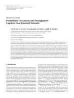
nized. Three human speech recordings sampled at 16 kHz
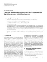
are used as our wideband sources (Figure 1), and a frame
of 1024 snapshots (64 milliseconds) has been extracted from
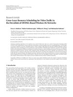
each recording (see Figures 2 and 3). The propagation speed
of acoustic wave is set to be 345 m/s and is assumed to be
known.
Throughout the simulation, the DOA estimation opera-
tions required in step 1 of the SC-ML and (32) of the AC-ML
are performed by the alternating maximization (AM) algo-
rithm [31], implemented by a coarse search of 1
◦
step size
followed by the golden section fine search. Theoretical results
as well as the relative capabilities of the proposed algorithms
(SC-ML and AC-ML) are shown in the following examples.
(1) The wideband CRB in the presence of
nonuniform sensor noise
Unlike most simulation settings presented in the literature,
we choose a UCA rather than a uniform linear array (ULA)
C. E. Chen et al. 7
−1
0
1

00.20.40.60.811.21.4
Time (s)
Amplitude
(a)
−1
0
1
00.20.40.60.811.21.4
Time (s)
Amplitude
(b)
−1
0
1
00.20.40.60.811.21.4
Time (s)
Amplitude
(c)
Figure 1: Acoustic waveforms of three human speech recordings.
−4
−2
0
2
4
Time index (n)
100 200 300 400 500 600 700 800 900 1000
|s
(1)
(n)|
(a)

−4
−2
0
2
4
Time index (n)
100 200 300 400 500 600 700 800 900 1000
|s
(2)
(n)|
(b)
−4
−2
0
2
4
Time index (n)
100 200 300 400 500 600 700 800 900 1000
|s
(3)
(n)|
(c)
Figure 2: Time domain acoustic waveforms of the extracted frame
(after normalization).
0
5
10
Frequency index (k)
50 100 150 200 250 300 350 400 450 500
|S

(1)
(k)|
(a)
0
5
10
Frequency index (k)
50 100 150 200 250 300 350 400 450 500
|S
(2)
(k)|
(b)
0
2
4
6
8
Frequency index (k)
50 100 150 200 250 300 350 400 450 500
|S
(3)
(k)|
(c)
Figure 3: Magnitude spectrum of the extracted frame (after nor-
malization).
as our array geometry. Although the ULA is easy to ana-
lyze and provides the largest array aperture when given the
same number of sensors, it has a few restrictions. First, the
ULA is unable to distinguish DOAs symmetric to the array
line and therefore is usually applied to applications where

the field of view (FOV) is within 180
◦
[32]. Second, the per-
formance of the ULA is nonuniform. For example, the DOA
estimation performance degrades considerably near the end-
fire of a ULA, while the UCA always gives uniform perfor-
mance over the whole FOV for single source DOA estimation
[29, 33]. As a result, the UCA has been considered as one
of the most favorable geometries used in DOA estimation.
However, this nice property holds only under the uniform
white noise assumption. When the sensor noise is nonuni-
form, the CRB becomes a function of the DOAs and the
dependency varies with the distribution of the noise vari-
ances.
In the first example, we investigate how the nonunifor-
mity of the noise affects the theoretical capabilities of the
DOA estimation. Source 1 is chosen as our wideband source
in this example and DOA1 is assumed to be 90
◦
relative to
the array. Let us define the worst-noise-power ratio (WNPR)
[18]:
WNPR
=
σ
2
max
σ
2
min

(42)
as a measurement of nonuniformity of sensor noise, where
σ
2
max
and σ
2
min
are the largest and smallest noise variance,
8 EURASIP Journal on Advances in Signal Processing
1.5
2
2.5
3
3.5
4
4.5
×10
−3
CRB
0 50 100 150 200 250 300 350
DOA (deg)
Realization 1
Realization 2
Realization 3
Realization 4
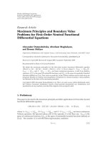
Figure 4: CRB versus the source DOA.
2
2.5
3

3.5
4
4.5
5
5.5
6
7
6.5
×10
−3
CRB
2 4 6 8 10 12 14 16 18 20
WNPR
MSE of uniform-ML
Mean of CRB
Figure 5: Comparison of the MSE of the uniform-ML estimator
with the CRB.
respectively. In each Monte Carlo run, we fix the WNPR
and randomly choose two sensor locations in the UCA, one
with noise variance σ
2
min
and the other σ
2
max
= WNPRσ
2
min
.
The noise variance of the rest of the sensors are assigned

according to a uniform distribution within the interval
(σ
2
min
, σ
2
max
).Inordertoreducetheeffect of SNR fluctua-
tions, the noise variance is scaled such that the ASNR defined
in (40)isfixedat20dB.
In Figure 4, we fix the WNPR to be 20 and perform the
simulation described as before. The CRBs from four random
realizations in the Monte Carlo runs have been plotted with
10
−4
10
−3
10
−2
10
−1
10
0
10
1
10
2
MSE
SNR1 (dB)
−10 −50 5 1015202530

Uniform-ML
AC-ML
CRB
SC-ML (iteration 1)
SC-ML (iteration 2)
Figure 6: Comparison of the DOA estimation MSEs and the CRB
(single source case).
respect to the DOA. It is clear that the CRB of a UCA in the
presence of nonuniform noise is no longer a constant over
the FOV and depends on the nonuniformity of noise. It is
also observed that the nonuniform CRB has a period of 180
◦
.
This is true for any nonisotropic planar array, which can be
easily verified from (39) (see Appendix B).
Figure 5 further quantifies the relation of the nonuni-
formity of the CRB with respect to the WNPR. The mean
and standard deviation (std) of the CRB shown on the error
bar of the figure is estimated by averaging over 10000 Monte
Carlo simulations. As expected, the CRB has a larger std as
the WNPR increases and therefore is more nonuniform. We
also plot the MSE of the uniform-ML estimator [12]under
the same simulation conditions. The vertical gap between the
MSE of the uniform-ML estimator and the mean of CRB
shows the average performance degradation if the nonuni-
formity of noise is ignored. A larger average performance
degradation is also observed at high WNPR. This justifies
the development of the SC-ML and AC-ML presented in this
work. When the noise is uniform (WNPR
= 1), the perfor-

mance loss between the uniform-ML estimator and the CRB
is zero.
(2) Single source wideband DOA estimation
In the second example, we investigate the performance of the
SC-ML and the AC-ML in estimating the DOA of a single
source in the presence of nonuniform sensor noise. The set-
ting of the simulation is the same as the previous example
except now the covariance of the sensor noise is fixed to
Q
= σ
2
diag{1, 20, 1.5, 1, 10,1,2, 5}. (43)
The MSEs and the CRB are plotted with respect to the SNR
of the 1st sensor for comparison.
C. E. Chen et al. 9
10
−4
10
−3
10
−2
10
−1
10
0
10
1
10
2
MSE

SNR1 (dB)
0 5 10 15 20 25 30
Uniform-ML
AC-ML
CRB
SC-ML (iteration 1)
SC-ML (iteration 2)
Figure 7: Comparison of the MSEs and the CRB in estimating
DOA1 (two sources case).
Figure 6 shows the MSE performance of the SC-ML, AC-
ML, and the conventional uniform-ML estimator with re-
spect to the SNR. Each simulation point on the figure is com-
puted by averaging over 500 Monte Carlo runs. The SC-ML
converges quickly within two iterations within the SNR of in-
terest, and even converges in 1 iteration when SNR is higher
than 10 dB. The AC-ML, on the other hand, gives almost the
same performance of the SC-ML within the SNR of inter-
est. Both algorithms achieve the derived CRB at high SNR
while the conventional uniform-ML estimator does not. At
low SNR, the CRB is not attained. This is due to the thresh-
old effect caused by the occasionally occurred outliers and is
a common phenomenon for nonlinear estimators [34].
(3) Two sources wideband DOA estimation
In the third example, two wideband sources (source 1 and
source 2 in Figures 2 and 3) are assumed where DOA1 and
DOA2 are set to be at 90
◦
and 120
◦
, respectively. The re-

ceived waveforms from two sources overlap both in time and
frequency and are normalized to have equal averaged power.
The noise covariance is again fixed to (43), and the MSEs and
the CRB are plotted with respect to the SNR of the 1st sensor.
Figures 7 and 8 show the the MSEs and CRBs of DOA1
and DOA2, respectively. Again the SC-ML is able to obtain a
solution close to the CRB within two iterations at a high SNR.
The AC-ML on contrary achieves almost comparable MSE
performance as the SC-ML and is consistently better than
both the 1 iteration estimate of the SC-ML and the uniform-
ML estimator.
(4) Three sources wideband DOA estimation
In the fourth example, we fix the noise covariance matrix
to (43) as in examples 2 and 3, but the number of sources
10
−4
10
−3
10
−2
10
−1
10
0
10
1
10
2
MSE
SNR1 (dB)

0 5 10 15 20 25 30
Uniform-ML
AC-ML
CRB
SC-ML (iteration 1)
SC-ML (iteration 2)
Figure 8: Comparison of the MSEs and the CRB in estimating
DOA2 (two sources case).
10
−3
10
−2
10
−1
10
0
10
1
10
2
MSE
SNR1 (dB)
51015202530
Uniform-ML
AC-ML
CRB
SC-ML (iteration 1)
SC-ML (iteration 2)
Figure 9: Comparison of the MSEs and the CRB in estimating
DOA1 (three sources case).

(normalized to have equal power) is now increased to three
with the following DOAs (75
◦
, 105
◦
, and 135
◦
,resp.).The
corresponding MSEs and the CRBs for DOA1 to DOA3 are
shown in Figures 9–11 plotted with respect to the SNR of the
1st sensor. Similar observations can be made for the three
sources case. The AC-ML consistently outperforms the 1st
iteration estimate of the SC-ML and both the AC-ML and
SC-ML (running only 2 iterations) obtain a solution close to
the CRB at a high SNR.
10 EURASIP Journal on Advances in Signal Processing
10
−4
10
−3
10
−2
10
−1
10
0
10
1
MSE
SNR1 (dB)

51015202530
Uniform-ML
AC-ML
CRB
SC-ML (iteration 1)
SC-ML (iteration 2)
Figure 10: Comparison of the MSEs and the CRB in estimating
DOA2 (three sources case).
10
−4
10
−3
10
−2
10
−1
10
0
MSE
SNR1 (dB)
51015202530
Uniform-ML
AC-ML
CRB
SC-ML (iteration 1)
SC-ML (iteration 2)
Figure 11: Comparison of the MSEs and the CRB in estimating
DOA3 (three sources case).
6. CONCLUSION
In this paper, we address the problem of maximum likeli-

hood DOA estimation of multiple wideband sources in the
presence of nonuniform sensor noise. A new closed-form ex-
pression of the CRB has been derived in this paper, and the
performance of DOA estimation using UCA has been stud-
ied.
Unlike the ML estimator under the uniform white noise
assumption, no separable solution for DOA estimation
seems to exist in the nonuniform noise case. We present two
processing algorithms which approach this problem from
different directions. The SC-ML implements an iterative pro-
cedure which stepwise concentrates all the nuisance param-
eters numerically. The AC-ML is noniterative and seeks to
optimize over an approximately concentrated log-likelihood
function. Computer simulations have shown that the SC-ML
requires only a few iterations to converge in all scenarios, and
the AC-ML consistently gives better performance than the
1st-iteration estimate of the SC-ML. Both the SC-ML and
AC-ML show significant improvement over the conventional
uniform-ML estimator and attain a solution close to the de-
rived CRB in the high SNR region.
APPENDICES
A. DERIVATION OF CRB
From the deterministic wideband signal model (2), the
(i, j)th element of the Fisher information matrix (FIM) can
be expressed as
[F]
i,j
=
N
2

tr

Q
−1
∂Q
∂ψ
i
Q
−1
∂Q
∂ψ
j

+2R

∂b
H
∂ψ
i

I
N/2
⊗ Q
−1

∂b
∂ψ
j

,

(A.1)
where i, j
= 1, ,(M + MN + P). ψ
i
is the ith element of Ψ,
and b is an NP/2
× 1vectordefinedas
b
=

S(1)
T
D(1)
T
, , S

N
2

T
D

N
2

T

T
. (A.2)
Define

H(k)
=
⎡
⎢
⎢
⎢
⎢
⎣
S
(1)
(k)0
S
(2)
(k)
.
.
.
0 S
(M)
(k)
⎤
⎥
⎥
⎥
⎥
⎦
,(A.3)
then after some manipulations we have
∂b
H

∂Θ
=

H
H
(1)E
H
(1), , H
H

N
2

E
H

N
2

,
∂b
H
∂S
R
(k)
=

e
k
⊗ D(k)


H
,
∂b
H
∂S
I
(k)
=−j

e
k
⊗ D(k)

H
,
(A.4)
where S
R
(k)andS
I
(k) denote the real and imaginary part of
S(k), respectively, and e
k
is the vector containing a one in the
C. E. Chen et al. 11
kth position and zeros elsewhere. From (A.1)and(A.4), we
can derive the submatrices of the FIM as follows:
F
ΘΘ

= 2R

N/2

k=1
H
H
(k)

E
H
(k)

E(k)H(k)

,
F
ΘS
R
(k)
= 2R

N/2

k=1
H
H
(k)

E

H
(k)

D(k)

,
F
ΘS
I
(k)
= 2I

N/2

k=1
H
H
(k)

E
H
(k)

D(k)

,
F
S
R
(k)Θ

= 2R

N/2

k=1

D
H
(k)

E(k)H(k)

,
F
S
I
(k)Θ
=−2I

N/2

k=1

D
H
(k)

E(k)H(k)

,

F
S
R
(k
1
)S
R
(k
2
)
= 2R


D
H

k
1


D

k
2

δ
k
1
,k
2

,
F
S
I

k
1

S
I

k
2

=
2R


D
H

k
1


D

k
2


δ
k
1
,k
2
,
F
S
R

k
1

S
I

k
2

=
2I


D
H

k
1



D

k
2

δ
k
1
,k
2
,
F
S
I

k
1

S
R

k
2

=−
2I


D
H


k
1


D

k
2

δ
k
1
,k
2
,
(A.5)
F
qq
=
N
2
Q
−2
,
(A.6)
where δ
k
1
,k

2
= 1ifk
1
= k
2
, and 0 otherwise. The cross terms
in the information matrix between the signal and noise pa-
rameters are all zero.
Let us define the following matrices:
F
ΘS
= F
T
SΘ
=

F
ΘS(1)
, F
ΘS(2)
, , F
ΘS(N/2)

,
F
SS
=
⎡
⎢
⎢

⎣
F
S(1)S(1)
0
.
.
.
0F
S(N/2)S(N/2)
⎤
⎥
⎥
⎦
,
(A.7)
where
F
ΘS(k)
= F
T
S(k)Θ
= [F
ΘS
R
(k)
, F
ΘS
I
(k)
],

F
S(k)S(k)
=

F
S
R
(k)S
R
(k)
F
S
R
(k)S
I
(k)
F
S
I
(k)S
R
(k)
F
S
I
(k)S
I
(k)

.

(A.8)
Then the FIM matrix can be expressed as
F
=
⎡
⎢
⎢
⎣
F
ΘΘ
F
ΘS
0
F
SΘ
F
SS
0
00F
qq
⎤
⎥
⎥
⎦
. (A.9)
Applying the partitioned inversion formula, the inverse of
the CRB matrix for Θ can be obtained by
CRB
−1
ΘΘ

= F
ΘΘ
− F
ΘS
F
−1
SS
F
SΘ
,
= F
ΘΘ
−
N/2

k=1
F
ΘS(k)
F
−1
S(k)S(k)
F
S(k)Θ
.
(A.10)
Using (A.5), and the following complex multiplication rules:
I
{Y}R

Z

H

+ R{Y}I

Z
H

=
I

YZ
H

,
R
{Y}R

Z
H

−
I{Y}I

Z
H

=
R

YZ

H

,
(A.11)
one can easily show that
CRB
−1
ΘΘ
= 2R

N/2

k=1
H
H
(k)

E
H
(k)P
⊥

D(k)

E(k)H(k)

,
= 2R

N/2


k=1


E
H
(k)P
⊥

D(k)

E(k)

 R
S
T
(k)

.
(A.12)
B. PROOF OF THE 180
◦
PERIODICITY OF THE SINGLE
SOURCE NONUNIFORM CRB
Consider the signal model of Section 2 in the single source
case, the pth element of

d(k)ande(k)canbewrittenas



d(k)

p
= q
−1/2
p
e
− j2πkt
p
/N
,


e(k)

p
= q
−1/2
p

−
j2πk
N

˙
t
p
e
− j2πkt
p

/N
,
(B.1)
where
t
p
=−
F
s
r
p
v
cos

θ − φ
p

,
˙
t
p
=
dt
p
dθ
=
F
s
r
p

v
sin

θ − φ
p

.
(B.2)
It follows that



d(k)


2
=
P

p=1
q
−1
p
,



e(k)



2
=
P

p=1
q
−1
p

2πkr
p
F
s
Nv

sin
2

θ − φ
p

,



d(k)
H
e(k)



2
=





P

p=1
q
−1
p

2πkr
p
F
s
Nv

sin

θ − φ
p







2
.
(B.3)
Substituting (B.3) into (39), it is clear that
CRB
−1
(θ) = CRB
−1
(θ + π). (B.4)
ACKNOWLEDGMENTS
This work was partially supported by NSF CENS program,
NSF Grant EF-0410438, AROD-MURI PSU Contract 50126,
and ST Microelectronics, Inc.
REFERENCES
[1] R. Schmidt, A signal subspace approach to multiple emitter loca-
tion and spectral estimation, Ph.D. thesis, Stanford University,
1981.
[2] M. Wax and T. Kailath, “Optimum localization of multiple
sources by passive arrays,” IEEE Transactions on Acoustics,
Speech, and Signal Processing, vol. ASSP-31, no. 5, pp. 1210–
1218, 1983.
12 EURASIP Journal on Advances in Signal Processing
[3] T. Kailath and R. Roy, “Estimation of signal parameters via ro-
tational invariance techniques,” IEEE Transactions on Acous-
tics,SpeechandSignalProcessing, vol. 37, pp. 984–995, 1989.
[4] P. Stoica and A. Nehorai, “Music, maximum likelihood and
cramer-rao bound,” IEEE Transactions on Acoustics, Speech and
Signal Processing, vol. 37, pp. 720–741, 1989.
[5] J. F. Boehme, “Estimation of spectral parameters of correlated
signals in wavefields,” Signal Processing, vol. 11, no. 4, pp. 329–

337, 1986.
[6] P. Stoica and A. Nehorai, “Performance study of condi-
tional and unconditional direction-of-arrival estimation,”
IEEE Transactions on Acoustics, Speech, and Signal Processing,
vol. 38, no. 10, pp. 1783–1795, 1990.
[7] J. F. Boehme, “Separated estimation of wave parameters and
spectral parameters by maximum likelihood,” in Proceedings
of the IEEE International Conference on Acoustics, Speech and
Signal Processing (ICASSP ’86), pp. 2819–2822, Tokyo, Japan,
1986.
[8] A. G. Jaffer, “Maximum likelihood direction finding of
stochastic sources: a separable solution,” in Proceedings of the
IEEE International Conference on Acoustics, Speech and Signal
Processing (ICASSP ’88), pp. 2893–2896, New York, NY, USA,
1988.
[9] P. Stoica and A. Nehorai, “On the concentrated stochastic like-
lihood function in array signal processing,” Circuits, Systems,
and Signal Processing, vol. 14, no. 5, pp. 669–674, 1995.
[10] H. Wang and M. Kaveh, “Coherent signal-subspace process-
ing for the detection and estimation of angles of arrival of
multiple wide-band sources,” IEEE Transactions on Acoustics,
Speech, and Signal Processing, vol. 33, no. 4, pp. 823–831, 1985.
[11] P. M. Schultheiss and M. Messer, “Optimal and suboptimal
broad-band source location estimation,” IEEE Transactions on
Signal Processing, vol. 41, no. 9, pp. 2752–2763, 1993.
[12] J. C. Chen, R. E. Hudson, and K. Yao, “Maximum-likelihood
source localization and unknown sensor location estimation
for wideband signals in the near-field,” IEEE Transactions on
Signal Processing, vol. 50, no. 8, pp. 1843–1854, 2002.
[13] J. P. Le Cadre, “Parametric methods for spatial signal process-

ing in the presence of unknown colored noise fields,” IEEE
Transactions on Acoustics, Speech, and Signal Processing, vol. 37,
no. 7, pp. 965–983, 1989.
[14] B. Friedlander and A. J. Weiss, “Direction finding using noise
covariance modeling,” IEEE Transactions on Signal Processing,
vol. 43, no. 7, pp. 1557–1567, 1995.
[15] V. Nagesha and S. Kay, “Maximum likelihood estimation for
array processing in colored noise,” IEEE Transactions on Signal
Processing, vol. 44, no. 2, pp. 169–180, 1996.
[16] A. Paulraj and T. Kailath, “Eigenstructure methods for direc-
tion of arrival estimation in the presence of unknown noise
fields,” IEEE Transactions on Acoustics, Speech, and Signal Pro-
cessing, vol. 34, no. 1, pp. 13–20, 1986.
[17] J. M. Velni and K. Khorasani, “Localization of wideband
sources in colored noise via Generalized Least Squares (GLS),”
in Proceedings of the IEEE Workshop on Statistical Signal Pro-
cessing, pp. 525–529, 2005.
[18] M. Pesavento and A. B. Gershman, “Maximum-likelihood
direction-of-arrival estimation in the presence of unknown
nonuniform noise,” IEEE Transactions on Signal Processing,
vol. 49, no. 7, pp. 1310–1324, 2001.
[19] M. Wax and T. Kailath, “Detection of signals by information
theoretic criteria,” IEEE Transactions on Acoustics, Speech and
Signal Processing, vol. 33, pp. 387–392, 1985.
[20] I. Ziskind and M. Wax, “Maximum likelihood localization of
multiple sources by alternating projection,” IEEE Transactions
on Acoustics, Speech, and Signal Processing, vol. 36, no. 10, pp.
1553–1560, 1988.
[21] K. Sharman, “Maximum likelihood estimation by simulated
annealing,” in Proceedings of the IEEE International Conference

on Acoustics, Speech and Signal Processing (ICASSP ’88),pp.
2741–2744, New York, NY, USA, April 1988.
[22] P. Stoica and A. B. Gershman, “Maximum-likelihood DOA es-
timation by data-supported grid search,” IEEE Signal Process-
ing Letters, vol. 6, no. 10, pp. 273–275, 1999.
[23] S. Kay and S. Saha, “Mean likelihood frequency estimation,”
IEEE Transactions on Signal Processing, vol. 48, no. 7, pp. 1937–
1946, 2000.
[24] M. Li and Y. Lu, “Genetic algorithm based maximum like-
lihood DOA estimation,” in IEE Conference Publication,
vol. 490, pp. 502–506, October 2002.
[25] P. J. Chung and J. F. B
¨
ohme, “DOA estimation using fast EM
and SAGE algorithms,” Signal Processing, vol. 82, no. 11, pp.
1753–1762, 2002.
[26] L. Yip, J. C. Chen, R. E. Hudson, and K. Yao, “Numerical im-
plementation of the AML algorithm for wideband DOA esti-
mation,” in Proceedings of SPIE, vol. 5205, pp. 164–172, August
2003.
[27] Y. Bresler and A. Macovski, “Exact maximum likelihood pa-
rameter estimation of superimposed exponential signals in
noise,” IEEE Transactions on Acoustics, Speech, and Signal Pro-
cessing, vol. 34, no. 5, pp. 1081–1089, 1986.
[28] P. Stoica and K. C. Sharman, “Novel eigenanalysis method for
direction estimation,” in IEE Proceedings. Part F. Communica-
tions, Radar and Signal Processing, vol. 7, pp. 19–26, February
1990.
[29] L. Yip, J. C. Chen, R. E. Hudson, and K. Yao, “Cram
´

er-Rao
bound analysis of wideband source localization and DOA esti-
mation,” in Proceedings of SPIE, vol. 4791, pp. 304–316, August
2002.
[30] A.L.Matveyev,A.B.Gershman,andJ.F.B
¨
ohme, “On the di-
rection estimation Cramer-Rao bounds in the presence of un-
correlated unknown noise,” Circuits, Systems, and Signal Pro-
cessing, vol. 18, no. 5, pp. 479–487, 1999.
[31] M. Wax, J. Sheinvald, and A. J. Weiss, “Detection and local-
ization in colored noise via generalized least squares,” IEEE
Transactions on Signal Processing, vol. 44, no. 7, pp. 1734–1743,
1996.
[32] P. Stoica and R. Moses, Spectral Analysis of Signals, Prentice-
Hall, Englewood Cliffs, NJ, USA, 2005.
[33] U. Baysal and R. L. Moses, “Optimal array geometries wide-
band DOA estimation,” in Proceedings of the MSS Meeting on
Battlefield Acoustic and Seismic Sensors,Laurel,Md,USA,Oc-
tober 2001.
[34] S. M. Kay, Fundamentals of Statistical Signal Processing: Estima-
tion theory, Prentice-Hall, Englewood Cliffs, NJ, USA, 1993.