Báo cáo hóa học: " Research Article Probabilistic Coexistence and Throughput of Cognitive Dual-Polarized Networks" doc

Hindawi Publishing Corporation
EURASIP Journal on Wireless Communications and Networking
Volume 2010, Article ID 387625, 15 pages
doi:10.1155/2010/387625
Research Article
Probabilistic Coexistence and Throughput of
Cognitive Dual-Polarized Networks
J M. Dricot,
1
G. Ferrari,
2
A. Panahandeh,
1
Fr. Horlin,
1
and Ph. De Doncker
1
1
OPERA Department, Wireless Communications Group, Universit
´
e Libre de Bruxelles, Belgium
2
WASN Lab, Department of Information Engineering, University of Parma, Italy
Correspondence should be addressed to J M. Dricot,
Received 30 October 2009; Revised 8 February 2010; Accepted 25 April 2010
Academic Editor: Zhi Tian
Copyright © 2010 J M. Dricot et al. This is an open access article distributed under the Creative Commons Attribution License,
which permits unrestricted use, distribution, and reproduction in any medium, provided the original work is properly cited.
Diversity techniques for cognitive radio networks are important since they enable the primary and secondary terminals to
efficiently share the spectral resources in the same location simultaneously. In this paper, we investigate a simple, yet powerful,
diversity scheme by exploiting the polarimetric dimension. More precisely, we evaluate a scenario where the cognitive terminals use

cross-polarized communications with respect to the primary users. Our approach is network-centric, that is, the performance of
the proposed dual-polarized system is investigated in terms of link throughput in the primary and the secondary networks. In order
to carry out this analysis, we impose a probabilistic coexistence constraint derived from an information-theoretic approach, that is,
we enforce a guaranteed capacity for a primary terminal for a high fraction of time. Improvements brought about by the use of our
scheme are demonstrated analytically and through simulations. In particular, the main simulation parameters are extracted from
a measurement campaign dedicated to the characterization of indoor-to-indoor and outdoor-to-indoor polarization behaviors.
Our results suggest that the polarimetric dimension represents a remarkable opportunity, yet easily implementable, in the context
of cognitive radio networks.
1. Introduction
Cognitive radio networks and, more generally, dynamic spec-
trum access networks are becoming a reality. These systems
consist of primary nodes, which have guaranteed priority
access to spectrum resources, and secondary (or cognitive)
nodes, which can reuse the medium in an opportunistic
manner [1–4]. Cognitive nodes are allowed to dynamically
operate the secondary spectrum, provided that they do
not degrade the primary users’ transmissions [5]. From a
practical viewpoint, this means that the secondary terminals
must acquire a sufficient level of knowledge about the status
of the primary network. This information can be gathered
through the use of techniques such as energy detection [6],
cyclostationary feature detection [7], and/or cooperative dis-
tributed detection [8]. Due to the complexity and drawbacks
of the detection phase, the FCC recently issued the statement
that all devices “must include a geolocation capability and
provisions to access over the Internet a database of protected
radio services and the locations and channels that may
be used by the unlicensed devices at each location” [9].
Furthermore, the positions of the primary nodes and other
meta-information can be shared in the same way. Though

the locations of the nodes and their configurations can be
obtained easily, the exploitation of such information remains
an open problem. Considering that any diversity technique
can be used by cognitive nodes, several approaches have
been proposed to allow for the coexistence of primary and
secondary networks [10]. These include, for example, the
use of orthogonal codes (code division multiple access,
CDMA) [11], frequency multiplexing (frequency division
multiple access, FDMA), directional antennas (spatial divi-
sion medium access, SDMA) [12], orthogonal frequency-
division multiple access (OFDMA) [13], and time division
multiple access (TDMA) [14], among others.
In this paper, we investigate a simple, yet powerful,
diversity scheme by exploiting the polarimetric dimension
[15–17]. More specifically, a dual-polarized wireless channel
enables the use of two distinct polarization modes, referred
to as copolar (symbol:
)andcross-polar (symbol: ⊥),
2 EURASIP Journal on Wireless Communications and Networking
respectively. Ideally, cross-polar transmissions (i.e., from
a transmitting antenna on one channel to the receiving
antenna on the corresponding orthogonal channel) should
be impossible. In reality, this is not the case due to an imper-
fect antenna cross-polar isolation (XPI) and a depolarization
mechanism that occurs as electromagnetic waves propagate
(i.e., a signal sent on a given polarization “leaks” into the
other). Both effects combine to yield a global phenomenon
referred to as cross-polar discrimination (XPD) [18–20].
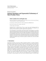
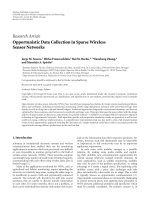
The scenario of interest for this work is shown in
Figure 1. The primary system consists of a single transmitter

located at a distance of d
0
from its intended receiver. Without
any loss of generality, the primary receiver is considered to be
located at the origin of the coordinates system, leading to a
receiver-centric analysis. The secondary (cognitive) terminals
are deployed along with the primary ones. However, limita-
tions on interference prevent them from entering a protected
region around the receiver. This region, referred to as the
“primary exclusive region” [21], is assumed to be circular and
therefore, is completely characterized by its radius, denoted
as d
excl
.
Since polarimetric diversity does not allow a perfect
orthogonality between primary and secondary nodes’ trans-
missions, its use is possible under the application of a so-
called underlay paradigm [10, 22, 23]. This means that both
cognitive and primary terminals carry out communications,
provided that the capacity loss caused by cognitive users
does not degrade communication quality for primary users.
For this purpose, we can further characterize the underlaid
paradigm by requiring that the primary system must be
guaranteed a minimum (transmission) capacity during a
large fraction of time. As will be shown, this can, in turn,
be formulated as a probabilistic coexistence problem under
the constraint of a limited outage probability in the primary
network.
We argue that using the polarimetric dimension allows
dynamic spectrum sharing to be efficiently implemented

in cognitive systems. To this end, we propose a theoreti-
cal model of interference in dual-polarized networks and
derive a closed-form expression for the link probability of
outage. We theoretically prove that polarimetric diversity
can increase transmission rates for the secondary terminals
while, at the same time, can significantly reduce the primary
exclusive region.
First, we validated the expected (theoretical) perfor-
mance gains analytically. To the best of our knowledge, none
of the past studies in literature has investigated the behavior
of the XPD under a complete range of propagation con-
ditions, such as indoor-to-indoor and outdoor-to-indoor.
In particular, we conducted a vast experimental campaign
to provide relevant insights on the proper models and
statistical distributions which would accurately represent the
XPD. Based on these measures, the achievable performance
of these dual-polarized cognitive networks, considering
both half-duplex and full-duplex communications, will be
determined.
The medium access control (MAC) protocol considered
is a variant of the slotted ALOHA protocol [24] such that
in each time slot, the nodes transmit independently with a
Cognitive
terminals
Primary
terminal
Cognitive
terminals
Primary exclusive region
d

excl
d
0
Figure 1: Cognitive network model: a single primary transmitter is
placed at the center of a primary exclusive region (PER), with radius
d
excl
, where its intended receiver is present.
certain fixed probability [25]. This approach is supported
by the observations in [26, page 278] and [25, 27], where it
is shown that the traffic generated by nodes using a slotted
random access MAC protocol can be modeled by means
of a Bernoulli distribution. In fact, in more sophisticated
MAC schemes, the probability of transmission of a terminal’s
transmission can be modeled as a function of general
parameters, such as, queuing statistics, the queue-dropping
rate, and the channel outage probability incurred by fading
[28]. Since the impact of these parameters is not the focus of
the this study, for more details we refer the interested reader
to the existing studies in the literature [29–31].
The remainder of this paper is organized as follows. In
Section 2, we demonstrate how the polarimetric dimension
increases spectrum-utilization efficiency and supports the
coexistence of primary and secondary users in a probabilistic
sense, which requires guaranteed capacity for the pri-
mary network. After these theoretical developments, several
insights are presented to move from the concept to practical
implementation. First, Section 3 presents an experimental
determination of the main parameters used to characterize
cognitive dual-polarized networks in indoor-to-indoor and

outdoor-to-indoor situations. These results are then used
in Section 4 for analytical performance evaluation. Section 5
concludes the paper.
2. The Dual-Polarized Cognitive
Network Architecture
2.1. Probabilistic Coexistence and Interference. Consider the
cognitive network shown in Figure 1 with two types of users:
primary and secondary (cognitive). The primary network
is supposed to be copolar and the cognitive network is
cross-polar. Without cognitive users, the primary network
would operate with background noise and with the usual
interference generated by the other primary users. Let C
p
(dimension: [bit/s/Hz]) be the desired capacity for a user in
the primary network (In this manuscript, bold letters refer
to random variables). We impose that the secondary network
EURASIP Journal on Wireless Communications and Networking 3
operates under the following outage constraint on a primary
user:
P

C
p
≤ C

≤
ε,(1)
where 0 <ε<1andC (dimension: [bit/s/Hz]) is a mini-
mum per-primary user capacity. Equivalently, this constraint
guarantees a primary user a maximum transmission rate of

at least C for at least a fraction (1
− ε) of the time. Under the
simplifying assumption of Gaussian signaling (Note that this
assumption is expedient for analytical purposes. However, in
the following the analytical predictions will be confirmed by
experimental results.), the rate of this primary user can be
written as a function of the signal-to-noise and interference
ratio (SINR) as follows:
C
p
= log
2
(
1+SINR
)
.
(2)
Using (2) into (1) yields
P

C
p
≤ C

≤
ε ⇐⇒ P

log
2
(

1+SINR
)
≤ C

≤
ε
⇐⇒ P

SINR ≤ 2
C
− 1

≤
ε
(3)
and, by introducing θ  2
C
− 1, one has
P

C
p
≤ C

≤
ε ⇐⇒ P{SINR >θ} > 1 − ε,(4)
where
P{SINR >θ} can be interpreted as the primary link
probability of successful transmission for an outage SINR
value θ. This value depends on the receiver’s characteristics,

modulation, and coding scheme, among others [32]. The
SINR at the end of a primary link with length d
0
can be
written as
SINR 
P
0
(
d
0
)
N
0
B+P
int
,
(5)
where P
0
(d
0
) is the instantaneous received power (dimen-
sion: [W]) at distance d
0
, N
0
/2 is the noise power spectral
density of the noise (dimension: [W/Hz]), B is the channel
bandwidth, and P

int
is the cumulated interference power
(dimension: [W]) at the receiver, that is, the sum of the
received powers from all the undesired transmitters. We now
provide the reader with a series of theoretical results, which
stem from the following theorem.
Theorem 1. In a narrowband Rayleigh block-faded dual-
polarized network, where nodes transmit with probability q on
the copolar and the cross-polar channels, the probability that
the SINR exceeds a given value θ on a primary transmission,
given a fixed transmitter-receiver distance d
0
, N

int
copolar
interferers at distances
{d
i
}
N

int
i=1
transmitting at powers {P

i
}
N


int
i=1
,
and N
⊥
int
cross-polar interferers at distances {d

j
}
N
⊥
int
j=1
trans-
mitting at powers
{P
⊥
j
}
N
⊥
int
j=1
w ith a cross-polar discriminat ion
coefficient XPD
0
,is
P{SINR >θ}
=

exp

−
θ
N
0
B
P
0
d
−α
0

×
N

int

i=1
⎧
⎨
⎩
1 −
θq

P
0
/P

i


(
d
i
/d
0
)
α
+ θ
⎫
⎬
⎭
×
N
⊥
int

j=1
⎧
⎪
⎨
⎪
⎩
1 −
θq
XPD
0
G
(
d, d

ref
)

P
0
/P
⊥
j

d

j
/d
0

α
+ θ
⎫
⎪
⎬
⎪
⎭
,
(6)
where P
0
is the transmit power, N
0
B is the average power of
the background noise, θ is the SINR threshold, α is the path

loss exponent, XPD
0
is the reference cross-polar discrimination
of the antenna at a reference distance d
ref
,andG(d, d
ref
) is a
function that characterizes the polarization loss over distance.
Proof. We assume a narrowband Rayleigh block fading
propagation channel. The instantaneous received power P(d)
from a node is exponentially distributed [33]withtemporal-
average received power
E
t
[P(d)] = P(d) = P · L(d), where P
denotes the transmit power and L(d)
∝ d
−α
is the path loss
at distance d (it accounts for the antenna gains and carrier
frequency). The received power is then a random variable
with the following probability density function:
f
P
(
x
)
=
1

P
(
d
)
exp

−
x
P
(
d
)

=
1
P · L
(
d
)
exp

−
x
P · L
(
d
)

.
(7)

In a dual-polarized system, the cross-polar discrimination
(XPD) is defined as the ratio of the temporal-average power
emitted on the cross-polar channel and the temporal-average
power received in the copolar channel [15], that is,
P
(⊥→)
(
d
)
=
P
⊥
(
d
)
XPD
(
d
)
,
(8)
where d is the transmission distance, P
(⊥→)
j
(d) 
E
t
[P
(⊥→)
(d)] is the temporal-average value of the instan-

taneous leaked power P
(⊥→)
(d), and P
⊥
(d)  E
t
[P
⊥
(d)]
is the temporal-average value of the instantaneous cross-
polar power P
⊥
(d). In a generic situation, the XPD is subject
to spatial variability [19] and, therefore, in the context of
this network-level analysis, we define the XPD in a spatial-
average sense, that is,
XPD
(
d
)


P
⊥
(
d
)
P
(⊥→)
(

d
)

,
(9)
where the operator
X denotes the average of the value
X computed on multiple different locations at the same
distance d. Note that, even though the XPD is considered
here in a spatial-average sense, it is possible to accommodate
its expected variability for the purpose of ensuring a required
minimum cross-polar discrimination. This will be detailed
4 EURASIP Journal on Wireless Communications and Networking
in Section 4. Finally, it is shown in [17–19], that XPD(d),
defined according to (9), can be expressed as follows:
XPD
(
d
)
= XPD
0
G
(
d, d
ref
)
,
(10)
where XPD
0

≥ 1 is the XPD value at a reference distance
d
ref
and the function G(d, d
ref
) ≤ 1 characterizes the de-
polarization experienced over the distance.
Let the traffic at the N

int
primary and N
⊥
int
cognitive inter-
fering nodes be modeled through the use of independent
indicators
{Λ
i
}
N

int
i=1
, {Λ

j
}
N
⊥
int

j=1
,withforalli, j; Λ
i
, Λ

j
∈{0, 1}.
In other words,
{Λ
i
} and {Λ

j
} are sequences of independent
and identically distributed (iid) Bernoulli random variables:
if, in a given time slot, one of these indicators is equal to
1, then the corresponding node is transmitting; if, on the
other hand, the indicator is equal to 0, then the node is not
transmitting. We also assume that the traffic distribution is
the same at all interfering nodes of the network, that is, for
all i,
P{Λ
i
= 1}=q and for all j, P{Λ

j
= 1}=q,which
is supported by the analyses presented in [25, 27, 34]. The
overall interference power at the receiver is the sum of the
interference powers due to copolarized and cross-polarized

(leaked because of depolarization) interference powers, that
is,
P
int
=
N

int

i=1
P

i
(
d
i
)
Λ
i
+
N
⊥
int

j=1
P
(⊥→)
j

d

j

Λ

j
,
(11)
where
{P

i
(d
i
)} and {P
(⊥→)
j
(d
j
)} are the (instantaneous)
interfering powers at the receiver. The probability that the
SINR at the receiver exceeds θ can thus be expressed as
follows:
P{SINR >θ}
= E
P
int
[
P{SINR >θ}|P
int
]

= E
{P

i
},{Λ
i
},{P
(⊥→)
j
},{Λ

j
}
×
⎡
⎢
⎣
exp
⎛
⎜
⎝
−
θ
P
0
L
(
d
0
)

×
⎛
⎜
⎝
N
0
B +
N

int

i=1
P

i
(
d
i
)
Λ
i
+
N
⊥
int

j=1
P
(⊥→)
j


d
j

Λ

j
⎞
⎟
⎠
⎞
⎟
⎠
⎤
⎥
⎦
=
exp

−
θ
N
0
B
P
0
L
(
d
0

)

× E
{P

i
},{Λ
i
},{P
(⊥→)
j
},{Λ

j
}
×
⎡
⎢
⎣
N

int

i=1
exp

−
θP
i


(
d
i
)
Λ
i
P
0
L
(
d
0
)

×
N
⊥
int

j=1
exp
⎛
⎝
−
θP
(⊥→)
j

d
j


Λ

j
P
0
L
(
d
0
)
⎞
⎠
⎤
⎥
⎦
,
(12)
where in the second passage, we have exploited the fact
that, in a Rayleigh faded transmission, the SINR is also
exponentially-distributed [33]. Since all terminals have an
independent transmission behavior and are subject to non-
correlated channel fading, that is,
{P

i
}, {Λ
i
}, {P
(⊥→)

j
},and
{Λ

j
} are independent sets of random variables, it then holds
that
P{SINR >θ}
=
exp

−
θ
N
0
B
P
0
L
(
d
0
)

×
N

int

i=1

E
{P

i
},{Λ
i
}

exp

−
θP

i
(
d
i
)
Λ
i
P
0
L
(
d
0
)

×
N

⊥
int

j=1
E
{P
(⊥→)
j
},{Λ

j
}
⎡
⎣
exp
⎛
⎝
−
θP
(⊥→)
j

d
j

Λ

j
P
0

L
(
d
0
)
⎞
⎠
⎤
⎦
.
(13)
The generic first expectation term at the right-hand side of
(13) can be expressed as follows:
E
{P

i
},{Λ
i
}

exp

−
θP

i
(
d
i

)
Λ
i
P
0
L
(
d
0
)

= P{
Λ
i
= 1}×

∞
0
exp

−
θp
i
P
0
L
(
d
0
)


f
P

i

p
i

dp
i
+ P{Λ
i
= 0}×1
= 1 −
θq

P
0
/P

i

(
d
i
/d
)
α
+ θ

.
(14)
The generic second expectation term in (13)canbe
expressed, by using (8), in a similar way:
E
{P
(⊥→)
j
},{Λ

j
}
⎡
⎣
exp
⎛
⎝
−
θP
(⊥→)
j

d
j

Λ

j
P
0

L
(
d
0
)
⎞
⎠
⎤
⎦
= P

Λ

j
= 1

×

∞
0
exp

−
θp
j
P
0
L
(
d

0
)

f
P
(⊥→)
j

p
j

dp
j
+ P

Λ

j
= 0

×
1
= 1 −
θq
XPD
0
G
(
d, d
ref

)

P
0
/P
⊥
j

d

j
/d
0

α
+ θ
.
(15)
By plugging (14)and(15) into (13), one finally obtains
expression (6) for the probability of successful transmis-
sion.
Theorem 1 gives interesting insights on the expected
performance in a dual-polarized transmission subject to
background and internode interference. First, the leftmost
term of the expression at the right-hand side of (6)is
relevant in a situation where the throughput is limited by the
EURASIP Journal on Wireless Communications and Networking 5
background (typically thermal) noise. In large and/or dense
networks, the transmission is only limited by the interference
and one can focus on the interference and polarization terms

(i.e., the two other term of the expression, assuming N
0
B is
negligible). The first exponential term can be easily evaluated
if N
0
B
/
= 0.
The second and the third terms of expression (6)relate
to the interference generated by the surrounding nodes
transmitting in co- and cross-polarized channels. These
terms depend on (i) the polarization characteristics of the
interfering nodes, (ii) the traffic statistics, and (iii) the
topology of the network. Note that the impact of the
topology has been largely investigated in [35]andwewill
limit our study to the effect of polarization.
Finally, channel correlation is neglected here, as often in
the literature, for the purpose of analytical tractability and
because these correlations do not change the scaling behavior
of link-level performance. For the sake of completeness, we
note that in [36] an analysis of the impact of channel cor-
relation is carried out. The authors conclude that, when the
traffic is limited (q<0.3), the assumption of uncorrelation
holds. On the other hand, when the traffic is intense (q
≥
0.3), the link probability of success is higher in the correlated
channel scenario than in the uncorrelated channel scenario.
2.2. Probabilistic Link Throughput. Referring back to our
definition of the probabilistic coexistence of the primary

and secondary terminals in (1), a transmission is said to
be successful if and only if the primary terminal is not in
an outage for a fraction of time longer than (1
− ε), that
is, if the (instantaneous) SINR of the cognitive terminal is
above the threshold θ. Therefore, we denote the probability
of successful transmission in a primary link as P
s
, that is,
P
s
= P{SINR >θ}.
(16)
The probabilistic link throughput [37](adimensional)ofa
primary terminal is defined as follows:
(i) in the full-duplex communication case, it corre-
sponds to the product of (a) P
s
and (b) the proba-
bility that the transmitter actually transmits (i.e., q);
(ii) in the half-duplex communication case, it corre-
sponds to the product of (a) P
s
, (b) the probability
that the transmitter actually transmits (i.e., q), and
(c) the probability that the receiver actually receives
(i.e., 1
− q).
The probabilistic link throughput can be interpreted as
the unconditioned reception probability which can be

achieved with a simple automatic-repeat-request (ARQ)
scheme with error-free feedback [38]. For the slotted ALOHA
transmission scheme under consideration, the probabilistic
throughput in the half-duplex mode is then τ
(half)
 q(1 −
q)P
s
and in full-duplex case τ
(full)
 qP
s
.
2.3. Properties and Opportunities of Polarization Diversity.
Theorem 1 expresses a network-wide condition to support
the codeployment of primary and cognitive terminals. In
order to implement polarization diversity and make it work,
proper considerations have to be carried out. In this section,
we propose several lemmas, all derived from Theorem 1, that
allow to design and operate dual-polarized systems.
Lemma 2. In a dual-polarized system subject to probabilistic
coexistence of primary and secondary networks, relocating a
cognitive terminal from the copolar channel to the cross-polar
channel increases its probability of transmission while keeping
intact the transmission capacity of the primary net work.
Proof. Let us consider a scenario with a single interferer
located at distance d and transmitting with power P. For the
ease of understanding, let us assume that if the terminal uses
a polarized antenna, its probability of transmission will be
denoted as q

= q
⊥
, whereas if a classical (not dual-polarized)
scenario is considered, then q
= q

.
If the cognitive terminal is using the copolar mode, the
probabilistic coexistence condition (1)canbewrittenas
θq

(
P
0
/P
)(
d/d
0
)
α
+ θ
≤ ε;
(17)
whereas if the cognitive terminal is using the cross-polar
mode, it holds that
θq
⊥
XPD
(
d

)(
P
0
/P
)(
d/d
0
)
α
+ θ
≤ ε.
(18)
Therefore, the maximum acceptable probability of transmis-
sion in the copolar mode is
q

max
= ε

1+
1
θ
P
0
P

d
d
0


α

. (19)
Note that, on average, XPD(d)
≥ 1 according to definition
(8) and for physical reasons—the power leaked on the
copolar dimension is at most equal to the power transmitted
on the cross-polar channel. Finally, all other quantities in
(19) are strictly positive and, therefore, one obtains that
q

max
≤ ε

1+
XPD
(
d
)
θ
P
0
P

d
d
0

α


=
q
⊥
max
, (20)
where the right-hand side expression for q
⊥
max
derives directly
from (18). Therefore, the thesis of the lemma holds.
Lemma 2 indicates that polarization can be exploited as
a diversity technique. Indeed, the achievable transmission
rate will always be increased if the secondary network uses
a polarization state that is orthogonal to that of the primary
network and, furthermore, this remains true regardless of
the values taken by the other system parameters (e.g.,
transmission power, acceptable outage rate ε, SINR value,
etc.).
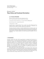
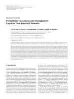
Lemma 3. There exists a region of space, referred to as the
primary exclusive region, where the cognitive terminals are
not allowed to transmit and can be reduced by means of
polarimetric diversity.
6 EURASIP Journal on Wireless Communications and Networking
No polarization
XPD
0
= 4dB
XPD
0
= 8dB

XPD
0
= 10dB
00.20.40.60.81
1
2
3
4
q
d
excl
/d
0
Figure 2: Primary exclusive region as a function of the terminal
probability of transmission q, for various polarimetric values and
with ε
= 0.2.
Proof. As previously anticipated in Section 1, the primary
exclusive region is completely characterized by the primary
exclusive distance d
excl
, that is, the minimum distance at
which a cognitive terminal has to be, with respect to a
primary receiver, so that it does not impact the capacity of
the primary user (in a probabilistic sense) [21]. Starting from
(6), in the presence of a single cross-polar interferer, one can
write
θq
XPD
(

d
)(
P
0
/P
)(
d/d
0
)
α
+ θ
≤ ε.
(21)
This relation is equivalent to
d
d
0
≥

1
XPD
0
G(d, d
ref
)

1/α

θ
P

P
0
q − ε
ε

1/α

d
excl
d
0
,
(22)
where the definition at the right-hand side allows to express
the minimum distance d
excl
as a function of the distance d
0
and the other main system parameters as follows:
d
excl
= d
0

1
XPD
0
G(d, d
ref
)


1/α

θ
P
P
0
q − ε
ε

1/α
.
(23)
Therefore, since α
≥ 2, using polarization diversity, that is,
causing XPD
0
G(d, d
ref
) > 1, reduces d
excl
.
In Figure 2, the normalized primary exclusive distance,
defined as d
excl
/d
0
, is shown, as a function of the terminal
probability of transmission q,withε
= 0.2. It can be observed

that in the case without polarization, one always has d
excl

d
0
, that is, the cognitive terminals must be located outside the
transmission zone defined by the primary emitter-receiver
distance. On the opposite, it is possible to operate a cognitive
terminal inside this region (i.e., with d
excl
<d
0
) when the
polarimetric dimension is used. Furthermore, in both cases
the exclusive distance increases as a function of the terminal
probability of transmission but its gradient is smaller in the
dual-polarized case.
It is interesting to observe that relation (21) can also be
used to parameterize practical realizations of the antennas.
Indeed, it yields that
XPD
(
d
)
≥
P
P
0

d

0
d

α

q − ε

ε
θ
(24)
from which, with XPD(d)
= XPD
0
G(d, d
ref
), it follows that
XPD
0
≥
1
G
(
d, d
ref
)
P
P
0

d

0
d

α

q − ε

ε
θ.
(25)
Therefore, the quantity at the right-hand side of (25)
represents the minimum amount of XPD that the antenna of
the cognitive terminal must possess. This value depends on
the network configuration but also on the propagation envi-
ronment (through the depolarization function G(d, d
ref
)).
Lemma 4. If q<ε, polarizat ion diversity is not required to
achieve a probabilistic c oexistence.
Proof. As previously introduced, the coefficient XPD
0
is
greater than or equal to 1. Therefore, the minimum value
of XPD
0
to guarantee error-free transmissions on the cross-
polar channel is
XPD
0
= max


1,
1
G
(
d, d
ref
)
P
P
0

d
0
d

α

q − ε

ε
θ

. (26)
In (25), all quantities are greater than zero. Therefore, if q<
ε, the quantity q
− ε is always negative and the solution of
(26)isXPD
0
= 1.

Lemma 4 indicates that, if the desired throughput
remains limited, then the outage is guaranteed on the
primary system without summoning up the diversity of
polarization on the secondary terminal. Therefore, the cross-
polar channel can be kept available for other terminals that
may require higher data rates. This can be observed in
Figure 2.
Theorem 5. Besides being limited by probabilistic coexistence
considerations, there exists an optimum probability of trans-
mission by a terminal in the primary network, denoted as q
opt
,
that maximizes the throughput.
Proof. Let us define the optimal user probability of transmis-
sion as
q
opt
 arg max
q
τ,
(27)
where the probabilistic throughput τ has been defined in
Section 2.2. We first focus on half-duplex systems, using
polarization diversity: in this case, the link throughput is
τ
= q(1 − q)P
s
. Since ln(·) is a monotonically increasing
function, finding the maximum of τ is equivalent to finding
the maximum of ln(τ), that is,

q
opt
= arg max
q
ln
(
τ
)
.
(28)
EURASIP Journal on Wireless Communications and Networking 7
In order to find the maximum, we compute the partial
derivative of ln(τ)withrespecttoq:
∂
∂q
ln
(
τ
)
=
1
q
−
1
1 − q
+
∂
∂q
N
⊥

int

j
ln

1 −
q
η
j

,
(29)
where
η
j

XPD
0
θ
G
(
d, d
ref
)
P
0
P
⊥
j


d

j
d
0

α
+1.
(30)
By using the approximation (This approximation is accurate
for 0 <q<η
j
/3, which is always verified since d

j
and XPD
0
need to be kept high because of the probabilistic coexistence
constraint.) ln(1 + x)
≈ x and setting ∂ ln(τ)/∂q = 0, one has

q
opt

2
− q
opt

1+2η


+ η ≈ 0,
(31)
where η  1/

N
⊥
int
j
η
−1
j
. The positive solution of this equation
is given by
q
opt
≈ η +
1
2

1 −

1+4η
2

(32)
which is the probability of transmission that maximizes the
throughput. The same derivation can be applied in the case
of a full duplex system and leads to the solution q
opt
≈ η.If

the approximation ln(1+x)
≈ x is not used, then the optimal
probability of transmission cannot be given in a closed-form
expression but has to be numerically evaluated.
Obviously, the maximum value of q will be the minimum
between (i) the optimum probability of transmission in
a slotted transmission system (in a general sense), given
by (32), and (ii) the maximum rate that can be achieved
under the constraint of a probabilistic coexistence in (20).
Therefore, before selecting its transmission rate, a cognitive
terminal must evaluate these two quantities, on the basis of
the available information stored in the databases (positions
of the nodes, acceptable outage, etc.), and use the smallest
one.
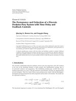
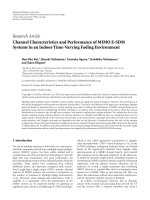
In Figures 3(a) and 3(b), the accessible and optimal
terminal probabilities of transmission are presented as
functions of d/d
0
, in the cases with (a) half duplex and (b)
full duplex communications, respectively. In each case, two
polarization strategies are considered: (i) no polarization
and (ii) XPD
0
= 10 dB. The accessible regions are defined
by means of the inequality (22). In particular, the leftmost
border of each exclusive region, denoted as line q
excl
,is
defined as the probability of transmission for a terminal at
the boundary of the primary exclusive region, that is, with

d
= d
excl
.
From these figures, it can be observed that the probability
of transmission of dual-polarized cognitive systems is mainly
limited by the interference bound imposed to protect the pri-
mary system. In fact, the transmission rate of the terminals
will nearly always be lower than the optimal transmission
rate, except when the cognitive terminal is distant. In that
specific case, the optimum probability of transmission (20)
in the accessible region (in a probabilistic sense) saturates,
that is, it reaches q
opt
≈ 1/2 in the half-duplex case and q
opt
≈
1 in the full-duplex case. Note that these values correspond
to the maximum achievable throughput observed in any
half-duplex or full-duplex system. Indeed, the definitions of
the probabilistic link throughput are τ
(half)
 q(1 − q)P
s
and τ
(full)
 qP
s
and the corresponding optimum terminal
probabilities of transmission cannot exceed q

= 1/2and
q
= 1, respectively.
In the scenarios where polarimetric diversity is exploited,
this crossover distance is smaller (d
excl
/d
0
≈ 1.5) than in
the classical case (d
excl
/d
0
≈ 3.3). Comparing the results in
Figure 3(a) with those in Figure 3(b), another observation
can be carried out. In the half-duplex case, for each distance
d>d
excl
, the optimal transmission probability q
opt
lies
inside the accessible region. In other words, q has to be
properly selected to maximize the throughput. In the full-
duplex case, q
opt
≈ 1 everywhere in the exclusive region.
These observations will be confirmed by the results presented
in Section 4.
Finally, it is confirmed that, in the accessible regions, one
either has (i) (d


j
/d
0
)
α
 1withXPD
0
> 1(i.e.,q/η
j

1) or (ii) q
opt
 0.3. Therefore, the approximation used in
proof of Theorem 5 (i.e., ln(1 + x)
≈ x) holds and the value
of q
opt
derived in Theorem 5 canbeconsideredasanaccurate
approximation of the true value.
2.4. Considerations for Practical System Implementation. In
the previous subsections, we have shown that the capacity
of a primary user can be guaranteed, while, at the same
time, allowing efficient spectrum access, if the polarimetric
dimension is exploited. Moreover, dual-polarized terminals
will benefit from an increase of capacity by means of a
higher transmission rate and reduced terminal-to-terminal
interference. The efficiency of polarization diversity depends
on the cross-polar discrimination of the antennas in use.
More precisely, the value of the initial cross-polar discrim-

ination (i.e., XPD
0
) has to be as high as possible; yet, the
XPD of well-designed antennas is typically on the order of
10
÷ 20 dB [15, 39], which allows a significant discrimination
between copolar and cross-polar channels. Depending on
the achievable value of XPD
0
, the outage rate of a primary
terminal, and the location of the terminals, the transmission
rate of a cognitive terminal can be adapted taking into
account the relations (20)and(32). Finally, the primary
exclusive region can be determined by means of (22)and
notified to the cognitive terminals which, in turn, can use it
as a constraint.
3. Experimental Determination of
the Indoor-to-Indoor and
Outdoor -to-Indoor XPD
Severalpreviousworkshavebeenundertakeninorderto
model the XPD for different kinds of environment. In [20], a
theoretical analysis is conducted for the small-scale variation
of XPD in an indoor-to-indoor scenario and it is concluded
that it has a doubly, noncentral Fisher-Snedecor distribution.
8 EURASIP Journal on Wireless Communications and Networking
01234
0.2
0.4
0.6
0.8

1
d/d
0
q
q
excl
q
opt
q
opt
q
excl
XPD
0
= 10dB
No polarization
Accessible region
(a) Half duplex communications
01234
0.2
0.4
0.6
0.8
1
d/d
0
q
q
excl
q

opt
q
opt
q
excl
XPD
0
= 10dB
No polarization
Accessible region
(b) Full duplex communications
Figure 3: Accessible and optimal terminal probabilities of transmission as a function of d/d
0
and for ε = 0.1. In both cases, two polarization
strategies are considered: (i) no polarization (drawn in red) and (ii) polarization with XPD
0
= 10 dB (drawn in blue).
A mean-fitting (i.e., the pathloss) model of XPD as a
function of the distance in an outdoor-to-outdoor scenario
was studied in [16, 19]. The corresponding performance is
analyzed in [11].
In this paper, we provide the reader with original
measurements campaigns in both indoor-to-indoor and
outdoor-to-indoor scenarios. Indeed, these correspond to
real-life situations where various technologies, such as WiFi,
sensor networks, personal area networks (indoor-to-indoor
scenarios) or WiMax, public WiFi, and 3G systems (outdoor-
to-indoor scenarios) are in use.
We consider three generic models to describe the varia-
tion of the XPD with respect to the distance. For instance,

when the transmission ranges are long (several hundreds of
meters or a few kilometers), the best expression for the path
loss function is
G
1
(
d, d
ref
)
=

d
d
ref

−β
,
(33)
where β is a decay factor (0 <β
≤ 1). On the other
hand, when distances are small (tens of meters) or in indoor-
to-indoor scenarios, the XPD value, in decibels, decreases
linearly with respect to the distance. In other words, one can
write
XPD
(
d
)
[
dB

]
= XPD
0
[
dB
]
− γd
(34)
which corresponds, in linear scale, to the following path loss
function:
G
2
(
d, d
ref
)
= 10
−(γ/10)d
.
(35)
Finally, in some indoor scenarios where the transmission
distances are small, it was observed that the XPD remains
constant, that is,
G
3
(
d, d
ref
)
= 1.

(36)
In the remainder of this section, we characterize the
applicability of the three XPD models just introduced. In
other words, we consider an experimental setup and, on the
basis of an extensive measurement campaign, we determine
which XPD model is to be preferred in each scenario of
interest (indoor-to-indoor and outdoor-to-indoor).
3.1. Setup. The measurements were performed using a
Vector Signal Generator (Rohde & Schwarz SMATE200A
VSG) at the transmitter (Tx) side and a Signal Analyzer
(Rohde & Schwarz FSG SA) at the receiver (Rx) side. The Tx
chain was composed of the VSG and a directional antenna.
The Rx antenna was a tri-polarized antenna, made of three
colocated perpendicular antennas. Two of these antennas
were selected to create a Vertical-Horizontal dual-polarized
antenna. The three receiver antennas were selected one after
another by means of a switch and were connected to the
Signal Analyzer through a 25 dB, low-noise amplifier. The Rx
antennas were fixed on an automatic positioner to create a
virtual planar array of antennas. A continuous wave (CW)
signal at the frequency of 3.5 GHz was transmitted and
the corresponding frequency response was recorded at the
receiver side. The antenna input power was 19 dBm.
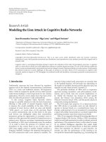
The measurement site was the third floor of a building
located on the campus of Brussels University (ULB) and
referred to as “Building U.” In the outdoor-to-indoor case,
shown in Figure 4(a), the transmitter was fixed on the
rooftop of a neighboring building (referred to as “Building
L”), at a height of 15 m and was directed toward the
measurement site. A brick wall was separating the line-

of-sight (LOS) direction between this measurement site
and the transmitter. The measurements were performed
in a total of 78 distinct locations and in seven successive
rooms. The rooms were separated by brick walls and closed
wooden doors. The distance between the transmitter and
the measurement points was in the range between 30 m and
80 m. In the indoor-to-indoor case, shown in Figure 4(b),
the Tx antenna was fixed in the first room and was directed
toward the seven next rooms, in which 65 measurement
points were considered. The distance between the transmitter
EURASIP Journal on Wireless Communications and Networking 9
and the measurement points was in the range between 8m
and 55 m. In order to characterize the small-scale statistics
of XPD a total of 64 spatially separated measurements were
taken at each Rx position and in an 8
× 8 grid. The spacing
between grid points was λ/2
= 4 cm. At each grid point, 5
snapshots of the received signal were sampled and averaged
to increase the signal-to-noise-ratio.
3.2. Experimental Results and Their Interpretation. The anal-
ysis of the collected experimental results has shown that the
values of the XPD, for a given distance, present a location-
dependent variability. Therefore, in the following figures,
where the XPD is shown as a function of the distance d,
the average value is shown along with the 1σ and 2σ being
confidence intervals. Since the spatial variations were found
to be Gaussian, these intervals account for 68% and 95% of
the observed sets, respectively.
The horizontal polarization was first used in an indoor-

to-indoor scenario and is reported in Figure 5.Itwas
observed that the XDP can be accurately modeled by
means of the propagation model G
2
(d, d
ref
)whereonehas
XPD
0
= 11.3dB, d
ref
= 1m, and γ = 0.16 dB/m. The
variation around the average value was also analyzed and
the corresponding cumulative distribution function (CDF) is
shown in Figure 6. This variation was found to fit with a zero-
mean Gaussian random variable with standard deviation
equal to 0.295 dB. It is interesting to note that, unlike the
case of the outdoor-to-outdoor scenarios presented in [19],
the behavior of the XDP depends on the initial polarization
of the antenna. More precisely, the results in Figure 6
correspond to a horizontal polarization while the results in
Figure 7 correspond to an initial vertical polarization. It can
be seen that, in the latter scenario, the XPD is almost constant
and equal to XPD
0
= 4 dB. In this case, the XPD variability
can be modeled as a zero-mean Gaussian random variable
with standard deviation equal to 2.75 dB.
Finally, the results collected in an outdoor-to-indoor
scenario are presented in Figure 8.Asexpected,theXPDisa

decreasing function of the distance and is suitably modeled
by using the propagation model G
2
(d, d
ref
), with XPD
0
=
12.87 dB, d
ref
= 20 m, and γ = 0.13 dB/m. The spatial
variability can be modeled as a zero-mean Gaussian random
variable with standard deviation equal to 2.95 dB. Note that
full de-polarization occurs after a hundred of meters and the
two initial polarizations (i.e., horizontal and vertical) lead to
the same behaviour.
4. Numerical Performance Evaluation
In this section, a numerical analysis of the performance of
the proposed dual-polarized cognitive systems is presented.
In Section 3, it has been shown that the XPD experiences
spatial shadowing: more precisely, at a fixed distance different
values of the XPD can be observed at different locations.
The system parameters for performance analysis are selected
by taking into account this normal fluctuation. Therefore,
instead of using the average value for XPD
0
,itispreferableto
useavalue(denotedasXPD
min
0

) that can be observed with a
confidence equal to a predefined value δ
∈ (0, 1). Taking into
account that XPD
0
has a Gaussian distribution, it follows that
P

XPD
0
≤ XPD
min
0

=
1 − Q

XPD
min
0
− μ
σ

=
δ,
(37)
where μ and σ are the average value and the standard
deviation of the observed XPD
0
, respectively. Therefore,

XPD
min
0
can be expressed as
XPD
min
0
= μ + σQ
−1
(
δ
)
.
(38)
For instance, if a confidence level of 80% is required (i.e., δ
=
0.8), one has to select XPD
min
0
= μ − σQ
−1
(0.8) ≈ μ − 0.81σ.
This approach will be used to set the initial parameters in the
following performance analysis.
4.1. Full Duplex Systems in an Outdoor-to-Indoor Scenario.
Cellular system typically corresponds to an outdoor-to-
indoor scenario. Examples include WiMax base stations or
cellular mobile phone systems. A typical scenario is presented
in Figure 9. Referring to the experimental results presented in
Section 3, we used in our simulations the model G

1
(d, d
ref
)
with parameters α
= 3, β = 0.4, and XPD
0
= 4 ÷ 10 dB. Also,
the measurements lead us to set XPD
min
0
equal to 10.48 dB
with an 80% confidence level. The cell radius is r
= 200 m, 10
cognitive terminals are deployed, their distances uniformly
distributed over [0, r]. Finally, the Tx-Rx distance in the
primary network is d
0
= 30 m.
Two d ifferent polarization strategies are investigated:
(i) the primary and the cognitive networks do not use
polarimetric diversity (this scenario is referred to as no
polarization) and (ii) the systems reduce their interference
by using two orthogonal polarization states (this scenario is
referred to as full polarization).
In Figure 11, the performance of full duplex systems is
presented. More specifically, in Figure 11(a), the throughput
of the system is shown as a function of the terminal proba-
bility of transmission. It can be seen that the throughput of
the dual-polarized system is significantly higher, particularly

when the probability of transmission is high. In Figure 11(b),
the corresponding link probability of success in the primary
network is investigated. It can be seen that it confirms the
conclusions of Lemma 2: for a given minimum value of
the link probability of success, the achievable transmission
rate is significantly higher in the dual-polarized mode with
respect to the value observed with the classical approach. For
instance, with ε
= 0.8, one has q
max
= 0.15 while, by using
the dual-polarized approach, the maximum probability of
transmission can be increased up to q
max
= 1.0. In other
words, virtually any transmission rate is achievable with a
limited impact on the primary system.
4.2. Half-Duplex System in an Indoor-to-Indoor Scenario. In
a second scenario, the probabilistic coexistence is analyzed in
the context of half-duplex systems, where indoor-to-indoor
transmissions are typically used. Examples include wireless
sensor networks (WSNs), ZigBee systems, and body area net-
10 EURASIP Journal on Wireless Communications and Networking
Rx
Tx
Window glasses
Wooden door
Building U,
third floor
62 m

15 m
(a) Indoor-to-indoor measurement setup
Window glasses
Wooden door
Building L rooftop
Building U,
third floor
53 m
11 m
15 m
27 m
Rx
Tx
(b) Outdoor-to-indoor measurement setup
Figure 4: Scenario descriptions.
0 102030405060
−5
0
5
10
15
20
d
XPD (dB)
Figure 5: XPD in logarithmic scale, as a function of the Tx
distance, in the indoor-to-indoor scenario with an initial horizontal
polarization.
works (BANs). A typical scenario is presented in Figure 10.
In our simulations, we considered a primary transmission
at distance d

0
= 15 m and subject to interference from 5
terminals located at d
= 25 m from the central base station.
−4 −20 2 4 6 810
0
0.1
0.2
0.3
0.4
0.5
0.6
0.7
0.8
0.9
1
x (dB)
P{XPD ≤ x}
Figure 6: CDF of the XPD in the indoor-to-indoor scenario.
This corresponds to d/d
0
≈ 1.67 and it can be seen from
Figure 3(a) that this value is in the accessible region. The
propagation model G
3
(d, d
ref
) is used and the other relevant
parameters are θ
= 10 dB, XPD

0
= 4–10 dB, and α = 3.
EURASIP Journal on Wireless Communications and Networking 11
0 102030405060
−6
−4
−2
0
2
4
6
8
10
12
d
XPD (dB)
Figure 7: XPD in logarithmic scale, as a function of the Tx
distance, in the indoor-to-indoor scenario with an initial vertical
polarization.
20 30 40 50 60 70 80 90
−5
0
5
10
15
20
d
XPD (dB)
Figure 8: XPD (logarithmic scale) in the outdoor-to-indoor
scenario.

Base
station
Cognitive
terminals
Primary
terminal
30 m
200 m
Figure 9: The outdoor-to-indoor scenario.
Base
station
Cognitive
terminals
Cognitive
terminals
Primary
terminal
25 m
15 m
Figure 10: The indoor-to-indoor scenario.
The transmit power is the same at all nodes. Referring to
the experimental analysis conducted in Section 3,onecan
observe that the values of interest for XPD
min
0
(with a 80%
level of confidence) are 8.91 dB and 1.8 dB for horizontal and
vertical polarizations, respectively.
In Figure 12, the performance of these half-duplex
systems is presented. More particularly, in Figure 12(a), the

throughput is shown as a function of transmission rate
of the terminals, in a scenario with copolar interferers
(i.e., without diversity of polarization) and under the dual-
polarized scheme under study. It can be observed that the
diversity of polarization drastically increases the throughput,
even when the terminal probability of transmission is small.
Regarding the probabilistic coexistence, in Figure 12(b) the
link probability of success at the primary terminal is shown as
a function of the transmission rate of the cognitive terminals.
It can be observed that the use of polarization diversity
gives a clear advantage in terms of interference limitation
and available throughput for the cognitive terminals. For
instance, with ε
= 0.8 and a horizontal initial polarization,
one has q
max
= 0.07 while, by using the dual-polarized
approach, this quantity can be increased up to q
max
=
0.25 at each terminal. Finally, it can be seen that the
optimum probability of transmission with XPD
= 10 dB is
approximately q
opt
≈ 0.5, which matches with the value of
q
opt
found in Figure 3(a).
5. Conclusions

In this paper, we have presented a novel theoretical
framework to demonstrate the network-level performance
increase that can be achieved in a polarimetric diversity-
oriented system subject to Rayleigh fading and probabilistic
coexistence of primary and secondary (cognitive) networks.
The theoretical approach was supported by an extensive
measurement campaign. It has been shown that different
mathematical expressions must be used in order to suitably
model the dependence of the XPD on the distance between
transmitter and receiver. These models depend not only
on the scenario of interest, but also on the initial antenna
polarization. For instance, in an indoor-to-indoor scenario,
12 EURASIP Journal on Wireless Communications and Networking
No polarization
Polarization
XPD
0
= 10dB
XPD
0
= 4dB
00.20.40.60.81
0.2
0.4
0.6
0.8
1
q
τ
(full)

(a) Throughput as a function of the probability of transmission
No polarization
Full polarization
50% of cognitive terminals
use polarization
00.20.40.60.81
0.2
0.4
0.6
0.8
1
q
P
s
(b) Link probability of outage on the primary network as a function
of the probability of transmission
Figure 11: Performance analysis of a dual-polarized full-duplex cellular system.
No polarization
Polarization
XPD
0
= 10dB
XPD
0
= 4dB
00.20.40.60.81
0.05
0.1
0.15
0.2

q
τ
(half)
(a) Throughput as a function of the probability of transmission
No polarization
Ve r t i c a l
polarization
Horizontal
polarization
00.20.40.60.81
0.2
0.4
0.6
0.8
1
q
P
s
(b) Link probability of outage on the primary network as a function
of the probability of transmission
Figure 12: Performance analysis of a dual-polarized half-duplex system. The distance of the transmission is d
0
= 15 m and the 5 interferers
are located at d
= 25 m of the receiver.
01234
0.2
0.4
0.6
0.8

1
d/d
0
q
Increase of the ISI
Accessible region
(Wideband)(Narrowband)
XPD
0
= 10dB
No polarization
ν
= 0 ν > 0
(a) Half duplex communications
00.20.40.60.81
0.05
0.1
0.15
0.2
q
τ
(half)
(Wideband)
(Narrowband)
Increase of the ISI
Polarization
XPD
0
= 10dB
No polarization

(b) Throughput as a function of the probability of transmission
Figure 13: Impact of the channel fading on the system-level performance. The parameter value ν = 0andν > 0 correspond to narrowband
scenarios and wideband scenario, respectively.
EURASIP Journal on Wireless Communications and Networking 13
we have observed that the horizontal polarization provides
a significant diversity (XPD
0
around 10 dB) while the vertical
polarization leads to a more limited gain (XPD
0
around
4dB).
Our results suggest that dual-polarized networks are of
interest, even if orthogonality (indicated by the XPD value) is
limited. Indeed, with respect to the classical implementation
of probabilistic coexistence of primary and secondary net-
works on the same (single polarization) channel, the use of
polarization diversity allows to remarkably increase the per-
link throughput and reduce the primary exclusive region. In
some cases (i.e., at low transmission rates), it could even be
possible to deploy a cognitive terminal closer to a primary
receiver than the primary transmitter itself, that is, inside the
primary exclusive region.
Appendix
The performance analysis carried out throughout the paper
applies to networking scenarios with narrowband fading.
In this appendix, we present a preliminary, yet insightful,
extension of our approach to encompass the presence of
wideband fading.
In the presence of a transmission channel experiencing

wideband fading, the transmitted symbols of the considered
packet suffer from interference of the other symbols that
have been delayed by multipath [33]. This phenomenon is
referred to as Inter-Symbol-Interference (ISI) and it depends
on the channel model, modulation format, and symbol
sequence characteristics, among others [40–42]. Therefore,
the expression of the ISI is hard to obtain and typically
is not in closed form. In the network-level approach, we
follow in this paper, an approximation to SINR in presence
of wideband fading can be obtained by treating the ISI
as an additive, uncorrelated, Rayleigh-faded noise power
proportional to the received power [41]. The expression of
the link-level SINR introduced in (5)becomes
SINR
wb

P
0
(
d
0
)
N
0
B+P
int
+ P
ISI
,
(A.1)

where P
ISI
is noise power associated with the ISI. Its average
value (noted P
ISI
= E[P
ISI
]) is supposed to be proportional
to the received power [41] and can be defined as
P
ISI
 νP
0
(
d
0
)
,0
≤ ν < 1.
(A.2)
Note that ν
= 0 refers to the narrowband scenario.
Theorem 1 can now be extended to incorporate the case of
wideband Rayleigh fading as follows. The probability that the
SINR at the receiver exceeds a given value θ is
P{SINR
wb
>θ}
= E
[

P{SINR
wb
>θ}|P
int
, P
ISI
]
= E
P
ISI
,{P

i
},{Λ
i
},{P
(⊥→)
j
},{Λ

j
}
×
⎡
⎢
⎣
exp
⎛
⎜
⎝

−
θ
P
0
L
(
d
0
)
⎛
⎜
⎝
N
0
B +
N

int

i=1
P

i
L
(
d
i
)
Λ
i

+
N
⊥
int

j=1
P
(⊥→)
j
L

d
j

Λ

j
+ P
ISI
⎞
⎠
⎞
⎠
⎤
⎥
⎦
,
(A.3)
where the expectation of the term containing the ISI power
becomes

E
P
ISI
,{P

i
},{Λ
i
},{P
(⊥→)
j
},{Λ

j
}

exp

−
θP
ISI
P
0
L
(
d
0
)

= E

P
ISI

exp

−
θP
ISI
P
0
L
(
d
0
)

=

∞
0
exp

−
θx
P
0
L
(
d
0

)

f
P
ISI
(
x
)
dx.
(A.4)
The definition of P
ISI
gives
f
P
ISI
(
x
)
=
1
P
ISI
exp

−
x
P
ISI


=
1
νP
0
L
(
d
0
)
exp

−
x
νP
0
L
(
d
0
)

(A.5)
and, finally,
E
P
ISI
,{P

i
},{Λ

i
},{P
(⊥→)
j
},{Λ

j
}

exp

−
θP
ISI
P
0
L
(
d
0
)

=
1
1+νθ
.
(A.6)
Following the derivation outlined in the proof of Theorem 1,
the link probability of successful transmission (A.3) in the
wideband fading case finally becomes

P{SINR
wb
>θ}
=
exp

−
θ
N
0
B
P
0
d
−α
0

×
N

int

i=1
⎧
⎨
⎩
1 −
θq

P

0
/P

i

(
d
i
/d
0
)
α
+ θ
⎫
⎬
⎭
×
N
⊥
int

j=1
⎧
⎪
⎨
⎪
⎩
1 −
θq
XPD

0
G
(
d, d
ref
)

P
0
/P
⊥
j

d

j
/d
0

α
+ θ
⎫
⎪
⎬
⎪
⎭
×

1
1+νθ


.
(A.7)
By comparing (A.7)with(6), it can be observed that the
presence of wideband fading reduces the probability of
successful link transmission by the factor 1/(1 + νθ). Since
this factor is lower than 1 for ν
∈ (0;1], it can be concluded
that the presence of ISI has a negative impact on the link
probability of outage. Moreover, for a given value of ν, that
14 EURASIP Journal on Wireless Communications and Networking
is, for a given level of ISI, the stronger this negative impact is,
the higher is the considered SINR threshold θ. This, in turn,
results in (i) an increase of the primary exclusive region (i.e.,
a reduction of the accessible region) and (ii) a degradation of
system throughput. More precisely, in Figure 13(a) we clearly
show the reduction of the comparison between the accessible
transmission regions in the presence of narrowband fading
(shown in Figure 3(a)) and in the presence of wideband
fading (with P
0
/P
ISI
= 20 dB). As one can see, the presence
of a limited ISI has a detrimental impact, significantly
increasing the primary exclusive region. In Figure 13(b), the
throughput in the presence of ISI is shown in a scenario
with half-duplex communications. In this case as well, the
negative impact of wideband fading is evident.
Although the impact of frequency selective fading is

detrimental, from these figures it can be concluded that,
even in presence of wideband fading channel, the use
of polarimetric diversity significantly increases the overall
performance of the whole system and is thus of interest in
the context of cognitive radio networks.
Acknowledgment
The support of the Belgian National Fund for Scientific
Research (FRS-FNRS) is gratefully acknowledged.
References
[1] C. Cordeiro, K. Challapali, D. Birru, and S. Shankar, “IEEE
802.22: an introduction to the first wireless standard based on
cognitive radios,” Journal of Communications,vol.1,no.1,pp.
38–47, 2006.
[2] Q.H.Mahmoud,Ed.,Cognitive Networks,JohnWiley&Sons,
New York, NY, USA, 2007.
[3] I.F.Akyildiz,W Y.Lee,M.C.Vuran,andS.Mohanty,“NeXt
generation/dynamic spectrum access/cognitive radio wireless
networks: a survey,” Computer Networks, vol. 50, no. 13, pp.
2127–2159, 2006.
[4] F. K. Jondral, “Software-defined radio—basics and evolution
to cognitive radio,” EURASIP Journal on Wireless Communica-
tions and Networking, vol. 2005, no. 3, pp. 275–283, 2005.
[5] I. Budiarjo, M. K. Lakshmanan, and H. Nikookar, “Cognitive
radio dynamic access techniques,” Wireless Personal Commu-
nications, vol. 45, no. 3, pp. 293–324, 2008.
[6] R. Qingchun and L. Qilian, “Performance analysis of energy
detection for cognitive radio wireless networks,” in Proceedings
of the 2nd International Conference on Wireless Algorithms,
Systems and Applications (WASA ’07), pp. 139–146, Chicago,
Ill, USA, August 2007.

[7] S. Xu, Z. Zhao, and J. Shang, “Spectrum sensing based
on cyclostationarity,” in Proceedings of Workshop on Power
Electronics and Intelligent Transportation System (PEITS ’08),
pp. 171–174, Guangzhou, China, August 2008.
[8]S.S.Barve,S.B.Deosarkar,andS.A.Bhople,“Acognitive
approach to spectrum sensing in virtual unlicensed wire-
less network,” in Proceedings of International Conference on
Advances in Computing, Communication and Control (ICAC
’09), pp. 668–673, ACM, Mumbai, India, August 2009.
[9] FCC 08-260, “Second report and order and memoran-
dum opinion and order,” 2008, />edocs
public/attachmatch/FCC-08-260A1.pdf.
[10] L. Berlemann and S. Mangold, Cognitive Radio and Dynamic
Spectrum Access, John Wiley & Sons, New York, NY, USA,
2009.
[11] J M. Dricot, F. Horlin, and P. De Doncker, “On the co-
existence of dual-polarized CDMA networks,” in Proceedings
of the 4th International Conference on Cognitive Radio Oriented
Wireless Networks and Communications (CROWNCOM ’09),
Hannover, Germany, June 2009.
[12] E. Baccarelli, M. Biagi, C. Pelizzoni, and N. Cordeschi, “Multi-
antenna cognitive radio for broadband access in 4G-WLANs,”
in Proceedings of the 5th ACM international Workshop on
Mobility Management and Wireless Access, pp. 66–73, ACM,
Chania, Greece, October 2007.
[13] J A. Bazerque and G. B. Giannakis, “Distributed scheduling
and resource allocation for cognitive OFDMA radios,” Mobile
Networks and Applications, vol. 13, no. 5, pp. 452–462, 2008.
[14] X. Wang and W. Xiang, “An OFDM-TDMA/SA MAC protocol
with QoS constraints for broadband wireless LANs,” Wireless

Networks, vol. 12, no. 2, pp. 159–170, 2006.
[15] C. Oestges, “A comprehensive model of dual-polarized chan-
nels: from experimental observations to an analytical formu-
lation,” in Proceedings of the 3rd International Conference on
Communications and Networking in China (ChinaCom ’08),
pp. 1172–1176, Hangzhou, China, August 2008.
[16] M. Shafi, M. Zhang, A. L. Moustakas et al., “Polarized MIMO
channels in 3-D: models, measurements and mutual informa-
tion,” IEEE Journal on Selected Areas in Communications, vol.
24, no. 3, pp. 514–526, 2006.
[17] F. Argenti, T. Bianchi, L. Mucchi, and L. S. Ronga, “Polariza-
tion diversity for multiband UWB systems,” Signal Processing,
vol. 86, no. 9, pp. 2208–2220, 2006.
[18] C. Oestges, V. Erceg, and A. J. Paulraj, “Propagation modeling
of MIMO multipolarized fixed wireless channels,” IEEE Trans-
actions on Vehicular Technology, vol. 53, no. 3, pp. 644–654,
2004.
[19] V. Erceg, P. Soma, D. S. Baum, and S. Catreux, “Multiple-input
multiple-output fixed wireless radio channel measurements
and modeling using dual-polarized antennas at 2.5 GHz,”
IEEE Transactions on Wireless Communications, vol. 3, no. 6,
pp. 2288–2298, 2004.
[20] F. Quitin, C. Oestges, F. Horlin, and P. De Doncker, “Small-
scale variations of cross-polar discrimination in polarized
MIMO systems,” in Proceedings of the 3rd European Conference
on Antennas and Propagation (EuCAP ’09), pp. 1011–1015,
Berlin, Germany, March 2009.
[21] M. Vu, N. Devroye, and V. Tarokh, “On the primary exclusive
region of cognitive networks,” IEEE Transactions on Wireless
Communications, vol. 8, no. 7, pp. 3380–3385, 2009.

[22] L. Giupponi and C. Ibars, “Distributed cooperation among
cognitive radios with complete and incomplete information,”
EURASIP Journal on Advances in Signal Processing, vol. 2009,
Article ID 905185, 13 pages, 2009.
[23] L. Le and E. Hossain, “Resource allocation for spectrum
underlay in cognitive radio networks,” IEEE Transactions on
Wireless Communications, vol. 7, no. 12, pp. 5306–5315, 2008.
[24] N. Abramson, “The ALOHA system—another alternative for
computer communications,” in Proceedings of Joint Computer
Conference, vol. 37 of AFIPS Conference, pp. 281–285, Hous-
ton, Tex, USA, November 1970.
[25] F. A. Tobagi, “Analysis of a two-hop centralized packet
radio network—part I: slotted ALOHA,” IEEE Transactions on
Communications Systems, vol. 28, no. 2, pp. 196–207, 1980.
EURASIP Journal on Wireless Communications and Networking 15
[26] D. Bertsekas and R. Gallager, Data Networks, Prentice-Hall,
Upper Saddle River, NJ, USA, 2nd edition, 1992.
[27] R. Nelson and L. Kleinrock, “The spatial capacity of a slotted
ALOHA multihop packet radio network with capture,” IEEE
Transactions on Communications, vol. 32, no. 6, pp. 684–694,
1984.
[28] H. Wu and Y. Pan, Medium Access Control in Wireless Networks,
Nova Science, Hauppauge, NY, USA, 2008.
[29] Y. Kwon, Y. Fang, and H. Latchman, “Performance analysis
for a new medium access control protocol in wireless LANs,”
Wireless Networks, vol. 10, no. 5, pp. 519–529, 2004.
[30] J. Weinmiller, M. Schl
¨
ager, A. Festag, and A. Wolisz, “Perfor-
mance study of access control in wireless LANs—IEEE 802.11

DFWMAC and ETSI RES 10 Hiperlan,” Mobile Networks and
Applications, vol. 2, no. 1, pp. 55–67, 1997.
[31] H Y. Hsieh and R. Sivakumar, “IEEE 802.11 over multi-
hop wireless networks: problems and new perspectives,” in
Proceedings of the 56th IEEE Vehicular Technology Conference
(VTC ’02), vol. 2, no. 2, pp. 748–752, Vancouver, Canada,
September 2002.
[32] T. S. Rappaport, Wireless Communications: Principles and
Practice, IEEE Press, Piscataway, NJ, USA, 1996.
[33] A. Goldsmith, Wireless Communications, Cambridge Univer-
sity Press, New York, NY, USA, 2005.
[34] J. A. Silvester and L. Kleinrock, “On the capacity of multihop
slotted ALOHA networks with regular structure,” IEEE Trans-
actions on Communications, vol. 31, no. 8, pp. 974–982, 1983.
[35] O. Dousse, F. Baccelli, and P. Thiran, “Impact of interferences
on connectivity in ad hoc networks,” IEEE/ACM Transactions
on Networking, vol. 13, no. 2, pp. 425–436, 2005.
[36] R. K. Ganti and M. Haenggi, “Spatial and temporal correlation
of the interference in ALOHA ad hoc networks,” IEEE
Communications Letters, vol. 13, no. 9, pp. 631–633, 2009.
[37] M. Haenggi, “Outage, local throughput, and capacity of
random wireless networks,” IEEE Transactions on Wireless
Communications, vol. 8, no. 8, pp. 4350–4359, 2009.
[38] S. Ahmed and M. S. Alam, “Performance evaluation of
important ad hoc network protocols,” EURASIP Journal on
Wireless Communications and Networking, vol. 2006, Article ID
78645, 11 pages, 2006.
[39] C. A. Balanis, Antenna Theory: Analysis and Design,JWiley-
Interscience, New York, NY, USA, 2005.
[40] J. C I. Chuang, “The effects of time delay spread on portable

radio communications channels with digital modulation,”
IEEE Journal on Selected Areas in Communications, vol. 5, no.
5, pp. 879–889, 1987.
[41] S. Gurunathan and K. Feher, “Multipath simulation models
for mobile radio channels,” in Proceedings of the 42nd IEEE
Vehicular Technology Conference (VTC ’92), pp. 131–134, May
1992.
[42] V.Fung,T.S.Rappaport,andB.Thomas,“Biterrorsimulation
for pi/4DQPSK mobile radio communications using two-
ray and measurement-based impulse response models,” IEEE
Journal on Selected Areas in Communications,vol.11,no.3,pp.
393–405, 1993.