Báo cáo hóa học: " Research Article Modeling of Call Dropping in Well-Established Cellular Networks" ppt

Hindawi Publishing Corporation
EURASIP Journal on Wireless Communications and Networking
Volume 2007, Article ID 17826, 11 pages
doi:10.1155/2007/17826
Research Article
Modeling of Call Dropping in Well-Established
Cellular Networks
Gennaro Boggia, Pietro Camarda, and Alessandro D’Alconzo
Dipartimento di Elettrotecnica ed Elettronica, Politecnico di B ari, Via Orabona 4, 70125 Bari, Italy
Received 8 January 2007; Revised 6 July 2007; Accepted 11 October 2007
Recommended by Alagan Anpalagan
The increasing offer of advanced services in cellular networks forces operators to provide stringent QoS guarantees. This objective
can be achieved by applying several optimization procedures. One of the most important indexes for QoS monitoring is the drop-
call probability that, till now, has not deeply studied in the context of a well-established cellular network. To bridge this gap, starting
from an accurate statistical analysis of real data, in this paper, an original analytical model of the call dropping phenomenon has
been developed. Data analysis confirms that models already available in literature, considering handover failure as the main call
dropping cause, give a minor contribution for service optimization in established networks. In fact, many other phenomena be-
come more relevant in influencing the call dropping. The proposed model relates the drop-call probability with traffic parameters.
Its effectiveness has been validated by experimental measures. Moreover, results show how each traffic parameter affects system
performance.
Copyright © 2007 Gennaro Boggia et al. This is an open access article distributed under the Creative Commons Attribution
License, which permits unrestricted use, distribution, and reproduction in any medium, provided the original work is properly
cited.
1. INTRODUCTION
The drop-call probability is one of the most important qual-
ity of service indexes for monitoring performance of cellu-
lar networks. For this reason, mobile phone operators apply
many optimization procedures on several service aspects for
its reduction. As an example, they maximize service coverage
area and network usage; or they try to minimize interference
and congestion; or they exploit traffic balancing among dif-

ferent frequency layers (e.g., 900 and 1800 MHz in the Euro-
pean GSM standard).
There are several papers which study performance in cel-
lular networks and, in particular, how the drop call probabil-
ity is related to traffic parameters.
Paper [1] is a milestone in performance analysis of mo-
bile radio systems. Drop call probability is analyzed with the
classical assumption of exponential distribution for the call-
holding time. In particular, it puts emphasis on handover and
its effects on performance. Handover is considered the main
cause for call dropping.
The other classic work [2] shows how drop call and
blocking probabilities are affected by user mobility, con-
sidering different patterns for movements of mobile equip-
ments. Again, handover is considered the cause of call drop-
ping.
Authors of [3, 4] have studied the performance of a cellu-
lar network by considering more general distributions for the
call and the channel holding times. They started from distri-
butions described in the well-known papers [5, 6]. Analytical
expressions for drop-call probability are obtained showing
the effect of more realistic assumption on system behavior.
Influence of handover on mobile network performance is
analyzed in depth in [7, 8], considering different patterns for
user mobility. Also in [9], the relationship between handover
failure and call dropping is analyzed.
In [10], handover and call dropping are studied consider-
ing a cellular mobile communication network with multiple
cells and different classes of calls, that is, multiple types of
service are assumed. Each class has different call-holding and

cell-residence times.
Paper [11] estimates the drop-call probability consider-
ing a multimedia wireless network. An adaptive bandwidth
allocation algorithm is exploited to improve system perfor-
mance and to reduce, in particular, handover-blocking prob-
ability.
Whereasthepreviouscitedpapersassumewirelessnet-
works with an infinite number of users, [12] describes what
happens when a finite user population is taken into account.
In particular, the study considers also the presence of a hier-
archical cellular structure.
2 EURASIP Journal on Wireless Communications and Networking
The common denominator of all the previous works is
assumptions about network characteristics. They implicitly
consider that an appropriate radio planning has been carried
out; therefore, propagation conditions are neglected. More-
over, they do not deal with mobile equipment failure and
network equipment outages. Such assumptions lead to con-
sider that calls are dropped only due to the failure of the han-
dover procedure. That is, the connection of an active user
changing cell several times is terminated only due to the
lack of communication resources in the new cell. For this
reason, researchers have focused their attention on devel-
oping analytical models which relate handovers with traffic
characteristics.
Although the described models were very useful in the
early phase of mobile network deployment, they are not very
effective in a well-established cellular network. In such a sys-
tem, network-performance optimization is carried out con-
tinuously by mobile phone operators. So that, in real mo-

bile networks, the call dropping due to lack of communica-
tion resources is usually a rare event (i.e., blocking probabil-
ity of new calls and handovers is negligible). In this paper,
such a behavior has been confirmed by analyzing real tele-
phone traffic data measured in the cellular network of Voda-
fone (Italy). In particular, we found that many phenomena
become more relevant than handover in influencing the call
dropping (e.g., propagation conditions, irregular user behav-
ior, and so on). Hence, new analytical tools and models to
study the call dropping phenomenon in a well-established
network as a function of traffic parameters (e.g., call arrival
rate, call duration, and so on) are needed. This could help
operators in their work for optimizing network performance
and, then, for increasing revenues.
The main objective of this paper is to find a new sim-
ple model to relate drop-call probability with traffic parame-
ters in this well-established cellular network where handover
failure becomes negligible. To the best of our knowledge,
there are not similar models in literature which can effec-
tively help operators in their analysis and predictions on this
kind of networks. Thus, with respect to other related works,
our main contribution is to bridge this gap.
To this aim, starting from real traffic data, we have iden-
tified call-dropping causes. Then, using well-known statis-
tical tools, we have characterized call arrival and drop pro-
cesses together with conversation and ringing durations.
These results have driven us in developing the new analytical
model.
The considered approach has been validated by compar-
ing model results with real GSM data. Moreover, the impact

of model parameters on performance has been studied.
Even if the proposed analysis has been validated only con-
sidering a GSM network, the developed approach is quite
general. Indeed, following a similar procedure, model pa-
rameters can be easily derived from data obtained in other
cellular systems (e.g., UMTS cellular networks). This means
that the model can be fruitfully exploited for performance
evaluation in different cellular networks.
The rest of the paper is organized as follows. Section 2
describes measured data. In Section 3, data are statistically
analyzed. Then, in Section 4 the new analytical model is de-
veloped. Model validation and numerical results are reported
in Section 5. Finally, conclusions are drawn in Section 6.
2. CHARACTERIZATION OF ESTABLISHED
CELLULAR NETWORKS
As discussed before, the rationale of this work is related to
the peculiar behavior of well established cellular networks.
Herein, we characterize such a behavior by exploiting real
measured data that have been collected in the GSM network
of Vodafone (Italy). In particular, we have identified the main
causes of call dropping. Moreover, using well-known statisti-
cal tools, call process has been studied.
We refer to a cellular network as well established if the
number of customers is stable assuming that the system-
planning phase has been completed. In this kind of net-
work, during the years, many optimization procedures have
been applied to several radio and propagation aspects (e.g.,
the maximization of network coverage area and the min-
imization of interference by a careful positioning of base
transceiver stations and an accurate frequency-reuse plan-

ning). Moreover, the maximization of network usage, the
minimization of congestion, and the traffic balancing among
surrounding cells have been obtained as a result of the net-
work management.
For our analysis, a total of about one million of calls
has been monitored in Vodafone network during 2003
−2004
years. All data come from the main metropolitan areas in
the South of Italy. Traffic has been monitored during several
days, typically one week.
In order to obtain numerically significant data, several
cells have been considered. In particular, these cells were cho-
sen as representative of the whole network taking into ac-
count cell extension, number of served subscribers in the
area, and traffic load. Obviously, large datasets are needed
to reduce errors in probability estimation from relative fre-
quencies [13]. This is especially true when considering the
call-dropping phenomenon which is a rare event in well-
established networks. For this reason, both macro cells in
an urban metropolitan environment and cell clusters in sub-
urban areas were chosen. The macro cells are character-
ized by high traffic load and allow us to manage sufficiently
large data samples. Whereas with suburban areas, we need
to group together from 5 up to 7 neighboring cells to obtain
significant data samples.
2.1. Classification of drop call causes
Data obtained from the network operator consist of several
timestamps about the temporal evolution of the calls, such as
the call start and end times. Besides, in the operator databases
a clear code is associated to each call, that is, an alphanu-

merical label reporting the cause of call termination. By us-
ing these clear codes, calls are classified in not dropped and
dropped, distinguishing causes of dropping. To exclude any
influence of temporary or local phenomena, the analysis was
repeated in different hours during the day for both single
cells and cluster of cells belonging to several urban areas. Fur-
thermore, data were collected for a period of about 2 years in
Gennaro Boggia et al. 3
Table 1: Occurrence of call-dropping causes in a reference cell.
Drop Causes Occurrence [%]
Electromagnetic causes 51.4
Irregularuserbehavior 36.9
Abnormal network response 7.6
Others 4.1
different network areas, allowing us to verify the absence of
any seasonal or area-dependent phenomena.
As a typical example, the classification of drop-call causes
for a single cell is reported in Ta bl e 1.Itisstraightforwardto
note that the call dropping is mainly due to electromagnetic
causes (e.g., power attenuation, deep fading, and so on). A
lot of calls are dropped due to irregular user behavior (e.g.,
mobile equipment failure, phones switched off after ringing,
subscriber charging capacity exceeded during the call). Other
causes are due to abnormal network response (e.g., radio and
signaling protocols error).
We highlight that only few calls were blocked due to lack
of resources (e.g., handover failure). As a consequence, the
call-blocking probability (i.e., the probability that a call does
not find an available communication channel) is negligible
for any dataset. Usually, this result is obtained by network

operators by means of traffic-balancing policies, which allow
the sharing of overloaded traffic among neighboring cells.
A classification of drop causes similar to the one reported
in Tabl e 1 has been observed for both single cells or cluster of
cells.
Therefore, the main conclusion of our analysis was that,
in a well-established cellular network, it is not possible to find
a prevailing cause for call dropping, but rather a mix of het-
erogeneous and independent causes. Mainly, the handover
failure is almost a rare event in such environment thanks to
the reliability and the effectiveness of the deployed handover
control procedure. That is why this work does not deal with
blocking and handover probabilities like other papers already
known in literature. Yet, we need a new model to relate drop-
call probability with traffic parameters.
2.2. Analysis of stationarity
To develop our novel model for the drop call probability, we
started from the statistical characteristics of measured real
data. First of all, the stationarities of two processes, the traffic
entering into the cell and the call duration, were analyzed.
The traffic entering in the cell follows a nonstationary
trend, since its profile strictly depends on the number of ac-
tive users in the system and on their requests. For example,
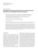
Figure 1 depicts the traffic load during the day for a cluster
of seven neighboring cells. It is worthwhile noticing its typ-
ical “M” shape [14, 15]. That is, during the night there is a
very low traffic load, while during the morning and the af-
ternoon traffic load increases. Besides, two spikes are present
in correspondence of the busiest hours related to business
and commercial activities. In Figure 1, these two spikes are at

12:00 and 19:00, respectively.
2420161284
(Hours)
0
20
40
60
80
100
120
Tr affic in the cluster of cells [Erlang]
Busy hours
Figure 1: Daily traffic in a cluster of 7 neighboring cells.
To identify the size of the time window that satisfies the
stationarity hypothesis for the traffic entering in the cell, we
used the run and the reverse arrangement tests [16] which are
hypothesis tests. They check for the presence of underlying
trends or other variations in random data sequences.
To perform these stationarity tests, it has been assumed
that the interarrival time between calls (i.e., the time between
two successive call requests) is a random process
{T
i
}
n
i
=1
,
where n is the total number of calls during one day. The sta-
tionarity of

{T
i
}
n
i
=1
can be tested by the following steps.
(1) The trace of interarrival times {T
i
}
n
i
=1
is divided into m
subtraces with equal time length (for simplicity mul-
tiples of one hour) obtaining m sequences
{T
(m)
j
}
N
m
j=1
,
where N
m
is the number of samples of the mth sub-
trace.
(2) The mean value for each time interval is computed.
The presence of underlying trends or variations in the

sequence
{T
(m)
j
}
N
m
j=1
is tested, using both the run test
and the reverse arrangement test.
(3) If in a subtrace there is an underlying trend on the
considered time scale (i.e., the considered value of m),
then the subtrace is not stationary with respect to the
mean value.
(4) The size of the time window is decreased (i.e., the
number, m, of subtraces is increased), repeating all the
previous steps until obtaining positive response from
both the tests, for all the subtraces.
We found that in all the cases, with a significance level of 0.05,
data traces pass both the tests only when the size of the time
window does not exceed four hours. Thus, we can analyze the
traffic entering in the cell (and then the call arrival process)
considering only a time window equal to or smaller than four
hours. Given that the uncertainty of any statistical estima-
tion decreases as the sample size increases (i.e., with larger
sample, the influence of outliers is reduced), we chose an in-
terval of four hours (i.e., the maximum window size which
ensures stationarity) around the busiest day hour (i.e., the
time interval with the maximum number of data samples).
4 EURASIP Journal on Wireless Communications and Networking

T = t
r
+ t
c
T
r
= t
r
T
c
= t
c
Answer time
Signaling
complete
time
Ringing
phase
Conversation duration
Call duration
T
c
: Conversation duration
T
r
: Ringing duration
Charging
end time
Time
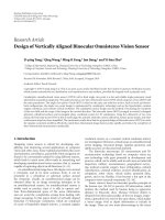
Figure 2: Time diagram to describe call behavior.

In Figure 1 the four hours around the busiest day hour are
highlighted.
Concerning call duration, following a similar procedure
(i.e., using run test and reverse arrangement tests), the sta-
tionarity was verified for any size of the time window. Specifi-
cally, we found that the mean call duration (evaluated in each
hour) does not change appreciably during the day. Therefore,
if we refer to the four hours around the busiest day hour, call
duration is anyway a stationary process.
Given the aforesaid observations, unless otherwise speci-
fied, in the following the analysis will be referred to the four-
hour time window around the busiest hour.
3. DATA ANALYSIS AND CHARACTERIZATION
To characterize the call dropping, we have analyzed the call
arrival process and, specifically, the interarrival time between
two successive new calls. Moreover, the interdeparture time
between two successive dropped calls has been studied (i.e.,
the interval between call dropping instants); in the following,
this time will be simply referred to as interdeparture time.
Likewise, to statistically characterize call duration, we
have analyzed the durations of normally terminated calls
(i.e., not-dropped-calls in operator database) and of dropped
calls, distinguishing two phases: ringing and conversation
(see Figure 2). The duration of the ringing phase is calculated
as the difference between the answer time (i.e., the instant
when the callee answers) and the signaling complete time (i.e.,
the instant when the communication setup finishes). The
conversation duration is the difference between the charging-
end time (i.e., the instant when the billing account stops) and
the answer time. In our analysis, the setup time is not included

in the evaluation of call duration because it does not depend
on user behavior, but only on network characteristics.
The estimation of the mean, μ, and the variance, σ
2
,of
conversation duration (for both dropped and normally ter-
minated calls) and of interarrival and interdeparture times
were carried out. We used the following well-known conver-
gent and not-polarized estimators [13]:
μ =

n
i
=1
x
i
n
,
σ
2
=

n
i
=1

x
i
− μ


2
(n −1)
,(1)
where (x
1
, x
2
, , x
n
) is a sample vector of n elements.
Furthermore, the coefficient of variation, C,definedas
the ratio between standard deviation and mean has been
evaluated; this parameter is an index of data dispersion
around the mean value. In Table 2 , estimated statistical pa-
rameters (referred to 4 hours around the busy hour) are re-
ported for five cells and two clusters of cells.
We observed that the conversation durations of normally
terminated calls and dropped calls show a value of C greater
than 1, whereas the interarrival and the interdeparture times
have a coefficient of variation C
 1. This behavior holds
for both cells and cluster of cells. These results can suggest
the choice of the pdf (probability density function) to rep-
resent each considered process. In particular, we made the
hypothesis, validate by the following statistical analysis, that
conversation duration of normally terminated calls and con-
versation duration of dropped calls have lognormal pdfs with
different parameters [13]:
f
T

(t) =
1
ϕ
√
2πt
e
−(ln t−ϑ)
2
/2ϕ
2
, ϕ, θ>0, t ≥ 0. (2)
It is worthwhile to note that this result extends and gener-
alizes the one reported in [17], where a lognormal function
is used to fit only the channel-holding time in a single cell.
Instead, the conversation duration, considered in this paper,
is the sum of the channel-holding times in all the cells visited
by the user during the same call.
For interarrival and interdeparture times we made the
hypotheses of exponential pdfs, which are density functions
with a coefficient of variation equal to one:
f
X
(t) = λe
−λt
, λ>0, t ≥ 0. (3)
It seems appropriate to mention that, although analysis
of interarrival times has been reported in a previous scientific
paper [17], the study of interdeparture time is a new result of
this paper.
In the next sessions, the previous hypotheses about

pdfs of conversation durations, interarrival time, and inter-
departure time will be verified exploiting two suitable statis-
tical methods.
3.1. Analysis with probability plots
In order to asses if a data set follows a given distribution,
there are some useful graphical tools such as the probability
plot [18].
The idea is to plot, together on the same graph, the cu-
mulative distribution functions of the data sample and of a
specific theoretical distribution, for the same quantile values.
That is, on the axes there are the ordered values of the consid-
ered dataset and the theoretical distribution percentiles. For
a given point on the probability plot, the quantile level is the
same for both the variables on the axes. If the considered dis-
tribution really fits data, the points should lie approximately
on a straight line.
Probability plots can be generated for several competing
distributions to find which provides the best fit. Many aspects
about distribution can be simultaneously tested and detected
Gennaro Boggia et al. 5
Table 2: Estimated statistical parameters.
Number of calls μ[s] σ [s] C
Cell 1
Conversation duration of normally terminated Calls
2339
121.74 205.65 1.69
Conversation duration of dropped calls 96.01 172.09 1.79
Interdeparture time 92.44 87.67 0.95
Interarrival time 6.14 6.14 1.00
Cell 2

Conversation duration of normally terminated calls
2180
93.20 152.18 1.63
Conversation duration of dropped calls 130.20 339.70 2.61
Interdeparture time 67.72 78.23 1.16
Interarrival time 6.60 6.54 0.99
Cell 3
Conversation duration of normally terminated calls
4555
100.97 134.89 1.34
Conversation duration of dropped calls 92.86 159.35 1.72
Interdeparture time 101.08 103.33 1.02
Interarrival time 3.18 3.53 1.11
Cell 4
Conversation duration of normally terminated calls
2200
111.15 187.50 1.69
Conversation duration of dropped calls 95.64 213.47 2.23
Interdeparture time 85.01 94.28 1.11
Interarrival time 6.54 7.01 1.07
Cell 5
Conversation duration of normally terminated calls
3586
108.35 198.13 1.83
Conversation duration of dropped calls 97.27 174.25 1.79
Interdeparture time 99.65 101.27 1.01
Interarrival time 4.00 5.00 1.25
Cluster 1
Conversation duration of normally terminated calls
11748

100.41 212.21 2.10
Conversation duration of dropped calls 94.92 199.69 2.11
Interdeparture time 27.25 27.23 0.99
Interarrival time 1.25 1.41 1.13
Cluster 2
Conversation duration of normally terminated calls
4448
107.70 208.94 1.94
Conversation duration of dropped calls 91.42 161.67 1.77
Interdeparture time 74.48 79.34 1.07
Interarrival time 3.47 13.23 1.05
from this plot: shifts in location, shifts in scale, changes in
symmetry, and the presence of outliers (see for details [18]).
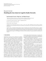
To verify our hypothesis about pdf of the conversation
time, we can consider the probability plot for the logarithm
of conversation duration versus the normal standard distri-
bution. In fact, as well known, the normal and lognormal
distributions are closely related, that is, if X is lognormally
distributed with parameters θ and ϕ, then log (X)isnormally
distributed with the same parameters [13]. For example, with
reference to the normally terminated calls in a cell monitored
for 4 hours, Figure 3 reports the probability plot for the log-
arithm of conversation duration versus normal standard dis-
tribution. A similar result holds also for the conversation du-
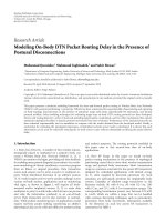
ration of dropped calls. Figure 4 shows the probability plot
for the interarrival time versus the exponential distribution.
From both figures, it can be noticed that data lie
on a straight line, confirming our hypotheses about pdfs.
We highlight that also the probability plots for the inter-
departure time between dropped calls, which have not been

reported for lack of space, show similar agreement.
Regarding the ringing time, T
r
, measures have shown
that there are many values close to zero, a lot of values around
5 seconds, and few larger values. So that, it does not follow
any known distribution. By using again the probability plots
(not reported for lack of space), it has been verified that a
suitable pdf for fitting ringing time data was a weighted mix-
ture of exponential and lognormal pdfs:
f
T
r
(t) = αλe
−λt
+
(1
−α)
ϕ
√
2πt
e
−(1/2)((log (t)−θ)/ϕ)
2
; t ≥ 0, α ∈ [0, 1],
(4)
where α is a weight coefficient.
3.2. The χ
2
-goodness-of-fit-test results

The probability plot remains a qualitative graphical test. To
confirm our assumption, we need to deploy also a hypothesis
test such as the χ
2
-goodness-of-fit test (χ
2
-test) [19]. Such a
test requires the estimation, from the sample data, of param-
eters for each distribution under testing.
We use the well-known maximum likelihood method
[13]. Let X be a random variable with its pdf dependent on
the parameter γ and let
f (X, γ)
= f

x
1
, γ

·f

x
2
, γ

···f

x
n
, γ


(5)
6 EURASIP Journal on Wireless Communications and Networking
43210−1−2−3−4
Standard normal percentiles
0
1
2
3
4
5
6
7
8
9
Log. of conversation duration percentiles
Data sample
Lognormal distribution
Figure 3: Probability plot for the logarithm of conversation dura-
tion (for normally terminated calls) versus normal standard distri-
bution.
454035302520151050
Exponential percentiles
0
5
10
15
20
25
30

35
40
45
Percentiles of call interarrival time (s)
Data sample
Exponential distribution
Figure 4: Probability plot of calls interarrival time versus exponen-
tial distribution.
be the joint density function of n samples x
i
of X. This den-
sity, considered as a function of γ, is called the likelihood func-
tion of X.
The value γ
∗
of γ that maximizes f (X, γ) is the maxi-
mum likelihood estimation of γ. The logarithm of f (X, γ),
L(X, γ)
= ln f (X, γ) =
n

i=l
ln f

x
i
, γ

,(6)
is the log-likelihood function of X.

From the monotonicity of logarithm, it follows that γ
∗
also maximizes the function L(x,γ) and is the solution of the
equation
∂L(X, γ)
∂γ
=
n

i=1
1
f

x
i
, γ

∂f

x
i
, γ

∂γ
= 0. (7)
As shown in [13], the maximum likelihood estimator is
asymptotically normal, unbiased, with minimum variance.
For our purpose, the maximum likelihood estimators for
the parameters of the exponential and the lognormal pdfs
can be easily obtained solving (7) applied to (2)and(3). The

estimators are, respectively (see [13, 17]),

λ = n/
n

i=1
t
i
,

ϑ =
1
n
n

i=1
ln

t
i

, ϕ =
1
n
n

i=1
ln

t

i

2
−

ϑ
2
,
(8)
where t
i
are the time samples.
Unfortunately, it is not possible to obtain a closed form
expression for the four estimators of the parameters in (4),
since from (7) we obtain a nonlinear equation system. Nev-
ertheless, such a system can be solved by numerical methods.
Specifically, as described in [20, 21], a subspace trust region
method based on the interior-reflective Newton method has
been implemented.
Now, we can apply the χ
2
-test to check our hypothe-
ses about pdfs following the algorithm introduced by Fisher
[19]. Using the significance level α
= 0.01, the tests gave pos-
itive results in all the trials. As in [17], also in this work it was
necessary to filter data samples which showed an anomalous
relative frequency. But, whereas in [17] the 26% of the sam-
ple data were rejected, in our analysis never more than 5% of
data have been discharged.

The obtained results show that both conversation dura-
tions of normally terminated calls and dropped calls are log-
normal distributed. Moreover, our statistical analysis con-
firms the exponential hypothesis both for interarrival time
between two successive new calls and for the interdeparture
time between two successive dropped calls. Finally, χ
2
-test
confirms that ringing time has the pdf reported in (4). Even
if some of this results are similar to previous ones [17], we
highlight that, to the best of our knowledge, the analyses of
interdeparture time, of conversation duration for dropped
calls, and of ringing time do not appear in any previous sci-
entific papers.
As an example, in Figure 5 the measured data and the fit-
ted lognormal pdf for the conversation duration of normal
terminated calls are reported. In Figure 6, the same informa-
tion is reported, but referring to the dropped calls. In Figures
7 and 8 the interdeparture time between dropped calls and
the interarrival time between calls are fitted by exponential
pdfs. Finally, in Figure 9 the ringing duration pdf of a clus-
ter of 7 cells monitored for 4 hours is fitted by a mixture of
exponential and lognormal pdfs. We point out that the con-
clusions about the characterization of call durations, inter-
arrival time between calls, and interdeparture time between
dropped calls hold both for single cells and for cell clusters.
4. ANALYTICAL MODEL
In this section, starting from the results of data analysis, a
new analytical model to predict the drop-call probability as a
function of traffic parameters has been developed.

As verified in the previous section, the interarrival times
for new calls and interdeparture time for dropped calls have
an exponential distribution. With the additional hypotheses
Gennaro Boggia et al. 7
350300250200150100500
Conversation duration (s)
0
5
10
15
20
25
30
35
40
Number of calls
Samples
Lognormal fitting
Figure 5: Fitting of conversation duration of normally terminated
calls with a lognormal pdf (cell 1 observed for 4 hours).
300250200150100500
Conversation duration (s)
0
2
4
6
8
10
12
Number of dropped calls

Samples
Lognormal fitting
Figure 6: Fitting of conversation duration of dropped calls with a
lognormal pdf (cell 1 observed for 4 hours).
of independence for both arrival events and dropping events,
we can state that these processes can be considered Poisso-
nian. This result extends the one reported in [14] in which,
starting from measures, the classical Poisson hypothesis is
verified only for call arrivals.
In this way, we can model all the causes of call dropping
as a single phenomenon which follows the Poisson statistic.
Let λ
t
be the total traffic entering in the generic cell. Since
in a well-established cellular network the call-blocking prob-
ability is almost negligible (i.e., the system can be considered
as nonblocking), λ
t
is also the total traffic accepted in the cell.
5004003002001000
Interdeparture time between dropped calls (s)
0
1
2
3
4
5
6
7
8

9
10
Number of samples
Samples
Exponential fitting
Figure 7: Fitting of interdeparture time between dropped calls with
an exponential pdf (cell 1 observed for 24 hours).
302520151050
Interarrival time between calls (s)
0
50
100
150
200
250
300
Number of samples
Samples
Exponential fitting
Figure 8: Fitting of interarrival time between calls with an expo-
nential pdf (cell 1 observed for 4 hours).
The drop call probability, P
d
, is equal to the fraction of this
traffic dropped due to the phenomena described in Section 2.
To e v a l u a t e P
d
, let us consider, for sake of simplicity, the
probability that a call is normally terminated, P
nt

, related to
P
d
by the following expression:
P
d
= 1 −P
nt
. (9)
A call request is served by a generic channel, randomly
selected, and the call will finish, if correctly terminated, after
a duration time, T (see Figure 2). From the results reported
8 EURASIP Journal on Wireless Communications and Networking
50403020100
Ring duration (s)
0
200
400
600
800
1000
1200
1400
Number of calls
Samples
Fitting
Figure 9: Fitting of ringing duration with a mix of exponential and
lognormal pdf (cluster 1 observed for 4 hours).
in the previous section, we can state that the call duration,
T, is the sum of the two random variables T

r
and T
c
which
model the ringing and conversation times, respectively. The
random variable (r.v.) T
r
models the ringing duration with
a pdf f
T
r
(t), according to (4). The r.v. T
c
models the con-
versation duration with a lognormal pdf f
T
c
(t), according to
(2). Assuming that T
r
and T
c
are independent, the pdf f
T
(t)
of the call duration for the normally terminated calls can be
obtained as the following convolution between pdfs [13]:
f
T
(t) = f

T
r
(t)∗f
T
c
(t) =

t
0
f
T
c
(t −τ)·f
T
r
(τ)dτ. (10)
The probability P
nd
(1) that a call, among k active ones, is
not involved by a single drop event (i.e., call is not dropped),
during the duration time T
= t,is(k−1)/k.Obviously,given
that drop events are assumed to be independent, if there are
n drop events, this probability becomes
P
nd
(n) =

k −1
k


n
. (11)
On the other hand, as said before, dropping events con-
stitute a Poisson process; let ν
d
be its intensity. Hence, if Y
is the r.v. which counts the number of drops, the probability
that there are n drops in the interval T
= t is [13]
P(Y
= n) =

ν
d
t

n
n!
e
−ν
d
t
, n ≥ 0. (12)
By using (11)and(12), the probability that a call with
duration T
= t is normally terminated, in the presence of k
contemporary calls and n drop events, is equal to the proba-
bility that drop events do not affect the considered call:
P

nt
(T = t,k, n) = P
nd
(n)·P(Y = n) =

k −1
k

n

ν
d
t

n
n!
e
−ν
d
t
.
(13)
By applying the total probability theorem to the number
of drop events, the probability that a call with duration T
= t
is normally terminated, in the presence of k contemporary
calls (i.e., the call is not dropped), can be estimated as
P
nt
(T = t,k) =

∞

n=0
P
nt
(T = t,k, n)
=
∞

n=0

k −1
k

n

ν
d
t

n
n!
e
−ν
d
t
= e
−ν
d
t

∞

n=0
1
n!

(k −1)ν
d
t
k

n
= e
−ν
d
t
·e
((k−1)/k) ν
d
t
= e
−ν
d
t/k
.
(14)
Using again the total probability theorem, summing over
all the possible numbers of contemporary active calls, the
probability that a call is normally terminated with duration t
is

P
nt
(T = t) =
∞

k=1
P
nt
(T = t,k)·P
a
(k), (15)
where P
a
(k) is the probability that there are k active users
(i.e., k calls in progress).
As experimentally verified (see Section 2), in well-
established cellular networks operating in normal condi-
tions, the call dropping is not due to unavailability of com-
munication channels (i.e., the blocking and handover prob-
abilities are negligible). Thus, we can model the system as a
queue with infinite number of servers, which is a nonblock-
ing queue. Considering as service time the call duration, we
have to consider a queue with a general service time distribu-
tion. This means that, by using the queuing theory notation
[22], the system can be modeled as an M/G/
∞ queue. There-
fore, the probability P
a
(k) that there are k active users is given
by [22]

P
a
(k) = c
N
·
ρ
k
k!
, k
≥ 1, (16)
where ρ is the utilization factor, given by the product between
the total traffic λ
t
and the mean service time E[T]; c
N
is a nor-
malization coefficient which considers that there is at least
one ongoing call.
Applying the normalization condition, the coefficient c
N
is evaluated as
c
N
=
1
e
ρ
−1
. (17)
Note that exploiting the utilization factor ρ, we can also

evaluate the mean number of active users E[N]:
E[N]
=
∞

k=1
k·c
N
ρ
k
k!
=
e
ρ
e
ρ
−1
ρ. (18)
Using (17)in(16), we obtain
P
a
(k) =
1
e
ρ
−1
·
ρ
k
k!

, k
≥ 1. (19)
Gennaro Boggia et al. 9
Substituting (19)and(14)in(15), we have
P
nt
(T = t) =
∞

k=1
e
−ν
d
t/k
·
1
e
ρ
−1
·
ρ
k
k!
. (20)
Now, it is straightforward to evaluate the probability of a
normally terminated call, P
nt
, simply considering every pos-
sible call duration:
P

nt
=

∞
0
P
nt
(T = t) f
T
(t)dt
=
1
e
ρ
−1
∞

k=1
ρ
k
k!

∞
0
f
T
(t)e
−ν
d
t/k

dt,
(21)
where f
T
(t) is the pdf defined by (10).
Finally, from (9), it results that the drop-call probability
is
P
d
= 1 −
1
e
ρ
−1
∞

k=1
ρ
k
k!

∞
0
f
T
(t)e
−ν
d
t/k
dt. (22)

It is worth noticing that (22) depends on the drop-call
rate ν
d
, the pdf f
T
(t) of the call duration of normally termi-
nated calls, and the utilization factor ρ (which in turn de-
pends on the traffic λ
t
).
Equation (22) can be exploited to study the effect of traf-
fic parameters on drop-call probability, but it can be also ap-
plied to predict such a probability starting from real data.
In the latter case, equation parameters should be obtained
from measured data following the same analysis described in
Section 3.
The development of our model did not require any as-
sumption on a particular technology. Thus, the model can
be exploited to predict the drop-call probability in different
cellular networks (e.g., PCS, UMTS). In fact, we need only
measured datasets to find the pdfs that best fit ringing time,
conversation duration, interarrival time, and interdeparture
time. Then, we can characterize (10) and find the drop-call
probability in this kind of systems by applying (22).
5. NUMERICAL RESULTS
The developed model has been validated by using the real
data analyzed in Section 3. Moreover, it has been exploited
to study the effect of its parameter on network performance
(i.e., we evaluated the model sensitivity to its parameters).
For the validation, in each considered cell, the drop-call

probability and its confidence interval [13] (with confidence
level 1
− α = 0.95) have been estimated directly from mea-
sured data. This is to establish the acceptance region for re-
sults from our model. Then, the drop call probability has
been analytically estimated just applying (22). Parameters of
this equation have been obtained by the data analysis re-
ported in Section 3. Results coming out from the analytical
model can be considered acceptable if they fall in the confi-
dence interval of the measured drop-call probability.
In Ta ble 3 , results of validation are reported for the
same cells and cluster of cells considered in Tabl e 2 (i.e., the
datasets for which we have explicitly reported numerical re-
sults of statistical analysis). They show that, in every case, the
Table 3: Drop-call probability results.
(By measures) (By model) Confidence interval
P
d
[%] P
d
[%] [%]
Cell 1 6.79 6.52 [5.84; 7.88]
Cell 2 7.29 7.47 [6.27; 8.46]
Cell 3 3.07 3.12 [2.61; 3.61]
Cell 4 6.72 6.74 [5.75; 7.84]
Cell 5 4.04 4.00 [3.44; 4.74]
Cluster 1 4.61 4.29 [4.13; 5.14]
Cluster 2 4.68 4.34 [4.08; 5.37]
0.140.120.10.08
λ

t
(call/h)
0
0.005
0.01
0.015
0.02
0.025
0.03
ν
d
-drop-call rate
Samples of ν
d
vs. λ
t
Least mean square linear fitting
Figure 10: Total entering trafficinacell,λ
t
, versus the drop-call
rate, ν
d
.
analytical results fall in the confidence interval of measured
drop-call probability. This result has been confirmed for all
the sets of measured data, thus validating our model.
A better agreement between real data and model results
could be achieved by using larger data sample [13]. In fact,
as the dataset gets larger, the confidence interval gets smaller.
Hence, the estimation of the input parameters (i.e., ν

d
, λ
t
,
and so on) for the analytical model gets more accurate. It
is evident from the comparison of Tables 2 and 3 that the
narrowest confidence intervals (i.e., the better estimations for
our model) correspond to the largest datasets (i.e., Cell 3 and
Cluster 1).
Themodelcanbealsoexploitedtoevaluatenetworkper-
formance as a function of traffic parameters. For example, it
allows us to asses the sensitivity of the drop call probability
to call duration distribution, to the offered trafficload,and
so on. To this aim, first the correlation between ν
d
and λ
t
has
been studied from data. We found that a linear dependence
between these two parameters exists, that is,
ν
d
= mλ
t
+ b, (23)
where m and b could be obtained with a least square regres-
sion technique [13].
Figure 10 shows that relatively large variations of λ
t
pro-

duce only small changes for ν
d
.
10 EURASIP Journal on Wireless Communications and Networking
0.40.350.30.250.20.150.1
λ
t
(call/s)
0.02
0.03
0.04
0.05
0.06
0.07
0.08
0.09
0.1
P
d
-drop-call probability
E[T
c
] = 70 s
E[T
c
] = 100 s
E[T
c
] = 130 s
Figure 11: Drop-call probability versus traffic λ

t
with several mean
conversation durations.
Hence, in (22) the effect of the drop call rate ν
d
can be
studied by considering only the effect of the call arrival rate
λ
t
. At the same time, the other parameter of the model (i.e.,
the utilization factor ρ) is defined as the product between the
mean call duration E[T] and the call arrival rate λ
t
. There-
fore, we can simply analyze the impact on model results of
the call-arrival rate and of the call duration.
In Figure 11, the drop-call probability obtained by the
model is reported as a function of the total traffic entering
in the cell, λ
t
(measured in calls per second [call/s]). The
graphs are reported for several values of the mean conversa-
tion duration E[T
c
] (from 70 seconds to 130 seconds) with a
fixed coefficient of variation, C, equal to 1.3, near to the typi-
cal value observed in measured data (see Ta bl e 2 ). The mean
ringing duration is equal to 10 seconds. The drop call rate ν
d
was varied accordingly with (23).

System performance improves as the traffic entering in
the cell increases. Since there is a linear dependence between
λ
t
and ν
d
, increasing the traffic load, the number of dropped
calls remains quite constant. For this reason, the drop-call
rate decreases.
Furthermore, drop-call probability remains quite con-
stant when mean call duration increases. Only for small val-
ues of λ
t
, that is, for a low traffic load, there are appreciable
differences.
In Figure 12, the drop-call probability is reported as a
function of the total traffic entering in the cell, λ
t
,withsev-
eral values for the coefficient of variation. The mean con-
versation duration is assumed equal to 100 seconds, near to
the typical value observed in the measured data (see Table 2 ).
The other system parameters have the same values used for
obtaining Figure 11.
The more interesting result coming out from this figure
is the effect of coefficient of variation on drop-call proba-
bility, particularly at low traffic load. This probability de-
creasesascoefficient of variation increases; that is, fixing
mean conversation duration, values more dispersed around
this mean reduce drop-call probability. Similar results on

0.40.350.30.250.20.150.1
λ
t
(call/s)
0.02
0.03
0.04
0.05
0.06
0.07
0.08
0.09
0.1
P
d
-drop-call probability
Coefficients of variation C = 1.8
Coefficients of variation C
= 2.1
Coefficients of variation C
= 2.4
Figure 12: Drop-call probability versus traffic λ
t
with several coef-
ficients of variation C.
0.40.350.30.250.20.150.1
λ
t
(call/s)
0

0.02
0.04
0.06
0.08
0.1
P
d
-drop-call probability
E[T
r
] = 6s
E[T
r
] = 10 s
E[T
r
] = 14 s
Figure 13: Drop-call probability versus λ
T
with several mean ring-
ing durations.
other system performance parameters are reported in liter-
ature [2, 23]. Such a behavior can partially explain the per-
formance improvement of some well-established mobile net-
works. In fact, in these networks the presence at the same
time of many different services leads to a larger differenti-
ation of call durations; consequently, values are more dis-
persed around the mean and the drop-call probability gets
smaller.
Finally, Figure 13 reports the sensitivity of the pro-

posed model as a function of λ
T
, for several values of the
mean ringing duration. The mean call duration is equal to
100 seconds. The other model parameters are the same previ-
ously used. It is worth noting that ringing duration variation
does not affect the drop-call probability. In fact, the curves
for the different E[T
r
] values are practically indistinguish-
able.
Gennaro Boggia et al. 11
6. CONCLUSIONS
In this paper, starting from the statistical analysis of data
measured in a large real well-established cellular network, a
new model to study the call-dropping phenomenon has been
developed.
We started from the verification that handover failure,
considered prevailing in the classical cellular performance
models, has become negligible in this kind of networks. With
both planning optimization and fine tuning of network pa-
rameters, several secondary phenomena (e.g., irregular user
behaviors, abnormal network response, power attenuation,
and so on) become significant. This requires new modeling
of the call dropping process.
Using statistical tools on measured data from a real net-
work, we have characterized dropped calls and call durations
(distinguishing between ringing and conversation phases).
Results of this data analysis have driven the development of
a new analytical model which relates drop-call probability to

the drop-call rate, the pdf of the call duration, and the traffic
load.
The proposed model has been validated comparing its re-
sults with the ones obtained by measures, in a wide range of
traffic load conditions for both cells and cluster of neighbor-
ing cells. Moreover, the impact of its parameters on drop-call
probability has been studied.
The developed model can be easily extended to differ-
ent cellular networks simply characterizing the distribution
of the call duration.
ACKNOWLEDGMENTS
The authors would like to thank Dr. Massimo Siviero from
Vodafone, Italy, for his helpful contribution in this work; in
particular, in the phase of measure collection. A preliminary
version of this paper was presented at IEEE VTC’05 Spring
Conference.
REFERENCES
[1] D. Hong and S. Rappaport, “Traffic model and performance
analysis for cellular mobile radio telephone systems with pri-
oritized and nonprioritized handoff procedures,” IEEE Trans-
actions on Vehicular Technology, vol. 35, no. 3, pp. 77–92, 1986.
[2] P.V.OrlikandS.S.Rappaport,“Amodelforteletrafficperfor-
mance and channel holding time characterization in wireless
cellular communication with general session and dwell time
distributions,” IEEE Journal on Selected Areas in Communica-
tions, vol. 16, no. 5, pp. 788–803, 1998.
[3] H. Zeng, Y. Fang, and I. Chlamtac, “Call blocking performance
study for PCS networks under more realistic mobility assump-
tions,” Telecommunication Systems, vol. 19, no. 2, pp. 125–146,
2002.

[4] Y. Fang, I. Chlamtac, and Y B. Lin, “Call performance for a
PCS network,” IEEE Journal on Selected Areas in Communica-
tions, vol. 15, no. 8, pp. 1568–1581, 1997.
[5] Y. Fang, I. Chlamtac, and Y B. Lin, “Modeling PCS networks
under general call holding time and cell residence time distri-
butions,” IEEE/ACM Transactions on Networking, vol. 5, no. 6,
pp. 893–906, 1997.
[6] Y. Fang and I. Chlamtac, “Teletraffic analysis and mobility
modeling of PCS networks,” IEEE Transactions on Communi-
cations, vol. 47, no. 7, pp. 1062–1072, 1999.
[7] M. Rajaratnam and F. Takawira, “Nonclassical trafficmodel-
ing and performance analysis of cellular mobile networks with
and without channel reservation,” IEEE Transactions on Vehic-
ular Technology, vol. 49, no. 3, pp. 817–834, 2000.
[8] M. Rajaratnam and F. Takawira, “Handoff traffic characteriza-
tion in cellular networks under nonclassical arrivals and ser-
vice time distributions,” IEEE Transactions on Vehicular Tech-
nology, vol. 50, no. 4, pp. 954–970, 2001.
[9] Y. Iraqi and R. Boutaba, “Handoff and call dropping probabil-
ities in wireless cellular networks,” in Proceedings of Interna-
tional Conference on Wireless Networks, Communications and
Mobile Computing (WIRELESSCOM ’05), vol. 1, pp. 209–213,
Maui, Hawaii, USA, June 2005.
[10] X. Chao and W. Li, “Performance analysis of a cellular network
with multiple classes of calls,” IEEE Transactions on Communi-
cations, vol. 53, no. 9, pp. 1542–1550, 2005.
[11] N. Nasser, “Enhanced blocking probability in adaptive multi-
media wireless networks,” in Proceedings of the 25th IEEE Inter-
national Performance, Computing, and Communications Con-
ference (IPCCC ’06), vol. 2006, pp. 647–652, New Orleans, La,

USA, April 2006.
[12] G. Boggia, P. Camarda, and N. Di Fonzo, “Teletraffic analysis
of hierarchical cellular communication networks,” IEEE Trans-
actions on Vehicular Technology, vol. 52, no. 4, pp. 931–946,
2003.
[13] A. Papoulis, Probability, Random Variables and Stochastic Pro-
cesses, McGraw-Hill, New York, NY, USA, 3rd edition, 1991.
[14] S. Bregni, R. Cioffi, and M. Decina, “WLC09-1: an empiri-
cal study on statistical properties of GSM telephone call ar-
rivals,” in Proceedings of IEEE Global Telecommunications Con-
ference (GLOBECOM ’06), pp. 1–5, San Francisco, Calif, USA,
November-December 2006.
[15] A. Pattavina and A. Parini, “Modelling voice call interarrival
and holding time distributions in mobile network,” in Pro-
ceedings of the 19th International Te letraffic Congress (ITC ’05),
Beijing, China, August 2005.
[16] J. S. Bendat and A. G. Piersol, Random Data, Analysis and Mea-
surement Procedures, John Wiley & Sons, New York, NY, USA,
2nd edition, 1986.
[17] C. Jedrzycki and V. M. Leung, “Probability distribution
of channel holding time in cellular telephony systems,” in
Proceedings of IEEE 46th Vehicular Technology Conference
(VTC ’96), vol. 1, pp. 247–251, Atlanta, Ga, USA, May 1996.
[18] J. M Chambers, W. S. Cleveland, B. Kleiner, and P. A.
Tuke y, Graphical Methods for Data Analysis, Chapman & Hall,
Boston, Mass, USA, 1983.
[19] E. Kreyszig, Advanced Engineering Mathematics, John Wiley &
Sons, New York, NY, USA, 6th edition, 1987.
[20] T. F. Coleman and Y. Li, “On the convergence of interior-
reflective Newton methods for nonlinear minimization sub-

ject to bounds,” Mathematical Programming, vol. 67, no. 1–3,
pp. 189–224, 1994.
[21] T. F. Coleman and Y. Li, “An interior trust region approach for
nonlinear minimization subject to bounds,” SIAM Journal on
Optimization, vol. 6, no. 2, pp. 418–445, 1996.
[22] L. Kleinrock, Queuing Systems: Computer Applications, vol. 2,
John Wiley & Sons, New York, NY, USA, 1985.
[23] F. Khan and D. Zeghlache, “Effect of cell residence time dis-
tribution on the performance of cellular mobile networks,” in
Proceedings of the IEEE 47th Vehicular Technology Conference
(VTC ’97), vol. 2, pp. 949–953, Phoenix, Ariz, USA, May 1997.