Báo cáo hóa học: " Research Article Temperature-Aware Routing for Telemedicine Applications in Embedded Biomedical Sensor Networks" ppt

Hindawi Publishing Corporation
EURASIP Journal on Wireless Communications and Networking
Volume 2008, Article ID 572636, 11 pages
doi:10.1155/2008/572636
Research Article
Temperature-Aware Routing for Telemedicine Applications in
Embedded Biomedical Sensor Networks
Daisuke Takahashi,
1
Yang Xiao,
1
Fei Hu,
2
Jiming Chen,
3
and Youxian Sun
3
1
Department of Computer Science, The University of Alabama, Tuscaloosa, AL 35487, USA
2
Computer Engineering Depar tment, Rochester Institute of Te chnology, Rochester, NY 14623, USA
3
State Key Laboratory of Industrial Control Technology, Institute of Industrial Process Control, Zhejiang University,
Hangzhou 310027, China
Correspondence should be addressed to Yang Xiao,
Received 13 April 2007; Revised 3 November 2007; Accepted 2 December 2007
Recommended by Hui Chen
Biomedical sensors, called invivo sensors, are implanted in human bodies, and cause some harmful effects on surrounding body
tissues. Particularly, temperature rise of the invivo sensors is dangerous for surrounding tissues, and a high temperature may
damage them from a long term monitoring. In this paper, we propose a thermal-aware routing algorithm, called least total-route-
temperature (LTRT) protocol, in which nodes temperatures are converted into graph weights, and minimum temperature routes

are obtained. Furthermore, we provide an extensive simulation evaluation for comparing several other related schemes. Simulation
results show the advantages of the proposed scheme.
Copyright © 2008 Daisuke Takahashi et al. This is an open access article distributed under the Creative Commons Attribution
License, which permits unrestricted use, distribution, and reproduction in any medium, provided the original work is properly
cited.
1. INTRODUCTION
Telemedicine enables doctors to carry out remote diagnoses
far from the patients. There are many researches on mobile
telemedicine, for example, [1–23]. Telemedicine can be de-
fined as an information technology that enables doctors to
perform medical consultations or diagnoses away from pa-
tients. In other words, doctors can remotely examine patients
by viewing and asking symptoms via monitors and sound de-
vices, and gathering physiological data through the telecom-
munication, with which another end is set up at the patients
sites.
One application of telemedicine using wearable wireless
body area network architecture aims to implant biomedical
sensors in human bodies. This kind of biomedical sensors is
called invivo sensors. Like basic wearable vital sensors, the
invivo sensors can sample a variety of biometric data, and
transmit them to practitioners terminals, such as PDAs or
tablet PCs, using the shortrange wireless connectivity [1–
5, 19]. Furthermore, communications between the invivo
sensors and the terminals often involve multihop transmis-
sions to avoid entire energy consumption [1]. Currently, the
invivo sensors are applied to an artificial retina, glucose level
monitoring, organ monitoring, and cancer detecting [2].
However, implanting biomedical sensors into human
bodies may cause some harmful effects on surrounding body

tissues. Since the invivo sensors usually transmit or relay
biomedical data to neighboring sensor nodes from time to
time, heat caused by processing and communication will ap-
pear inside of human bodies. Obviously, this temperature
rise of the invivo sensors is dangerous for surrounding tis-
sues, and a high temperature may damage them from a long-
term monitoring [1, 3]. Thus, regarding the invivo sensors,
routing protocols need to be designed to suppress the tem-
perature rise up to a predefined threshold, that is, data trans-
missions among the sensors should disperse around net-
works and not rely on only one route [1]. In addition, for the
sake of reducing exposure of infrared radiation (IR) (a kind
of electromagnetic radiation), consideration of power con-
sumption of batteries is of importance. Because lower bat-
teries require recharging by IR, easily expending battery life
should be required to recharge often, and this increases ex-
posing body tissues to IR and should be avoided [6–9]. Of
course, the latency of the network communication is also
considered for critical situations.
In this paper, we propose a least total-route-temperature
(LTRT) protocol, in which nodes temperatures are converted
into graph weights, and minimum temperature routes are
2 EURASIP Journal on Wireless Communications and Networking
H
H
H
H
S
Sender
1st neighbor node

Hot spot
Destination
D
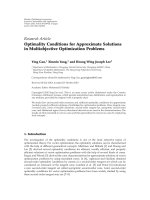
Figure 1: An example of TARA.
obtained. Furthermore, we provide an extensive simulation
evaluation for comparing several other related schemes in-
cluding the proposed scheme.
The rest of the paper is organized as follows. Section 2
provides a survey of thermal-aware routing algorithms. We
propose the LTRT protocol in Section 3. Simulations are
presented in Section 4. Finally, we conclude the paper in
Section 5.
2. THERMAL-AWARE ROUTING ALGORITHMS
To avoid the heat generation, basically, three thermal-aware
routing algorithms were proposed: thermal-aware routing al-
gorithm (TARA), least temperature routing (LTR) protocol,
and adaptive least temperature routing (ALTR) protocol [2].
In this section, we introduce these three thermal-aware rout-
ing algorithms.
2.1. Thermal-aware routing algorithm (TARA)
When biomedical sensors are implanted into human bod-
ies, the temperature rise must be taken into account to
avoid damaging surrounding body tissues. In addition, upon
running out of batteries, the invivo sensors require to be
rechargedbyIRradiation.However,thisIRradiationalso
causes the temperature rise of the sensors. Therefore, the
number of times to recharge sensor batteries is preferably re-
duced by prolonging battery life as long as possible [6–9].
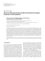
Thermal-aware routing algorithm (TARA), shown in
Figure 1, is designed for solving these constraints [6]. At first,

TARA defines hot spots as areas where sensor nodes have rel-
atively high temperature due to focusing data communica-
tions [6]. Upon detecting the hot spots, not to produce the
temperature rise of these areas any longer, TARA attempts to
establish another route to detour around the hot spots us-
ing a withdrawal strategy [6]. In this strategy, upon receiv-
ing packets, when surrounding (neighboring) nodes—except
for a sending node—are all hot spots, current node will send
back packets to the sender node, and the sender node will
then select an alternative route to detour the hot spots or may
send it back to its previous node, and so on [6]. After cool-
ing a temperature of the hot spots down to a predefined limit,
H
H
H
H
H
S
L
L
L
L
L
L
D
Hot spots
Neighboring nodes that have
the least temperature
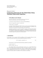
Figure 2: An example of LTR.
TARA takes these nodes into consideration as new candidates

of later routing. To accomplish TARA effectively, every node
must know temperature changes of neighboring nodes by al-
ways monitoring neighbors packet counts, and calculating
communication radiation and power consumption to derive
current temperature of the neighbors. The hot spots, which
exceed a predefined minimum limit of temperature, must be
checked by surrounding sensors, and later avoid participat-
ing in routing until temperature is standardized.
Figure 1 illustrates an example of TARA. A sender first
tries to send packets to a neighboring node (1st neighboring
node) that is on the way to the destination and not a hot
spot. However, this neighboring node is surrounded by hot
spots within its communication range. Therefore, it sends the
packets back to the sender again, and the sender chooses an
alternative node that is not a hot spot. The packets detour the
hot spots to the destination as illustrated in Figure 1.
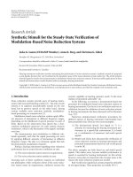
2.2. Least temperature routing (LTR)
Similar to TARA, least temperature routing (LTR) protocol,
shown in Figure 2, is designed to avoid establishing routes on
the hot spots aiming to keep temperature low in particular
invivo sensor nodes [1]. However, unlike TARA, LTR always
chooses neighboring nodes which have the lowest tempera-
ture for its routing [1]. Therefore, unless packets aim to be
sent to a neighboring node which is the destination of the
packets, current nodes always send the packets to the coolest
neighbors and seek for the destination [1]. Besides, LTR also
employs a packet discarding for the sake of maintaining the
network bandwidth [1]. Each packet roaming in a network
maintains its hop count by each hop. Compared with a pre-
defined minimum hop count, namely, MAX

HOPS, if the
value of the hop count exceeds MAX
HOPS, the current sen-
sor node will throw away the packet from the network. In
addition, to avoid infinitely looping the same route, packets
wandering in a network can maintain a table which keeps
track of sensor nodes that the packets have most recently
passed through [1]. Thus, if a next node, where the packets
will be forwarded (the coolest neighbor), is already on the
table, the current node will pass the packets to the second
lowest temperature node which is not on the table to avoid
Daisuke Takahashi et al. 3
H
H
H
H
H
S
L
L
L
L
L
L
D
Hot spots
Neighboring nodes that
have the least temperature
At this point,
a packet exceeds

its predefined
hop count
threshold
Alternative
path by SHR
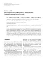
Figure 3: An example of ALTR.
choosing the same route. This consequently avoids infinitely
looping over the same route. Figure 3 illustrates an example
of LTR, which always chooses nodes that have the least tem-
perature.
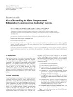
2.3. Adaptive least temperature routing (ALTR)
One variant of LTR protocol is adaptive least tempera-
ture routing (ALTR) protocol. A difference between LTR
and ALTR is that while ALTR as in LTR employs a
packet hop count and keeps track of the hop count of
each packet in every hop, when the value of the hop
count exceeds a predefined minimum hop count, namely,
MAX
HOPS ADAPTIVE, it can use the shortest hop-routing
(SHR) protocol as an alternative protocol to take the packets
to the destination as soon as possible [1]. From the name of
“adaptive” least temperature routing, ALTR can adapt to par-
ticular topologies since in some network topologies, such as
a ring topology, packet sequences inevitably trace the same
path and temperature of sensor nodes on particular paths
and the scheme will get higher rapidly, with a proactive de-
lay mechanism utilized [1]. In this “proactive delay” mech-
anism, upon getting a packet from some neighboring node,
when there are at most two ways to send the packet but their
temperatures are comparatively high, the current node can

wait a unit time for sending it to the coolest neighbor for the
sake of calming down their temperature [1]. Although the
packet latency somewhat becomes higher, the average tem-
perature of networks can get lower [1]. Figure 3 illustrates an
example of ALTR, which basically chooses nodes that have
the least temperature until packets exceed a predefined hop-
count threshold, MAX
HOPS ADAPTIVE. Upon exceeding
the threshold, packets simply choose nodes which can send
them to the destination in the minimum hop count by using
the shortest hop routing (SHR).
3. LEAST TOTAL-ROUTE TEMPERATURE (LTRT)
In this section, we first provide a discussion about thermal-
aware routing algorithms. Then, we propose least total-
route-temperature (LTRT) protocol.
In the previous section, we have briefly introduced three
temperature-aware routing algorithms (e.g., TARA, LTR, and
ALTR) to avoid the temperature rise of the invivo sensors in-
side human bodies due to sensor processing and communi-
cation. However, none of the three protocols accomplishes
optimization for routings. For example, simulations in [1]
show that compared with LTR and ALTR, TARA experiences
the average delay as the packet arrival rate increases in both a
4
×4 regular mesh network and a network of 50 densely con-
nected nodes. This TARA’s average delay is basically caused
by rerouting to alternative paths when packets encountered
hot spots [1]. In addition, in both cases, TARA experiences
both high power consumption of the entire network and
high dropping packets [1]. Likewise, this high power con-

sumption and high dropping packets come from a number
of multihops to be required for packet forwarding [1].
In LTR, since sensor nodes keep passing packets to their
neighboring nodes that have the least temperature unless one
neighbor is the destination, in the worst case, most of the
nodes will experience the packet passing, which wastes the
precious network bandwidth, consumes extra battery power,
and even raises temperature in the entire network. In short,
since LTR does not initially schedule the route of packets but
instead just chooses the least temperature nodes, the pack-
ets will basically detour to the destinations. In fact, LTR is a
greedy approach, which may be locally optimal, but it is im-
possible to be globally optimal. Furthermore, in LTR, packets
may go a wrong direction to the destination. Besides, since
temperature of the sensor nodes will change every moment
because even one data processing or communication will
raise the sensor temperature, sequential packets will choose
different routes, which may delay the entire data transmis-
sion. Moreover, in ALTR, although the hop count controls
the routing strategy, it still wastes the network bandwidth
as well as it may inevitably establish routes through the hot
spots when utilizing SHR.
At last, in the context of lifetime of sensor networks (e.g.,
until 70% of all the nodes run out of power), in simulations
in [1], TARA, LTR, and ALTR have shorter lifetime than SHR
because, in nature, all three algorithms consume more power
than SHR due to detouring.
Next, we propose a least total-route-temperature (LTRT)
protocol.
As in LTR or ATRT, if algorithms always choose to send

packets to the minimum-temperature neighboring nodes,
the number of hops and the total temperature of the en-
tire network will become large. This is because these algo-
rithms are not designed to send packets toward destination
nodes, but instead, they occasionally prefer to send packets to
sensors having the minimum temperature but being located
even in the opposite direction to destinations. This condition
allows packets to stray in networks in a long period of time,
resulting in unnecessary increase of hop counts and sensor
temperature. Concerning these drawbacks from TARA, LTR,
and ALTR, we propose another thermal aware-routing algo-
rithm called least total route temperature (LTRT) protocol.
Our proposed LTRT protocol is designed to solve prob-
lems causing this redundant hops and total temperature rise.
LTRT is designed to both choose routes that have the totally
4 EURASIP Journal on Wireless Communications and Networking
v1
v2
v3 v4
t1 t2
t3 t4
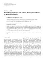
Figure 4: Node temperature.
least temperature from sender nodes to destination nodes
and avoid wasting the network bandwidth by reducing the
hop count. In other words, LTRT selects a least tempera-
ture route from all possible routes from a sender node to a
destination, not always choosing the least temperature sen-
sor nodes. In short, LTRT calculates routes from the single-
source shortest path algorithms in graph theory (e.g., Dijk-
stra’s algorithms) and applies these routes for later packet

transmissions. With our expectation, LTRT will be posi-
tioned just between LTR and SHR and more efficient than
ALTR. Therefore, like TARA, LTR, and ALTR, LTRT requires
every node to assure temperature of its neighboring nodes
from the received and transmitted packets.
To apply the single-source shortest path problem in
graph theory to the thermal-aware routing problem, our pro-
tocol follows the next four steps.
(1) Assign temperature of sensor nodes as weight to each
sensor node from observation of communication ac-
tivity by neighboring sensor nodes, shown in Figure 4.
(2) In calculating routes, transfer weight (temperature) of
sensor nodes to weight of edges ahead. For example,
supposing that u and v are vertices (nodes) in directed
graph G and (u, v) is an edge connecting vertices u and
v (i.e., u
→v), then w(u, v) (weight of (u, v)) is temper-
ature of vertex u. This transfer is shown in Figure 5.
Thus, upon transferring weight of each sensor node
to the corresponding edges, temperature of destination
nodes is just ignored.
(3) By using the second graph, apply single-source short-
est path algorithms to figure out routes having the least
temperature from sending nodes to destination nodes.
(4) To avoid excessively raising temperature of sensor
nodes, periodically maintaining (updating) routes is
required. The maintenance of routing also helps in
adapting frequent network topology changes caused
by node movements.
Figure 4 shows that from observing communication ac-

tivity of neighboring nodes (v1, v2, v3, and v4), weight (tem-
perature (t1, t2, t3, and t4)) of each sensor node can be calcu-
lated. At this point, temperature is just related to each sensor
node.
Figure 5 shows that eight sensor nodes are transferred to
corresponding directed edges ahead (e.g., t1andt2). Now,
v1 v2
v3 v4
t1 t2
t3 t4
t1
t2
t1
t2
t1
t2
v1 v2
v3 v4
t1 t2
t3 t4
t1
t2
t3
t4
t1
t2
t1
t3
t2
t4

t3
t4
Figure 5: Building weight graph.
every edge is weighed according to weights of sensor nodes,
and the edges come from constructing a weighted directed
graph.
One tradeoff of the proposed scheme is that it requires
sensor temperature to be transmitted among sensor nodes,
and this operational overhead causes the battery consump-
tion and temperature increase. Since the updating of sen-
sor temperature is done periodically and the number of
sensor nodes may not be large in the telemedicine appli-
cation, the overhead can be tolerated and indicated in our
simulations.
4. SIMULATIONS
To evaluate the temperature rise and the efficiency of power
consumption of each algorithm, we wrote the simulation
program by Java using discrete event simulation. Our simu-
lations mainly consist of four events: route generation, send-
ing packet, receiving packet, and periodically cooling down
the temperature of every sensor node in the network. In-
stead of sending packets to a fixed base station, we rather
choose the way in which the sender and the destination are
selected randomly by each packet generation so that they can
vary in every execution. We fixed the network topology as a
mesh topology so that every sensor node in the network can
be connected and send packets to any other node by using
multihopping. In this topology setting, the number of sensor
nodes can be changed so that we can measure the scalability
of each algorithm in terms of the number of sensor nodes as

well. The scalability is measured from 20 to 100 sensor nodes
byastepof10sensornodes.
Because of the simulation results from [1], at this time,
comparisons are made among only three thermal-aware
routing algorithms: the least total-route-temperature (LTRT,
proposed) algorithm, the least temperature routing (LTR) al-
gorithm, and the adaptive least temperature routing (ALTR)
algorithm. Our simulations are based upon the transition of
the increasing packet generation rate, where how many pack-
ets are generated in the unit time and the number of sensor
nodes in the network, and three metrics are designed to eval-
uate the efficiency of each algorithm: average temperature
rise, average hop count per arrival packet, where the met-
rics are interpreted into average delay of arrival packets, and
percentage of lost packets.
Daisuke Takahashi et al. 5
32.752.52.2521.751.51.2510.750.50.25
Packet generation rate
LT RT ( p r op o s e d )
LT R
ALTR
0
100
200
300
400
500
600
700
Average temperature rise

Packet generation rate versus average temperature rise, R = 30
Figure 6: Packet generation rate versus average temperature rise
with radio transmission range 30.
Each simulation continues iterating until totally 2000
packets are generated and either delivered to the destinations
or discarded (recorded as lost packets), for example, the sum
of the delivered packets and the lost packets reaches 2000.
The sensor node temperature rises by 1 unit when they re-
ceive a packet, and initially every node has 1 unit of temper-
ature. In these simulations, while we defined the minimum
temperature of the sensor node as 1 unit, the maximum tem-
perature was not defined or defined with infinity. Also, when
time passes the specified period, which was set to 40 units of
time in these simulations, the process reduces 1 unit of tem-
perature from every sensor node. Since we assume that the
power consumption will be in relation to the total hops per-
formed in the network, in the simulations, we did not mea-
sure the power consumption separately.
Furthermore, by following the simulation setting in [1],
we assume that the value of MAX
HOPS in LTR was equal
to 40 and MAX
HOPS ADAPTIVE in ALTR was 10 so that
ALTR would change the routing algorithm from LTR to the
shortest hop routing (SHR) algorithm at this threshold.
4.1. 5
×10 mesh topology
In the 5
× 10 mesh topology simulation, we fix the number
of sensor nodes equal to 50 while we increase the packet gen-

eration rate, where how many packets are generated per unit
time, from 0.25 to 3.0.
4.1.1. Packet generation rate versus average
temperature rise
When the radio transmission range is set to 30, since we set
the distance of two adjacent nodes to 20, every sensor node
has at least 3 neighboring nodes, where the nodes are at the
corner, and some of sensor nodes can have 8 neighboring
nodes. As shown in Figure 6, every of the three algorithms
has the similar tendency, that is, in relation to the packet gen-
eration rate, the average temperature rise grows faster in the
range of 0.25 to 1 while after this range, they tend to become
stable. However, since in LTR packets need to roam in the
network until either they can reach the destination or exceed
the predefined max hop count threshold, they keep the tem-
perature of the entire network comparatively high resulting
in the high average temperature. Instead, since our proposed
LTRT determines a route to the destination before starting
sending packets, it is impossible for packets to roam in the
network and this affects the number of total hop counts re-
quired to reach the destination and consequently influences
temperature rise of the entire network.
In case that the radio transmission range is 25, sensor
nodes in the network have at least 2 neighbors up to 4 neigh-
bors. In this case, the choice of the next sensor nodes for
the routing is apparently reduced, and the average tempera-
ture rise gets higher than the case that the radio transmission
range is 30. This is because, due to the reduction of the num-
ber of the neighbors, the probability that packets will arrive
at the destination gets lower within certain hop counts than

the case of the radio transmission range 30. Therefore, pack-
ets require extra travel around the network and consequently
it takes them more time to get to the destination, resulting in
raising the entire temperature. Thus, as the number of neigh-
boring nodes is reduced, the total temperature of the network
gets higher.
4.1.2. Packet generation rate versus hop
count per arrived packet
Next, we simulate the relation between the packet gener-
ation rate and hop count per arrived packet in regarding
three routing algorithms. This metric also can be translated
into the average cost or delay for packets to get to the des-
tination because as the number of hop counts increases, a
packet is apparently delivered to the destination in a longer
time.
From Figure 8, hop count per arrived packet does not
seem to have any relation to the packet generation rate. In-
stead, all three algorithms experience relatively stable hop
counts in the entire simulation.
However, the degree of the average hop count varies from
one algorithm to another. LTRT is, in general, designed to
choose a route in which the sum of the temperature of for-
warding sensor nodes is the least. Therefore, LTRT is con-
sidered to have advantages of both SHR and LTR, that is,
LTRT is considered as a hybrid of SHR and LTR. Since LTRT
is concerned with both the shortest hop count and the least
temperature, the average hop count is much lower than LTR
and ALTR. On the other hand, LTR initially does not know
the direction of the destination unless a sensor node hav-
ing a packet neighbor as the destination, and only concerns

about the temperature of the neighboring nodes but not
about the temperature of the total network. Thus, LTR is
apt to choose a neighboring node that has the least temper-
ature even though it is located opposite to the destination.
Therefore, while LTR raises the temperature of individual
sensor nodes a little, regarding the temperature of the en-
tire network, it raises the temperature higher and faster than
LT RT.
6 EURASIP Journal on Wireless Communications and Networking
32.752.52.2521.751.51.2510.750.50.25
Packet generation rate
LT RT ( p r op o s e d )
LT R
ALTR
0
100
200
300
400
500
600
700
800
900
Average temperature rise
Packet generation rate versus average temperature rise, R = 25
Figure 7: Packet generation rate versus average temperature rise
with radio transmission range 25.
32.752.52.2521.751.51.2510.750.50.25
Packet generation rate

LT RT ( p r op o s e d )
LT R
ALTR
0
2
4
6
8
10
12
14
16
18
20
Hop count per packet
Packet generation rate versus hop count per packet, R = 30
Figure 8: Packet generation rate versus hop count per arrived
packet.
4.1.3. Packet generation rate versus percentage of
thelostpacket
Regarding the total lost packets, shown in Figure 9, LTR has
relatively high ratio based on the total number of sending
packets, and this is easily explained by the result of the sim-
ulation of the packet generation rate versus hop counts per
arrived packet. The previous simulation showed us that LTR
takes packets more time to arrive at the destination, and this
increases the probability that packets exceed a predefined
maximum hop count threshold. Moreover, since LTRT and
ATLR are designed to send almost every packet to the des-
tination eventually, the percentage of the lost packets is very

close to zero.
4.2. Scalability simulation
In this simulation, we investigate the tendency of the temper-
ature rise, total hop counts per arrived packet, and percent-
32.752.52.2521.751.51.2510.750.50.25
Packet generation rate
LT RT ( p r op o s e d )
LT R
ALTR
0
2
4
6
8
10
12
14
16
Lost packet (%)
Packet generation rate versus % lost packet, R = 30
Figure 9: Packet generation rate versus percentage of lost packet.
10090807060
50
403020
Number of nodes
LT RT ( p r op o s e d )
LT R
ALTR
0
100

200
300
400
500
600
Average temperature rise
Number of nodes versus average temperature rise, R = 30
Figure 10: Number of sensor nodes versus average temperature
rise.
age of the lost packet in terms of the number of sensor nodes
in the network. The scalability is measured in the range of 20
to 100, and in each case, we simulate the temperature rise and
other metrics by operating the three thermal-aware routing
algorithms: LTR, ALTR, and LTRT.
4.2.1. Number of sensor nodes versus average
temperature rise
As the number of sensor nodes increases, since all the
three thermal-aware routing algorithms can disperse rout-
ings throughout the entire network, the average temperature
basically decreases. Therefore, ALTR and our proposed LTRT
represent this tendency well in Figure 10.InLTR,however,
the average temperature gradually increases as the number
of nodes increases up to 50 sensor nodes. This is because,
the more the number of nodes becomes, the more chances
the packets get to trace extra nodes whose temperature is
Daisuke Takahashi et al. 7
10090807060
50
403020
Number of nodes

LT RT ( p r op o s e d )
LT R
ALTR
0
5
10
15
20
25
30
35
40
Hop count per packet
Number of nodes versus hop count per packet, R = 30
Figure 11: Number of sensor nodes versus hop counts per arrived
packet.
comparatively low until arriving at the destination. In other
words, as the number of sensor nodes increases, the number
of choices of routes from the sender to the destination also
increases. Therefore, the packets are attempted to roam more
around the entire network, and this causes the temperature
of the entire network to become higher. Moreover, as the
number of nodes exceeds 50, the distance from the senders
to the destinations also becomes longer, and because pack-
ets tend to exceed a predefined hop count threshold, they are
dropped out of the network and cannot increase the route
temperature anymore so that the average temperature grad-
ually decreases.
4.2.2. Number of sensor nodes versus hop
counts per arrived packet

Figure 11 shows the tendency of the hop count rise based
on the number of sensor nodes. As we have already men-
tioned in the previous section, as the number of sensor
nodes grows, choices of routes from the sender to the des-
tination also increase. In general, this helps the tempera-
ture averaging over all the sensor nodes in the network de-
crease. In LTR, however, since packets always choose the least
temperature nodes until they arrive at the destination or
exceed a predefined threshold, directions are not necessar-
ily toward the destination. Thus, in LTR and ALTR, pack-
ets are attempted to select these low-temperature nodes in-
stead of directly going toward the destination nodes. In case
of a network with 100 sensor nodes, the number of hop
counts per arrived packet of LTR almost reaches 40. There-
fore, in 100 sensor nodes, almost all packets are discarded
from the network. One solution to avoid this situation is
to let the packets have more hop counts. However, since
this solution also allows packets to roam around the net-
work longer, the temperature of the entire network will also
increase.
1009080706050403020
Number of nodes
LT RT ( p r op o s e d )
LT R
ALTR
0
5
10
15
20

25
30
35
Lost packet (%)
Number of nodes versus % lost packet, R = 30
Figure 12: Number of sensor nodes versus percentage of lost packet
in case of radio transmission range 30.
1009080706050403020
Number of nodes
LT RT ( p r op o s e d )
LT R
ALTR
0
10
20
30
40
50
60
Lost packet (%)
Number of nodes versus % lost packet, R = 25
Figure 13: Number of sensor nodes versus percentage of lost packet
in case of radio transmission range 25.
4.2.3. Number of sensor nodes versus
percentage of lost packet
We investigate the relation between the number of sensor
nodes and lost packets out of 2000 generated packets. The
results are shown in Figures 12 and 13.InFigure 12, this is
the case that radio transmission range of each sensor node
is equal to 30 so that every node can have neighbors in the

range from 3 up to 8. Moreover, in Figure 13, their radio
transmission range is restricted up to 25 so that sensor nodes
have no more than 4 or less neighbors.
Both figures show the same tendency similar to that in
LTR, as the number of sensor nodes increases in the net-
work, the percentage of lost packet grows, and these results
8 EURASIP Journal on Wireless Communications and Networking
43.63.22.82.421.61.20.80.4
Δ temperature rise
LT RT ( p r op o s e d )
LT R
ALTR
0
500
1000
1500
2000
2500
3000
Average temperature rise
Δ temperature rise versus average temperature rise, R = 30
Figure 14: Δ temperature rise versus average temperature rise.
are explained in the previous simulation, that is, the num-
ber of sensor nodes versus hop counts per arrived packet. In
the previous simulation, as the number of sensor nodes in-
creases, the number of hop counts per arrived packet also in-
creases in LTR. Since as the number of hop counts increases,
the probability that packets exceed a predefined threshold
also gets higher, and this probability directly affects the per-
centage of lost packet.

Meanwhile, both ALTR and our proposed LTRT show
much efficiency about the lost packets that is close to zero. In
ALTR, routing algorithm can be changed from LTR to SHR,
whose objective is to send packets to the destination as soon
as possible, after packets exceed a predefined threshold. LTR
experiences much more lost packets than the other two al-
gorithms, where almost half of the sending packets are dis-
carded in case of radio transmission range 25. This tendency
just shows that the network is unreliable.
4.3. Δ temperature rise versus average
temperature rise
We investigate the relation between settings of Δ tempera-
ture rise and the average temperature rise in Figure 14.In
short, Δ temperature rise means how much temperature of
each node increases when it receives a packet from the neigh-
boring nodes. In previous simulations, we just set this value
to one temperature unit, which is constant. However, we fig-
ureoutthataswegraduallyincreasedΔ temperature, since
the total network temperature is calculated by the product
of Δ temperature rise and the total hop counts performed in
the network, the average temperature of the networks in LTR
and ALTR goes up faster than LTRT. Thus, from the applica-
tion perspective, reducing the total hop counts of each packet
is one solution to suppress the total or average temperature
rise of the network. In other words, how to control the total
hop count by routing algorithms is very
important.
100908070605040302010
Cool down interval
LT RT ( p r op o s e d )

LT R
ALTR
0
100
200
300
400
500
600
700
Average temperature rise
Cool down interval versus average temperature rise
Figure 15: Cool-down interval versus average temperature rise.
4.4. Cool-down interval versus average
temperature rise
Figure 15 shows the relation between the cool-down inter-
vals and average temperature rises. It shows how the aver-
age temperature rise will change when the cool-down inter-
val gets longer. Basically, each implementation of the simu-
lation takes around 2000 units of time. Thus, in case of set-
ting the cool-down interval with 5 units of time, the cool-
downs are conducted 400 times in each simulation, and this
can be translated that total 400 units of temperature are re-
duced from the total temperature or 8 units of temperature
are reduced from each node. On the other hand, when we set
the cool-down interval with 100 units of time, the simulation
experienced only 20 cool-down events, and this means that
totally no more than 20 units could be reduced from the total
temperature.
In general, every thermal-aware routing algorithm shows

ascent of its trend as the cool-down interval gets longer.
However, in Figure 15, in the first ascending trend, LTRT
shows relatively gentle temperature rise, while in LTR and
ALTR, the average temperatures witness a rapid increase by
more than 200 units. Therefore, although after these steep
rises of the average temperature both of the ascending trends
gradually slow down, both of LTR and ALTR record higher
average temperatures than that of LTRT.
This simulation shows us that the cool-down interval is
also an important parameter affecting the average temper-
ature of every sensor node. However, since this parameter
largely relies on inside temperature of the human bodies,
generally by no means, can this parameter be controlled by
the application of the biomedical sensors themselves.
4.5. Level of hot spot versus number of packets
passing hot spots
In Figure 16, we gradually change the point of the hot spot,
where the packet generation rate is 1 and the number of sen-
Daisuke Takahashi et al. 9
1100
1050
1000
950
900
850
800
750
700
650
600

550
500
450
400
350
300
250
200
150
100
Level of hot spot
SHR
LT R
ALTR
LT RT ( p r op o s e d )
0
5000
10000
15000
20000
25000
Number of packets passing hot spots
Level of hot spot versus number of packets passing hot spots
Figure 16: Level of hot spot versus number of packets passing hot
spots.
sor nodes is 50. The simulation starts with hot spot point 100,
which means that sensor nodes that have more than 100 units
of temperature are considered as hot spots. This hot spot
point is thought to be low because even LTRT experiences
about 100 units of the average temperature rise. Figure 16

shows that for every routing algorithm, packets experience
more or less hot spot passing. However, as we mentioned that
LTRT generates only about 100 units of the average temper-
ature, after we set the point of the hot spot with 100, almost
no packet experiences hot spot passing. Moreover, since LTR
and ALTR generate relatively high average temperatures, even
though the number of packets passing hot spots decreases,
packets are still required to choose hot spots on their rout-
ing paths even after the hot spot is set with 300. The previous
simulations show that LTR generates the average temperature
rise near 600 units of temperature, and packets keep experi-
encing hot spot passing up to hot spot set with 600.
For LTR and ALTR, when they generate the average tem-
perature more than the level of the hot spot, almost all sensor
nodes have temperature over the hot spot. However, this sit-
uation is critical in thermal-aware routing applications.
Our assumption is that fewer hop counts generate fewer
hot spots and consequently less average temperature. There-
fore, even the shortest hop routing (SHR) algorithm gener-
ates better performance than LTR and ALTR in terms of the
hot spot. However, since SHR concerns about the hop count
rather than temperature, even though it generates compar-
atively low average temperature rise, which is close to those
generated by LTRT, it still experiences the hot spot passing at
higher hot spot settings than that of LTRT.
4.6. Packet generation rate (PGR) versus percent of hot
spot passed by packets
Figure 17 presents the transition of how many hot spots
packets pass by as the packet generation rate increases. In this
simulation, a hot spot is set up with 300 units of temperature,

32.752.52.2521.751.51.2510.750.50.25
Packet generation rate
SHR
LT R
ALTR
LT RT ( p r op o s e d )
0
5
10
15
20
25
30
35
40
45
50
Hotspotpassedbypackets(%)
PGRversus%ofhotspotpassedbypackets,R = 30
Figure 17: Packet generation rate versus number of hot spots
passed by packets with radio transmission range 30.
and the ratio of the number of hot spots passed by packets
to the total hops is calculated. As we have mentioned in the
previous simulations, since the average temperature rise gets
higher as the packet generation rate increases, the probability
that packets choose routing paths which partially contain hot
spots also gets higher. Figure 17 just shows this tendency.
In LTRT, the average temperature rise is comparatively
low, which is no more than 150, and because of its nature of
avoidance of hot spots, no packet goes through hot spots in

the execution. On the other hand, although SHR generates
almost the same average temperature rise as those in LTRT,
packets still need to pass through hot spots in every execution
except for packet generation rate of 0.25, where they record
about 5% of the total hop count.
However, in LTR and ALTR, things get worse than SHR,
and about 45% and 20% of the total hops pass over the hot
spots, respectively. Since both of the algorithms experience
the higher average temperature rise, packets basically experi-
ence more hot spot passing even though they are attempted
to avoid passing hot spots by always choosing the least tem-
perature nodes. One weakness of these algorithms is that be-
cause the packets select the least temperature neighbor nodes
as their routing paths every time, the temperature of every
node evenly gets higher as the process goes on. Therefore,
when the average temperature exceeds a hot spot setting,
almost every node has temperature exceeding the hot spot
temperature. Consequently, the later probability that packets
will pass through hot spots becomes much higher than those
of LTRT and SHR.
4.7. Number of nodes versus percent of hot spot
passed by packets
As described in the previous simulations, the number of
nodes and the average temperature rise are, in general, in-
versely related. Therefore, as the number of nodes increases,
the ratio of the number of hot spots passed by packets to the
10 EURASIP Journal on Wireless Communications and Networking
1009080706050403020
Number of nodes
SHR

LT R
ALTR
LT RT ( p r op o s e d )
0
5
10
15
20
25
30
35
40
45
50
Hotspotpassedbypackets(%)
Number of nodes versus % hot spot passed by packets, R = 30
Figure 18: Packet generation rate versus percentage of hot spot
passed by packets with radio transmission range 30.
total hop count decreases. However, since LTR generates over
400 units of temperature rise even with 100 nodes, 1/3 of
hops are still required to pass over hot spots in LTR with 100
sensor nodes. On the other hand, after the number of nodes
exceeds 60, ALTR keeps its average temperature below 300.
Since then, no packet experiences hot spot passing.
Furthermore, although, as the number of nodes in-
creases, the probability that packets pass through the hot
spots gets lower, in SHR, the packets still have chances to se-
lect the hot spots as part of their routing paths. In the figure
above, occasionally SHR generates about 5% of the hot spot
passing even though in other cases, it becomes lower or none.

5. CONCLUSIONS
This paper proposed a thermal-aware routing algorithm
called the least total-routing-temperature (LTRT) algorithm
that mainly concerns about both the shortest hop count and
the least temperature rise of the entire network. It is a hybrid
of the shortest hop-count routing (SHR) algorithm and the
least temperature routing (LTR) algorithm described in [1].
Our thermal-aware routing algorithm is based on the single
source shortest path (SSSP) in the graph theory and is mod-
ified such that the temperature of sensor nodes is transferred
to the weight of out going edges so that the SSSP can choose
a route where the sum of temperatures of forwarding nodes
is the least. Since LTRT aims to send packets with nearly the
shortest hop counts, it prevents the entire network temper-
ature from rising quickly. Also, since LTRT concerns about
the total temperature of selected routes, instead of choos-
ing the shortest hop count routes having comparatively high
temperature, it is attempted to detour sensor nodes that have
high temperature and cause the route temperature to be high.
To evaluate the efficiency of our proposed algorithm,
we performed extensive simulations comparing LTRT with
LTR and the adaptive least temperature routing (ALTR) algo-
rithm [1] in terms of temperature rising or other efficiencies.
Our simulation results show that packets experience low hop
counts up to the destination compared with LTR and ALTR.
On the other hand, in LTR and ALTR, prior to a predefined
threshold, sender nodes always choose the least-temperature
neighbor node for their route so that packets can keep roam-
ing in the network in a longer period of time than SHR and
LTRT. Thus, in the simulations, both LTR and ALTR always

recorded higher temperature than the proposed LTRT. In ad-
dition, we also performed a couple of simulations in terms of
the scalability of all the three thermal-aware algorithms. In
these simulations, LTRT shows good performance in terms
of temperature rise, hop counts per arrival packet, and per-
centage of lost packets. LTR largely degrades its performance,
especially about the number of hop counts and lost packets.
In particular, in case of 100 sensor nodes, in LTR, almost half
of the generated packets are discarded due to an excess of hop
counts, and this, to a great extent, degrades the reliability of
the sensor network.
In our future research, we will keep exploring more de-
tails about the thermal-aware routing algorithms and also
design more optimal solutions or alternatives. Moreover, we
will design the architecture and real application with scenar-
ios adopting our proposed routing algorithm. The proposed
scheme can be used in remote cardiac patients monitoring
applications in [14, 15].
ACKNOWLEDGMENTS
This work is partially supported by the US National Sci-
ence Foundation (NSF) under Grants no. CNS-0716211 and
CNS-0716455. The work of Zhejiang University is partially
supported by the National Natural Science Foundation of
China (NSFC) under Grant no. 60604029, and by Joint
Funds of NSFC-Guangdong under Grant no. U0735003.
REFERENCES
[1] A. Bag and M. A. Bassiouni, “Energy efficient thermal aware
routing algorithms for embedded biomedical sensor net-
works,” in Proceedings of the 1st IEEE International Workshop
on Intelligent Systems Techniques for Wireless Sensor Network in

conjunction with the 3rd IEEE International Conference on Mo-
bile Ad-hoc and Sens or Systems, pp. 604–609, Vancouver, BC,
Canada, October 2006.
[2] L. Schwiebert, S. K. S. Gupta, and J. Weinmann, “Research
challenges in wireless networks of biomedical sensors,” in Pro-
ceedings of the 7th Annual International Conference on Mo-
bile Computing and Networking (MobiCom ’01), pp. 151–165,
Rome, Italy, July 2001.
[3] L. Schwiebert, S. K. S. Gupta, P. S. G. Auner, G. Abrams, R.
Iezzi, and P. McAllister, “A biomedical smart sensor for the vi-
sually impaired,” in Proceedings of the IEEE Sensors , vol. 1, pp.
693–698, Orlando, Fla, USA, June 2002.
[4] C. Furse, H. K. Lai, C. Estes, A. Mahadik, and A. Dun-
can, “An implantable antenna for communication with im-
plantable medical devices,” in Proceedings of the IEEE Anten-
nas and Propagation/ URSI International Symposium,Orlando,
Fla, USA, July 1999.
[5]C.Furse,R.Mohan,A.Jakayar,etal.,“Abiocompatiblean-
tenna for communication with implantable medical devices,”
in Proceedings of the IEEE International Symposium on Anten-
nas and Propagation, San Antonio, Tex, USA, June 2002.
Daisuke Takahashi et al. 11
[6]Q.Tang,N.Tummala,S.K.S.Gupta,andL.Schwiebert,
“TARA: thermal-aware routing algorithm for implanted sen-
sor networks,” in Proceedings of the 1st IEEE International Con-
ference on Distributed Computing in Sensor Systems (DCOSS
’05), vol. 3560 of Lecture Notes in Computer Science, pp. 206–
217, Marina del Rey, Calif, USA, June-July 2005.
[7] Y. Prakash, S. Lalwani, S. K. S. Gupta, E. Elsharawy, and
L. Schwiebert, “Towards a propagation model for wireless

biomedical applications,” in Proceedings of the IEEE Interna-
tional Conference on Communications (ICC ’03), vol. 3, pp.
1993–1997, Anchorage, Alaska, USA, May 2003.
[8] W. R. Heinzelman, A. Chandrakasan, and H. Balakrishnan,
“Energy-efficient communication protocol for wireless mi-
crosensor networks,” in Proceedings of the 33rd Hawaii Inter-
national Conference on System Sciences (HICSS ’00), vol. 8, p.
8020, Maui, Hawaii, USA, January 2000.
[9] V. Shankar, A. Natarajan, S. K. S. Gupta, and L. Schwiebert,
“Energy-efficient protocols for wireless communication in
biosensor networks,” in Proceedings of the 12th I EEE Interna-
tional Symposium on Personal, Indoor and Mobile Radio Com-
munications (PIMRC ’01), vol. 1, pp. D114–D118, San Diego,
Calif, USA, September 2001.
[10] Y. Xiao, X. Shen, B. Sun, and L. Cai, “Security and privacy
in RFID and applications in telemedicine,” IEEE Communi-
cations Magazine, vol. 44, no. 4, pp. 64–72, 2006.
[11] F.Hu,S.Kumar,andY.Xiao,“Towardsasecure,RFID/sensor
based tele-cardiology system,” in Proceedings of the 4th
IEEE Consumer Communications and Networking Conference
(CCNC ’07), pp. 732–736, Las Vegus, Nev, USA, January 2007.
[12] Y. Xiao and F. Hu, “Wireless telemedicine and M-heath,” in
Proceedings of the 4th IEEE Consumer Communications and
Networking Conference (CCNC ’07), pp. 727–731, Las Vegus,
Nev, USA, January 2007.
[13] Y. Xiao, D. Takahashi, and F. Hu, “Telemedicine usage and
potentials,” in Proceedings of the IEEE Wireless Communica-
tions and Networks Conference (WCNC ’07), pp. 2736–2740,
Kowloon, China, March 2007.
[14] F. Hu, M. Jiang, and Y. Xiao, “Low-cost wireless sensor net-

works for remote cardiac patients monitoring applications,”
2007, to appear in Wireless Communications and Mobile Com-
puting Journal.
[15] F. Hu, M. Jiang, L. Celentano, and Y. Xiao, “Robust medical ad
hoc sensor networks (MASN) with wavelet-based ECG data
mining,” 2007, to appear in Ad Hoc Networks.
[16] Y. Xiao and H. Chen, Eds., Mobile Telemedicine: A Computing
and Networking Perspective, Auerbach Publications, Taylor &
Francis, New York, NY, USA, 2007.
[17] Q. Alexander, Y. Xiao, and F. Hu, “Telemedicine for perva-
sive healthcare,” in Mobile Telemedicine: A Computing and Net-
working Perspective, Auerbach Publications, Taylor & Francis,
New York, NY, USA, 2008.
[18] L. Biggers, Y. Xiao, and F. Hu, “Conventional telemedicine,
wireless telemedicine, sensor networks, and case studies,” in
Mobile Telemedicine: A Computing and Networking Perspective,
Auerbach Publications, Taylor & Francis, New York, NY, USA,
2008.
[19] F. Hu, M. Lewis, and Y. Xiao, “Automated blood glucose
management techniques through micro-sensors,” in Mobile
Telemedic ine: A Computing and Networking Perspective,Auer-
bach Publications, Taylor & Francis, New York, NY, USA,
2008.
[20] D. Takahashi, Y. Xiao, and F. Hu, “A survey of security
in telemedicine with wireless sensor networks,” in Mobile
Telemedic ine: A Computing and Networking Perspective,Auer-
bach Publications, Taylor & Francis, New York, NY, USA,
2008.
[21] F. Hu, L. Celentano, and Y. Xiao, “Mobile secure tele-
cardiology based on wireless and sensor networks,” in Mo-

bile Telemedicine: A Computing and Networking Perspective
,
Auerbach Publications, Taylor & Francis, New York, NY, USA,
2008.
[22] D. Takahashi, Y. Xiao, F. Hu, and M. Lewis, “A survey of
insulin-dependent diabetes part I: therapies and devices,” to
appear in Internat ional Journal of Telemedicine and Applica-
tions.
[23] J. Chen, K. Cao, Y. Sun, Y. Xiao, and X. Su, “Continuous drug
infusion for diabetes therapy: a closed-loop control system de-
sign,” to appear in EURASIP Journal on Wireless Communica-
tions and Networking.