Báo cáo hóa học: " Research Article RRES: A Novel Approach to the Partitioning Problem for a Typical Subset of System Graphs" potx

Hindawi Publishing Corporation
EURASIP Journal on Embedded Systems
Volume 2008, Article ID 259686, 13 pages
doi:10.1155/2008/259686
Research Article
RRES: A Novel Approach to the Partitioning Problem
for a Typical Subset of System Graphs
B. Knerr, M. Holzer, and M. Rupp
Institute of Communications and Radio-Frequency Engineering, Faculty of Electrical Engineering and Information Technology,
Vienna University of Technology, 1040 Vienna, Austria
Correspondence should be addressed to B. Knerr,
Received 11 May 2007; Revised 2 October 2007; Accepted 4 December 2007
Recommended by Marco D. Santambrogio
The research field of system partitioning in modern electronic system design started to find strong advertence of scientists about
fifteen years ago. Since a multitude of formulations for the partitioning problem exist, the same multitude could be found in
the number of strategies that address this problem. Their feasibility is highly dependent on the platform abstraction and the
degree of realism that it features. This work originated from the intention to identify the most mature and powerful approaches
for system partitioning in order to integrate them into a consistent design framework for wireless embedded systems. Within
this publication, a thorough characterisation of graph properties typical for task graphs in the field of wireless embedded system
design has been undertaken and has led to the development of an entirely new approach for the system partitioning problem.
The restricted range exhaustive search algorithm is introduced and compared to popular and well-reputed heuristic techniques
based on tabu search, genetic algorithm, and the global criticality/local phase algorithm. It proves superior performance for a set
of system graphs featuring specific properties found in human-made task graphs, since it exploits their typical characteristics such
as locality, sparsity, and their degree of parallelism.
Copyright © 2008 B. Knerr et al. This is an open access article distributed under the Creative Commons Attribution License, which
permits unrestricted use, distribution, and reproduction in any medium, provided the original work is properly cited.
1. INTRODUCTION
It is expected that the global number of mobile subscribers
will reach more than three billion in the year 2008 [1].
Considering the fact that the field of wireless communica-
tionsemergedonly25yearsago,thisgrowthrateisabso-

lutely tremendous. Not only its popularity experienced such
a growth, but also the complexity of the mobile devices ex-
ploded in the same manner. The generation of mobile de-
vices for 3G UMTS systems is based on processors containing
more than 40 million transistors [2]. Compared to the first
generation of mobile phones, a staggering increase in com-
plexity of more than six orders of magnitude has taken place
[3] in the last 15 years. Unlike the popularity, the growing
complexity led to enormous problems for the design teams
to ensure a fast and seamless development of modern em-
bedded systems.
The International Technology Roadmap for Semicon-
ductors [4] reported a growth in design productivity, ex-
pressed in terms of designed transistors per staff month,
of approximately 21% compounded annual growth rate
(CAGR), which lags behind the growth in silicon complex-
ity. This is known as the design gap or productivity gap.A
broad range of reasons exist that hold responsible for the
design gap [5, 6]. The extreme heterogeneity of the applied
technologies in the systems adopts a predominant position
among those. The combination of computation-intensive
signal processing parts for ever higher data rates, a full
set of multimedia applications, and the multitude of stan-
dards for both areas led to a wild mixture of technologies
in a state-of-the-art mobile device: general-purpose proces-
sors, DSPs, ASICs, multibus structures, FPGAs, and ana-
log mixed signal domains may be coexisting on the same
chip.
Although a number of EDA vendors offer tool suites (e.g.,
ConvergenSC of CoWare, CoCentric System Studio of Syn-

opsys, Matlab/Simulink of The MathWorks) that claim to
cope with all requirements of those designs, some crucial
steps are still not, or inappropriately, covered: for instance,
the automatic conversion from floating-point to fixed-point
representation, architecture selection, as well as system par-
titioning [7].
2 EURASIP Journal on Embedded Systems
This work focuses on the problem of hardware/software
(hw/sw) partitioning, that is, loosely spoken, the mapping
of functional parts of the system description to architec-
tural components of the platform, while satisfying a set of
constraints like time, area, power, throughput, delay, and so
forth. Hardware then usually addresses the implementation
of a functional part, for example, performing an FIR or CRC,
as a dedicated hardware unit that features a high throughput
and can be very power efficient. On the other hand, a custom
data path is much more expensive to design and inflexible
when it comes to future modifications. Contrarily, software
addresses the implementation of the functionality as code to
be compiled for a general-purpose processor or DSP core.
This generally provides flexibility and is cheaper to maintain,
whereas the required processors are more power consuming
and offer less performance in speed. The optimal trade-off
between cost, power, performance, and chip area has to be
identified. In the following, the more general term system
partitioning is preferred to hw/sw partitioning, as the clas-
sical binary decision between two implementation types has
been overcome by the underlying complexity as well. The
short design cycles in the wireless domain boosted the de-
mand for very early design decisions, such as architecture

selection and system partitioning on the highest abstraction
level, that is, the algorithmic description of the system. There
is simply no time left to develop implementation alternatives
[5], which was used to be carried out manually by design-
ers recalling their knowledge from former products and esti-
mating the effects caused by their decision. The design com-
plexity exposed this approach unfeasible and forced research
groups to concentrate their efforts on automating the system
partitioning as much as possible.
For the last 15 years, system partitioning has been a re-
search field starting with first approaches being rather the-
oretic in their nature up to quite mature approaches with a
detailed platform description and a realistic communication
model. N.B., until now, none of them has been included in
any commercial EDA tool, although very promising strategies
do exist in academic surroundings.
In this work, a new deterministic algorithm is introduced
that addresses the hw/sw partitioning problem. The cho-
sen scenario follows the work of other well-known research
groups in the field, namely, Kalavade and Lee [8], Wiangtong
et al. [9], and Chatha and Vemuri [10]. The fundamental idea
behind the presented strategy is the exploitation of distinct
graph properties like locality and sparsity, which are very typ-
ical for human-made designs. Generally speaking, the algo-
rithm locally performs an exhaustive search of a restricted
size while incrementally stepping through the graph struc-
ture. The algorithm shows strong performance compared to
implementations of the genetic algorithm as used by Mei et
al. [11], the penalt y reward tabu search proposed by Wiang-
tong [9], and the GCLP algorithm of Kalavade [8] for the

classical binary partitioning problem. And a discussion of its
feasibility is given with respect to the extended partitioning
problem.
The rest of the paper is organised as follows. Section 2
lists the most reputed work in the field of partitioning tech-
niques. Section 3 illustrates the basic principles of system
SW local
memory
General
purpose
SW processor
Register
HW-SW
shared
memory
System
bus
HW local
memory
Custom
HW
processor
Register
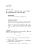
Figure 1:Commonplatformabstraction.
partitioning, gives an overview of typical graph representa-
tions, and introduces the common platform abstraction. It
is followed by a detailed description of the proposed algo-
rithm and an identification of the essential graph properties
in Section 5.InSection 6, the sets of test graphs are intro-
duced and the results for all algorithms are discussed. The

work is concluded and perspectives to future work are given
in Section 7.
2. RELATED WORK
This section provides a structured overview of the most in-
fluential approaches in the field of system partitioning. In
general, it has to be stated that heuristic techniques domi-
nate the field of partitioning. Some formulations have been
proved to be NP complete [12], and others are in P [13].
For the most formulations of partitioning problems, espe-
cially when combined with a scheduling scenario, no such
proofs exist, so they are just considered as hard.
In 1993, Ernst et al. [14] published an early work on the
partitioning problem starting from an all-software solution
within the COSYMA system. The underlying architecture
model is composed of a programmable processor core, mem-
ory, and customised hardware (Figure 1). The general strat-
egy of this approach is the hardware extraction of the compu-
tational intensive parts of the design, especially loops, on a
fine-grained basic block level, until all timing constraints are
met. These computation intensive parts are identified by sim-
ulation and profiling. Internally, simulated annealing (SA) is
utilised to generate different partitioning solutions. In 1993,
this granularity might have been feasible, but the growth in
system complexity rendered this approach obsolete. How-
ever, simulated annealing is still eligible if the granularity is
adjusted, to serve as a first benchmark provider due to its
simple and quickly to implement structure.
In 1995, the authors Kalavade [12] published a fast al-
gorithm for the partitioning problem. They addressed the
coarse grained mapping of processes onto an identical ar-

chitecture (Figure 1) starting from a directed acyclic graph
(DAG). The objective function incorporates several con-
straints on the available silicon area (hardware capacity),
B. Knerr et al. 3
memory (software capacity), and latency as a timing con-
straint. The global criticality/local phase (GCLP) algorithm is
basically a greedy approach, which visits every process node
once and is directed by a dynamic decision technique consid-
ering several cost functions.
In the work of Eles et al. [15], a tabu search algorithm
is presented and compared to simulated annealing and a
Kernighan-Lin (KL) based heuristic. The target architecture
does not differ from the previous ones. The objective func-
tion concentrates more on a trade-off between the commu-
nication overhead between processes mapped to different re-
sources and a reduction of execution time gained by paral-
lelism. The most important contribution is the preanalysis
before the actual partitioning starts. Static code analysis tech-
niques down to the operational level are combined with pro-
filing and simulation to identify the computation intensive
parts of the functional code. A suitability metric is derived
from the occurrence of distinct operation types and their dis-
tribution within a process, which is later on used to guide the
mapping to a specific implementation technology.
In the later nineties, research groups started to put more
effort into combined partitioning and scheduling techniques.
One of the first approaches to be mentioned of Chatha and
Ve m u r i [ 16] features the common platform model depicted
in Figure 1. Partitioning is performed in an iterative manner
on system level with the objective of minimising execution

time while maintaining the area constraint. The partition-
ing algorithm mirrors exactly the control structure of a clas-
sical Kernighan-Lin implementation adapted to more than
two implementation techniques, that is, for both hardware
and software exist more than one implementation type. Ev-
ery time a node is tentatively moved to another implemen-
tation type, the scheduler estimates the change in the over-
all execution time instead of rescheduling the task graph. By
this means, a low runtime is preserved by losing reliability of
their objective function since the estimated execution time
is only an approximation. The authors extended their work
towards combined retiming, scheduling, and partitioning of
transformative applications, for example, JPEG or MPEG de-
coder [10].
A very mature combined partitioning and scheduling ap-
proach for directed acyclic graphs (DAG) has been published
in 2002 by Wiangtong et al. [9]. The target architecture ad-
heres to the concept given in Figure 1,butfeaturesamore
detailed communication model. The work compares three
heuristic methods to traverse the search space of the par-
titioning problem: simulated annealing, genetic algorithm,
and tabu search. Additionally, the most promising technique
of this evaluation, tabu search, is further improved by a so-
called penalty reward mechanism. A reimplementation of
this algorithm confirms the solid performance in compar-
ison to the simulated annealing and genetic algorithms for
larger graphs.
Approaches based on genetic algorithms have been used
extensively in different partitioning scenarios: Dick and
Jha [17] introduced the MOGAC cosynthesis system for

combined partitioning/scheduling for periodic acyclic task
graphs, Mei et al. [11] published a basic GA approach for the
binary partitioning in a very similar setting to our work, and
Zou et al. [18] demonstrated a genetic algorithm with a finer
granularity (control flow graph level) but with the common
platform model of Figure 1.
3. SYSTEM PARTITIONING
This section covers the fundamentals of system partitioning,
the graph representation for the system, and the platform ab-
straction. Due to limited space, only a general discussion of
the basic terms is given in order to ensure a sufficient under-
standing of our contribution. For a detailed introduction to
partitioning, please refer to the literature [19, 20].
3.1. Graph representation of
signal processing systems
A common ground of modern signal processing systems is
their representation in dependence on their nature as data-
flow-oriented systems on a macroscopic level, for instance,
in opposition to a call graph representation [21]. Nearly ev-
ery signal processing work suite offers a graphical block-
based design environment, which mirrors the movement of
data, streamed or blockwise, while it is being processed [22–
24]. The transformation of such systems into a task graph
is therefore straightforward and rather trivial. To be in ac-
cordance with most of the partitioning approaches in the
field, we assume a graph representation to be in the form
of synchronous data flow graphs (SDF), that has been firstly
introduced in 1987 [25]. This form established the back-
bone of renowned signal processing work suites, for example,
Ptolemy [23]orSPW[22]. It captures precisely multiple in-

vocations of processes and their data dependencies and thus
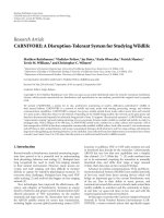
is most suitable to serve as a system model. In Figure 2(a),
a simple example of an SDF graph G
= (V, E) is depicted
that is composed of a set of vertices V
={a, , e} and a set
of edges E
={e
1
, , e
5
}. The numbers on the tail of each
edge e
i
represent the number of samples produced per invo-
cation of the vertex at the edge’s tail, out(e
i
). The numbers on
the head of each edge indicate the number of samples con-
sumed per invocation of the vertex at the edge’s head, in(e
i
).
According to the data rates at the edges, such a graph can be
uniquely transformed into a single activation graph (SAG)
in Figure 2(b). Every vertex in an SAG stands for exactly one
invocation of the process, thus the complete parallelism in
the design becomes visible. Here, vertex b and d occur twice
in the SAG to ensure a valid graph execution, that is, every
produced data sample is also consumed. The vertices cover
the functional objects of the system, or processes, whereas the

edges mirror data transfers between different processes.
Most of the partitioning approaches in Section 2 premise
the homogeneous, acyclic form of SDF graphs, or they state to
consider simply DAGs. An SDF graph is called homogeneous
if for all e
i
∈ E ,out(e
i
) = in(e
i
). Or in other words, the SDFG
and SAG exhibit identical structures. We explicitly allow for
general SDF graphs in our implementations of GA, TS, and
the new proposed algorithm. The transformation of general
SDF graphs into homogeneous SAG graphs is described in
[26], and does only affect the implementation complexity of
the mechanism that schedules a given partitioning solution
4 EURASIP Journal on Embedded Systems
a
b
d
c
e
1111
2
22
2
4
4
e

1
e
2
e
3
e
4
e
5
(a)
a
b
1
c
d
1
e
1
1
1
1
2
2
4
b
2
d
2
(b)
Figure 2: Simple example of a synchronous data flow graph and its decomposition into a single activation graph.

Shared
system
memory
(RAM)
DSP
(ARM)
Local SW
memory
DMA
DSP
(StarCore)
Local SW
memory
System bus
ASIC ASIC
Direct I/O
···
(a)
Shared
system
memory
(RAM)
DSP
(ARM)
Local SW
memory
DMA
Local HW memory
FPGA
System

bus
FPGA
block
FPGA
block
Direct I/O
···
(b)
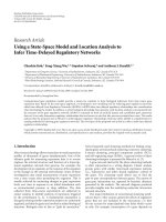
Figure 3: Origin (a) and modification (b) towards the common platform abstraction used for the algorithm evaluation.
onto a platform model. Note that due to its internal struc-
ture, the GCLP algorithm can not easily be ported to general
SDF graphs and so it has been tested to acyclic homogeneous
SDF graphs only.
In its current state, such a graph only describes the math-
ematical behaviour of the system. A binding to specific values
for time, area, power, or throughput can only be performed
in combination with at least a rough idea of the architecture,
on which the system will be implemented. Such a platform
abstraction will be covered in the following section.
3.2. Platform abstraction
The inspiration for the architecture model in this work origi-
nates from our experience with an industry-designed UMTS
baseband receiver chip [27]. Its abstraction (see Figure 3(a))
has been developed to provide a maximum degree of gen-
erality while being along the lines of the industry-designed
SoCs in use. The real reference chip is composed of two DSP
cores for the control-oriented functionality (an ARM for the
signalling part and a StarCore for the multimedia part). It
features several hardware accelerating units (ASICs), for the
more data-oriented and computation intensive signal pro-

cessing, one system bus to a shared RAM for mixed resource
communication, and optionally direct I/O to peripheral sub-
systems.
In Figure 3(b), the modification towards the platform
concept with just one DSP and one hardware processing unit
(e.g., FPGA) has been established (compare to Figure 1). This
modification was mandatory for the comparison to the parti-
tioning techniques of Wiangtong et al. [9] and Kalavade and
Lee [8].
To the best of our knowledge, Wiangtong et al. [9]
were the first group to introduce a mature communication
model with high degree of realism. They differentiate be-
tween load and store accesses for every single memory/bus
resource, and ensure a static schedule that avoids any col-
lisions on the communication resources. Whereas, for in-
stance, in the work of Kalavade [12], the communication
between processes on the same resource is neglected com-
pletely, in the works of Chatha and Vemuri [10]orVahid
and Le [21], the system’s execution time is estimated by av-
eraging over the graph structure, and Eles et al. [15]donot
generate a value for the execution time of the system at all,
but base their solution quality mainly on the minimisation
of communication between the hardware and the software
resources.
Since, in this work, the achievable system time is con-
sidered as one of the key system traits, for which constraints
exist, a reliable feedback on the makespan of a distinct par-
titioning solution is obligatory. Therefore, we adhere to a
detailed communication model. Tabl e 1 provides the exam-
ple access times for reading and writing bits via the differ-

ent resources of the platform in Figure 3(b). Communica-
tion of processes on the same resource uses preferably the
local memory, unless the capacity is exceeded. Processes on
different resources use the system bus to the shared mem-
ory. The presence of a DMA controller is assumed. In case
B. Knerr et al. 5
the designer already knows the bus type, for example, ARM
AMBA 2.0, the relevant values could be modified accord-
ingly.
With the knowledge about the platform abstraction de-
scribed in Section 3.2 the system graph is enriched with ad-
ditional information. The majority of the approaches assigns
a set of characteristic values to every vertex as follows:
∀v
i
∈ V ∃I(v
i
) =

et
H
, et
S
, gc,

,(1)
where et
H
is the execution time as a hardware unit, et
S

is the
execution time of the software implementation, and gc is the
gate count for the hardware unit and others like power con-
sumption and so forth. Those values are mostly obtained by
high-level synthesis [8] or estimation techniques like static
code analysis [28, 29] or profiling [30, 31]. Unlike in the
classical binary partitioning problem, in which just two im-
plementation types for every process exist (et
H
, et
S
), a set of
implementation types for every process is considered, com-
parable to the scenario chosen by Kalavade and Lee [8]and
Chatha and Vemuri [10]. This is usually referred to as an ex-
tended partitioning problem. Mentor Graphics recently re-
leased the high-level synthesis tool, CatapultC [32], which
allows for a fast synthesis of C functions for an FPGA or
ASIC implementation. By a variation of parameters, for ex-
ample, the unfolding factor, pipelining, or register usage, it
is possible to generate a set of implementation alternatives
A
i
FPGA
={gc,et} for every single process v
i
, like an FIR, fea-
tured by the consumed area in gates, the gate count gc,and
the execution time et. Accordingly, for every other resource,
like the ARM or the StarCore (SC) processors, sets of imple-

mentation alternatives, A
i
ARM
={cs, et} and A
i
SC
={cs, et},
can be generated by varying the compiler options. For in-
stance, the minimisation of DSP stall cycles is traded off
against the code size cs for a lower execution time et as fol-
lows:
∀v
i
∈ V ∃I
v
(v
i
) =

A
i
FPGA,1
, A
i
FPGA,2
, , A
i
FPGA,k
,
A

i
ARM,1
, A
i
ARM,2
, , A
i
ARM,l
,
A
i
SC,1
, A
i
SC,2
, , A
i
SC,m

.
(2)
In a similar fashion, the transfer times tt for the data trans-
fer edges e
i
are considered since several communication re-
sources exist in the design: the bus access to the shared mem-
ory (shr), the local software (lsm), and the local hardware
memory (lhm) as follows:
∀e
i

∈ E ∃I
e
(e
i
) =

tt
i
shr
, tt
i
lsm
, tt
i
lhm

. (3)
The next section finally introduces the partitioning problem
for the given system graph and the platform model under
consideration of distinct constraints.
3.3. Basic terms of the partitioning problem
In embedded system design, the term partitioning combines
in fact two tasks: allocation, that is, the selection of architec-
Table 1: Maximum throughput for read/write accesses to the com-
munication/memory resources.
Communication Read (bits/μs) Write (bits/μs)
Local software memory 512 1024
Local hardware memory 2048 4096
Shared system bus 1024 2048
Direct I/O 4096 4096

tural components, and mapping, that is, the binding of sys-
tem functions to these components. Since in most formula-
tions, the selection of architectural components is presumed,
it is very common to use partitioning synonymously with
mapping. In the remaining work, the latter will be used to
be more precise. Usually, a number of requirements, or con-
straints, are to be met in the final solution, for instance, ex-
ecution time, area, throughput, power consumption, and so
forth. This problem is in general considered to be intractable
or hard [33]. Arato et al. gave a proof for the NP com-
pleteness, but in the same work, they showed that other for-
mulations are in P [13].Ourworkelaboratesonsuchan
NP-partitioning scenario combined with a multiresource
scheduling problem. The latter has been proven to be NP-
complete [34, 35].
With the platform model given in Section 3.2, the alloca-
tion has been established. In Figure 4, the mapping problem
of a simple graph is depicted. The left side shows the system
graph, Figure 4(a), the right side shows the platform model
in a graph-like fashion, Figure 4(b). With the connecting arcs
in the middle, the system graph and the architecture graph
compose the mapping graph. The following constraints have
to be met to build a valid mapping graph.
(i) All vertices of the system graph have to be mapped to
processing components of the architecture graph.
(ii) All edges of the system graph have to be mapped to
communication components of the architecture graph
as follows.
(a) Edges that connect vertices mapped to an identi-
cal processing component have to be mapped to

the local communication component of this pro-
cessing component.
(b) Edges connecting vertices mapped to different
processing components have to be mapped to the
communication component, that connects these
processing components.
(iii) Communication components are either sequential or
concurrent devices. If read or write accesses cannot oc-
cur concurrently, then a schedule for these access op-
erations is generated.
(iv) Processing components can be sequential or concur-
rent devices. For sequential devices a schedule has to
exist.
A mapping according to all these rules is called feasible.How-
ever, feasibility does not ensure validity. A valid mapping is a
feasible mapping that fulfills the following constraints.
6 EURASIP Journal on Embedded Systems
a
b
c
d
e
e
1
e
3
e
5
e
4

e
2
SW
mem.
RISC
Bus
FPGA
HW
mem.
(a)Systemgraph (b)Architecturegraph
Figure 4: Mapping specification between system graph and archi-
tecture graph.
(i) A deadline T
limit
measured in clock cycles (or μs) must
not be exceeded by the makespan of the mapping so-
lution.
(ii) Sequential processing devices have a limited instruc-
tion or code size capacity C
limit
measured in bytes,
which must not be exceeded by the required memory
of mapped processes.
(iii) Concurrent processing devices have a limited area ca-
pacity A
limit
measured in gates, which must not be ex-
ceeded by the consumed area of the mapped processes.
Other typical constraints, which have not been considered in
this work in order to be comparable to the algorithms of the

other authors, are monetary cost, power consumption, and
reliability.
Due to the presence of sequential processing elements,
bus or DSP, the mapping problem includes another hard op-
timisation challenge: the generation of optimal schedules for
a mapping instance. For any two processes mapped to the
DSP or data transfers mapped to the bus that overlap in time,
a collision has to be solved. A very common strategy to solve
occurring collisions in a fast and easy-to-implement manner
is the deployment of a priority list introduced by Hu [36],
which will be used throughout this work. As our focus lies on
the performance evaluation of a mapping algorithm, a review
of different scheduling schemes is omitted here. Please refer
to the literature for more details on scheduling algorithms in
similar scenarios [37–39].
4. SYSTEM GRAPHS PROPERTIES, COST FUNCTION,
AND CONSTRAINTS
This section deals with the identification of system graph
characteristics encountered in the partitioning problem. A
set of properties is derived, which disclose the view to
promising modifications of existing partitioning strategies
and finally initiate the development of a new powerful par-
titioning technique. The latter part introduces the cost func-
tion to assess the quality of a given partitioning solution and
the constraints such a solution has to meet.
4.1. Revision of system graph structures
The very first step to design a new algorithm lies in the ac-
quisition of a profound knowledge about the problem. A re-
view of the literature in the field of partitioning and elec-
tronic system design in general, regarding realistic and gen-

erated system graphs has been performed. The value ranges
of the properties discussed below have been extracted from
the three following sources:
(i) an industry design of a UMTS baseband receiver chip
[27] written in COSSAP/C++;
(ii) a set of graph structures has been taken from Ra-
dioscape’s RadioLab3G, which is a UMTS library for
Matlab/Simulink [40];
(iii) three realistic examples stem from the standard task
graph set of the Kasahara Lab [41].
Additionally, many works incorporate one or two example
designs taken from development worksuites they lean to-
wards [8, 14]. Others introduce a fixed set of typical and very
regular graph types [9, 39]. Nearly all of the mentioned ap-
proaches generate additional sets of random graphs up to
hundreds of graphs to obtain a reliable fundament for test
runs of their algorithms. However, truly random graphs, if
not further specified, can differ dramatically from the specific
properties found in human made graphs. Graphs in elec-
tronic system design, in which programmers capture their
understanding of the functionality and of the data flow, can
be isolated by specific values for the following set of graph
properties.
Granularity
Depending on the granularity of the graph representation,
the vertices may stand for a single operational unit (MAC,
Add, or Shift) [14] or have the rich complexity of an MPEG
or H.264 decoder. The majority of the partitioning ap-
proaches [8–10, 17] decide for medium-sized vertices that
cover the functionality of FIRs, IDCTs, Walsh-Hadamards

transform, shellsort algorithms, or similar procedures. This
size is commonly considered as partitionable. The following
graph properties are related to system graphs with such a
granularity.
Locality
In graph theory, the term k-locality is defined as follows
[42]: a locality of k>0 means that when all vertices of a
graph are written as elements of a vector with indices i
=
1 |V|, edges may only exist between vertices whose indices
do not differ by more than k.Moredescriptively,human-
made graphs in electronic system design reveal a strong affin-
ity to this locality property for rather small k values com-
pared to its number of vertices
|V|. From a more pragmatic
perspective,itcanbeexpressedasagraph’saffinity to rather
short edges, that is, vertices are connected to other vertices
on a similar graph level. The generation of a k-locality graph
is simple but the computation of the k-locality for a given
graph is a hard optimisation problem itself, since k should be
B. Knerr et al. 7
r
loc
= 13/13 = 1
01234
(a)
r
loc
= 21/13 = 1.61
01 2 34

(b)
Figure 5: Examples for the rank-locality of two different graphs ac-
cording to (4).
(a) dense (b) sparse
Figure 6: Density of graph structures.
the smallest possible. Hence, we introduce a related metric to
describe the locality of a given graph: the rank-locality r
loc
.
In Figure 5, two graphs are depicted. At the bottom, the rank
(or precedence) levels are annotated and the rank-locality is
computed as follows:
r
loc
=
1
|E |

e
i
∈E
rank

v
sink
(e
i
)

−

rank

v
source
(e
i
)

. (4)
The rank-locality can be calculated very easily for a given
graph. Very low values, r
loc
∈ [1.0 2.0], are reliable indi-
cators for system graphs in signal processing.
Density
A directed graph is considered as dense if
|E |∼|V|
2
,andas
sparse if
|E |∼|V| [42], see Figure 6. Here, an edge corre-
sponds to a directed data transfer, which is either existing be-
tween two vertices or not. The possible values for the num-
ber of edges calculate to (
|V|−1) ≤|E |≤(|V|−1)|V |,
and for directed acyclic graphs to (
|V|−1) ≤|E |≤(|V|−
1)|V|/2. The considered system graphs are biased towards
sparse graphs with a density ratio of about ρ
=|E |/|V|=

2

|V|.
Degree of Parallelism
The degree of parallelism γ is in general defined as γ
=
|
V|/|V
LP
|,with|V
LP
| being the number of vertices on the
longest (critical) path [43]. In a weighted graph scenario this
definition can easily be modified towards the fraction of the
overall sum of the vertices’ (and edges’) weights divided by
ρ =
22
16
= 1.375 γ =
16
8
= 2 r
loc
=
27
22
= 1.227
01234567
Figure 7: Task graph with characteristic values for ρ, r
loc

,andγ.
the sum of the weights of the vertices (and edges) encoun-
tered on the longest path. Apparently, this modification fails
when the vertices and edges feature a set of varying weights
since in our case, the execution times et and transfer times tt
will serve as weights.
Hence, for every vertex and every edge an average is built
over their possible execution and transfer times, et
avg
and
tt
avg
. These averaged values then serve as unique weights for
the time-related degree of parallelism γ
t
:
γ
t
=

v
i
∈V
et
i
avg
+

e
j

∈E
tt
j
avg

v
i
∈V
LP
et
i
avg
+

e
j
∈E
LP
tt
j
avg
. (5)
This property may vary to a higher degree since many chain-
like signal processing systems exist as well as graphs with
a medium, although rarely high, inherent parallelism, γ
t
=
2

|V|. But for directed acyclic graphs this property can

be calculated efficiently beforehand and serves as a funda-
mental metric that influences the choice of scheduling and
partitioning strategies.
Taking these properties into account, random graphs of
various sizes have been generated building up sets of at least
180 different graphs of any size.
A categorisation of the system graph according to the
aforementioned properties for directed acyclic graphs can be
efficiently achieved by a single breadth-first search as follows:
(i) the totalised values for area A
total
, S
total
,andtimeT
total
;
(ii) the time based degree of parallelism γ
t
.
(iii) the ranks of all vertices;
(iv) the density ρ of the system graph.
These values can be achieved with linear algorithmic com-
plexity O(
|V| + |E |). A second run over the list of edges
yields the rank-locality property in O(
|E |). The set of pre-
conditions for the application of the following algorithm is
comprised by a low to medium degree of parallelism γ
t
∈

[2, 2

|V|], a low rank-locality r
loc
≤ 8, and a sparse density
ρ
= 2

|V|.
In Figure 7, a typical graph with low values for ρ and r
loc
is depicted. The rank levels are annotated at the bottom of the
graphic. The fundamental idea of the algorithm explained in
Section 5 is that, in general, a local optimal solution, for in-
stance, covering the rank levels 0 and 1, does probably not
interfere with an optimal solution for the rank levels 6 and 7.
8 EURASIP Journal on Embedded Systems
4.2. Cost function, constraints, and
performance metrics
Although there are about as many different cost functions as
there are research groups, all of the referred to approaches in
Section 2 consider time and area as counteracting optimisa-
tiongoals.Ascanbeseenin(6), a weighted linear combi-
nation is preferred due to its simple and extensible structure.
We have also applied Pareto point representations to seize the
quality of these multiobjective optimisation problems [44],
but in order to achieve comparable scalar values for the dif-
ferent approaches, the weighted sum seems more appropri-
ate. According to Kalavade’s work, code size has been taken
into account as well. Additional metrics, for instance, power

consumption per process implementation type, can just be
added as a fourth linear term with an individual weight. The
quality of the obtained solution, the cost value Ω
P
for the best
partitioning solution P, is then
Ω
P
=p
T
(T
P
) α
T
P
−T
min
T
limit
−T
min
+p
A
(A
P
) β
A
P
A
limit

+p
S
(S
P
) ξ
S
P
S
limit
.
(6)
Here, T
P
is the makespan of the graph for partitioning P,
which must not exceed T
limit
; A
P
is the sum of the area of
all processes mapped to hw, which must not exceed A
limit
; S
P
is the sum of the code sizes of all processes mapped to sw,
which must not exceed S
limit
. With the weight factors α, β,
and ξ, the designer can set individual priorities. If not stated
otherwise, these factors are set to 1. In the case that one of
the values T

P
, A
P
,orS
P
exceeds its limit, a penalty function
is applied to enforce solutions within the limits:
p
A

A
P
A
limit

=
⎧
⎪
⎪
⎨
⎪
⎪
⎩
1.0, A
P
≤ A
limit
,

A

P
A
limit

η
, A
P
>A
limit
.
(7)
The penalty functions for p
T
and p
S
are defined analogously.
If not stated otherwise, η is set to 4.0.
The boolean validity value V
P
of an obtained partitioning
P is given by the boolean term: V
P
= (T
P
≤ T
limit
) ∧ (A
P
≤
A

limit
)∧(S
P
≤ S
limit
). A last characteristic value is the validity
percentage Ψ
= N
valid
/N, which is the quotient of the number
of valid solutions N
valid
divided by the number of all solutions
N, for a graph set containing N different graphs.
The constraints can be further specified by three ratios
R
T
, R
A
,andR
S
to give a better understanding of their strict-
ness. The ratios are obtained by the following equations:
R
T
=
T
limit
−T
min

T
total
−T
min
, R
A
=
A
limit
A
total
, R
S
=
S
limit
S
total
. (8)
The totalised values for area A
total
,codesizeS
total
,andexecu-
tion time T
total
are simply built by the sum of the maximum
gate counts gc, maximum code sizes cs, and maximum exe-
cution time et
max

of every process (plus the maximum trans-
fer time tt
max
of every edge), respectively. The computation
of T
min
is obtained by scheduling the graph under the as-
sumption of an implementation featuring a full parallelism,
that is, unlimited FPGA resources and no conflicts on any
a
c
bd
f
e
ih
g
j
k
m
l
n
Finally
mapped
RRES
window
Te n t a t i v e l y
mapped
Ordered vertex vector
Figure 8: Moving window for the RRES on an ordered vertex vec-
tor.

a
b
c
d
e
f
h
g
i
j
k
m
l
n
a
b
c
d
f
e
g
h
j
i
k
m
l
n
ASAP
a

c
bd
h
j
f
ik
l
n
m
g
e
ALAP
st
asap
(b) st
alap
(b)
Figure 9: Two different start times for process (b) according to
ASAP and ALAP schedule.
sequential device. It has to be stated that T
min
and T
total
are
lower and upper bounds since their exact calculation in most
cases is a hard optimisation problem itself.
Consequently, a constraint is rather strict when the al-
lowed for resource limit is small in comparison to the re-
source demands that are present in the graph. For instance,
the totalised gate count A

total
of all processes in the graph is
100k gates, if A
limit
= 20k, then R
A
= 0.2, which is rather
strict, as in average, only every fifth process may be mapped
to the FPGA or may be implemented as an ASIC.
The computational runtime Θ has been evaluated as well
andismeasuredinclockcycles.
5. THE RESTRICTED RANGE EXHAUSTIVE
SEARCH ALGORITHM
This section introduces the new strategy to exploit the prop-
erties of graph structures described in Section 4.1. Recall the
fundamental idea sketched in the properties section of non-
interfering rank levels. Instead of finding proper cuts in the
graph to ensure such a noninterference, which is very rarely
possible, we consider a moving window (i.e., a contiguous
subset of vertices) over the topologically sorted vertices of
the graph, and apply exhaustive searches on these subsets,
as depicted in Figure 8. The annotations of the vertices re-
fer to Figure 9. The window is moved incrementally along
the graph structure from the start vertices to the exit vertices
while locally optimising the subset of the RRES window.
The preparation phase of the algorithm comprises sev-
eral necessary steps to boost the performance of the proposed
B. Knerr et al. 9
Table 2: Averaged cost Ω
P

obtained for RRES starting from differ-
ent initial solutions.
Initial
solution
|V|
Pure
SW
Pure HW
Random Heuristic
Heuristic
and RRES
20 2.241 2.267
2.118 2.101
2.085
50 2.569 2.566
2.237 2.185
2.170
100 2.700 2.655
2.261 2.202
2.188
strategy. The initial solution, the very first assignment of
vertices to an implementation type, has an impact on the
achieved quality, although we can observe that this effect is
negligible for fast and reasonable techniques to create ini-
tial solutions. In Tabl e 2 , the obtained cost values for an
RRES (window length
= 8, loose constraints) are depicted
with varying initial solutions: pure software, pure hardware,
guided random assignment according to the constraint set-
ting, a more sophisticated but still very fast construction

heuristic described in the literature [45], and when apply-
ing RRES on the partitioning solutions obtained by a pre-
ceding run with the aforementioned construction heuris-
tic. Apparently, the local optima reached via the first two
nonsensical initial solutions are substantially worse than the
others. In the third column, the guided random assignment
maps the vertices randomly but considers the constraint set
in a simple way, that is, for any vertex, a real value in [0, 1]
is randomly generated and compared to a global threshold
T
= (R
T
+(1−R
A
)+R
S
)/3, hence leading to balanced start-
ing partitions. The construction heuristic discussed in [45]in
the fourth column even considers each vertex traits individ-
ually and incorporates a sorting algorithm with complexity
O(
|V|log(|V |)). In the last column, RRES has been applied
twice, the second time on the solutions obtained for an RRES
run with the custom heuristic. The improvement is marginal
opposing the doubled run time. These examples will demon-
strate that RRES is quite robust when working on a reason-
able point of origin. Further on, RRES is always applied start-
ing from the construction heuristic since it provides good so-
lutions introducing only a small run time overhead, but even
RRES with initial solution based on random assignment can

compete with the other algorithms.
Another crucial part is certainly the identification of the
order, in which the vertices are visited by the moving window.
For the vertex order, a vector is instantiated holding the ver-
tices indices. The main requirement for the ordering is that
adjacent elements in the vector mirror the vicinity of read-
ily mapped processes in the schedule. Different schemes to
order the vertices have been tested: a simple rank ordering
that neglects the annotated execution and transfer times; an
ordering according to ascending Hu priority levels that in-
corporates the critical path of every vertex; a more elaborate
approach is the generation of two schedules, as soon as possi-
ble and as late as possible as in Figure 9. For some vertices, we
obtain the very same start times st(v)
= st
asap
(v) = st
alap
(v)
for both schedules since for all v
∈ V
LP
with V
LP
⊆ V
building the longest path(s) (e.g., vertex i). The start and
end times are different if v
/
∈V
LP

(e.g., b), then we chose
st(v)
= (1/2)(st
asap
(v)+st
alap
(v)) (e.g., vertex b).
An alignment according to ascending values of st(v)
yielded the best results among these three schemes, since the
dynamic range of possible schedule positions is hence incor-
porated. It has to be stated that in the case of the binary
partitioning problem, exactly two different execution times
for any vertex exist, and three different transfer times for the
edges (hw-sw, hw-hw, and sw-sw). In order to achieve just
a single value for execution and transfer times for this con-
sideration, again, different schemes are possible: utilising the
values from the initial solution, simply calculating their av-
erage, or utilising a weighted average, which incorporates the
constraints. The last technique yielded the best results on the
applied graph sets. The exact weighting is given in the follow-
ing equation:
et
=
1
3
(R
S
et
sw
+(1−R

S
)et
hw
+ R
A
et
hw
+(1−R
A
)et
sw
+

R
T
et
sw
+(1−

R
T
)et
hw
),
(9)
where

R
T
= R

T
if et
sw
≥ et
hw
,and

R
T
= 1 − R
T
otherwise.
Note that this averaging takes place before the RRES algo-
rithm starts to enable a good exploitation of its potential,
it will not be mistaken as the method to calculate the task
graph execution time during the RRES algorithm in general.
Whereas during the RRES and all other algorithms, any gen-
erated partitioning solution is properly scheduled: parallel
tasks and data transfers on concurrent resources run concur-
rently, and sequential resources arbitrate collisions of their
processes or transfers by a Hu level priority list and introduce
delays for the losing process or transfer.
Once the vertex vector has been generated, the main al-
gorithm starts. In Algorithm 1 pseudocode is given for the
basic steps of the proposed algorithm. Lines (1)-(2) cover
the steps already explained in the previous paragraphs. The
loop in lines (4)–(6) is the windowing across the vertex vec-
tor with window length W. From within the loop, the ex-
haustive search in line (9) is called with parameters for the
window v

i
− v
j
. The swapping of the most recently added
vertex v
j
in line (10) is necessary to save half of the run-
time since all solutions for the previous mapping of v
j
have
already been calculated in the iteration before. This is re-
lated to the break condition of the loop in following the line
(11). Although the current window length is W,only2
W−1
mappings have to be calculated anew in every iteration. In
line (12), the current mapping according to the binary rep-
resentation of loop index i is generated. In other words, all
possible permutations of the window elements are gener-
ated leading to new partitioning solutions. Any of these so-
lutions is properly scheduled, avoiding any collisions, and
the cost metric is computed. In lines (13)–(19), the checks
for the best and the best valid solution are performed. The
actual final mapping of the oldest vertex in the window v
i
takes place in line (21). Here, the mapping of v
i
is chosen,
which is part of the best solution seen so far. When the
window reaches the end of the vector, the algorithm termi-
nates.

10 EURASIP Journal on Embedded Systems
(0) RRES () {
(1) createInitialSolution();
(2) createOrderedVector();
(3)
(4) for (i
= 1; i<= |V|−W; i++) {
(5) windowedExhaustiveSearch(i, i + W);
(6)
}
(7) }
(8)
(9) windowedExhaustiveSearch(int v
i, int v j) {
(10) swapVertex(v j);
(11) for (int i
= 0; i<2(W− 1); i ++) {
(12) createMapping (v i, v j, i);
(13)
(14) if (constraints fulfilled)
{ valid = true;}
(15) if (cost < bestCost)
{ storeSolution();}
(16) if (cost < bestValCost && valid)
{ storeValidSolution();}
(17) }
(18) mapVertex(v i, bestSolution);
(19)
}
Algorithm 1: Pseudocode for the RRES scheduling algorithm

6. RESULTS
To achieve a meaningful comparison between the differ-
ent strategies and their modifications and to support the
application of the new scheduling algorithm, many sets of
graphs have been generated with a wider range as described
in Section 4. For the sizes of 20, 50, and 100 vertices, there
are graph sets containing 180 different graphs with a varying
graph properties γ
t
= 2 2

|V|, r
loc
= 1 8, and densities
with ρ
= 1.5

|V|.Twodifferent constraint settings are
given: loose constraints with (R
T
, R
A
, R
S
) = (0.5, 0.5, 0.7, ),
in which any algorithm found in 100% a valid solution, and
str ict constraints with (R
T
, R
A

, R
S
) = (0.4, 0.4, 0.5, ) to en-
force a number of invalid solutions for some algorithms. The
tests with the strict constraints are then accompanied with
the validity percentage Ψ
≤ 100%.
Naturally, the crucial parameter of RRES is the window
length W, which has strong effects on both the runtime and
the quality of the obtained solutions. In Figure 10, the first
result is given for the graph set with the least number of ver-
tices
|V|=20 since a complete exhaustive search (ES) over
all 2
20
solutions is still feasible. The constraints are strict. The
vertical axes show the range of the validity percentage Ψ and
the best obtained cost values Ω averaged over the 180 graphs.
Over the possible window lengths W, shown on the x-axis,
the performance of the RRES algorithm is plotted. The dot-
ted lines show the ES performance. For a window length of
20, the obtained values for RRES and ES naturally coincide.
The algorithm’s performance is scalable with the window
length parameter W. The trade-off between solution quality
and runtime can hence directly be adjusted by the number
W
51015
κ<50
κ<50
2.5

2.6
2.7
2.8
2.9
Ω
Ψ
ES
Ψ
RRES
Ω
RRES
Ω
ES
0
20
40
60
80
Ψ
Figure 10: Validity Ψ and cost Ω for RRES, GCLP, and ES plotted
over the window length W.
of calculated solutions S = (|V|−W)2
(W−1)
. The dashed
curves are the cost and validity values over the graph sub-
set, for which the product of rank locality and parallelism is
κ
= γr
loc
< 50. Obviously, there is a strong dependency be-

tween the proposed RRES algorithm and this product. In the
last part of this section, this relation is brought into sharper
focus.
For the following algorithms GA and TS that comprise
a randomised structure, the outcome naturally varies. An
ensemble of 30 different runs over any graph for any al-
gorithm with a specific parameter set is performed. Since
the distribution function of the cost values for these en-
sembles is not known, the Kolmogorov-Smirnov test [46]
has been applied to any ensemble and any randomised al-
gorithm to check whether a normal distribution of the cost
values can be assumed. If so, the mean value and the stan-
dard deviation of the obtained cost values are sufficient to
completely assess the performance of the algorithm. This
assumption has been supported for all algorithms applied
to graphs with a size equal or larger than 50 vertices. For
smaller graphs of 20 vertices, this assumption turns out to
be invalid for 28 out of 180 graphs. As in these cases, GA
and RRES found to a large degree (near-)optimal solutions.
Thus only the subset is compared by mean and standard
deviation for which the normal distribution could be veri-
fied.
The parameter set of the GA implementation is briefly
outlined. For a detailed description of the GA terms, please
refer to the literature [47]. The chromosome coding utilises,
as fundament, the very same ordered vertex vector as de-
picted in Figure 8. Every element of the chromosome, a gene,
corresponds to a single vertex. Thus adjacent processes in
the graph are also in vicinity in the chromosome. Possible
gene values, or alleles, are 1 for hardware and 0 for soft-

ware. Two selection schemes are provided, tournament and
roulette wheel selection, of which the first showed better con-
vergence. Mating is performed via two-point crossover re-
combination. Mutation is implemented as an allele flip with
a probability 0.03 per gene. The population size is set to 2
|V|,
and the termination criterion is fulfilled after 2
|V| gener-
ations without improvement. These GA mechanisms have
B. Knerr et al. 11
Table 3: Results obtained for the four algorithms on 180 different graphs.
GA GCLP TS RRES (W = 10)
Ω σ Ψ Ω σ Ψ Ω σ Ψ Ω σ Ψ
|V|=20
Strict 2.52 0.17 92.2% 3.07 0.25 69.6% 2.56 0.19 83.4% 2.56 0.18 85.5%
loose 2.07 0.11 100% 2.74 0.17 88.9% 2.09 0.11 100% 2.06 0.12 100%
|V|=50
Strict 2.76 0.19 81.6% 3.11 0.11 72.5% 2.77 0.19 77.5% 2.70 0.18 93.3%
loose 2.21 0.12 100% 2.67 0.11 97.5% 2.23 0.12 100% 2.17 0.11 100%
|V|=100
Strict 2.84 0.19 66.4% 3.70 0.37 25.2% 2.81 0.20 62.4% 2.70 0.17 99.4%
loose 2.28 0.12 100% 2.80 0.17 93.0% 2.22 0.12 100% 2.16 0.12 100%
been selected according to similar GA implementations in
literature [11, 48].
The next algorithm to benchmark against is the penalty
reward TS from Wiangtong et al. [9]. It combines a short
term memory, that is, the tabu list of recently visited regions
of the search space, with a long term memory, such that fre-
quently visited regions of the search space are penalised (di-
versification), and regions that frequently return high-quality

solution are rewarded (intensification). An aspiration crite-
rion is provided, which ensures that globally best solutions
are accepted, even when they are flagged tabu. According to
their work, we chose an identical parameter set: neighbour-
hood size is S
N
=

|V|/2, and the number of tabu degrees
is N
td
=

|V|/2, so that the obtained tabu list length is
L
T
= S
N
N
td
=|V|/2. The long term memory covers a range
of 10 vertices, corresponding to sufficient memory for 2
10
different regions. The termination criterion is fulfilled after
4
|V| iterations without improvement.
The third algorithm GCLP of the Ptolemy I framework
features a with a very low algorithmic complexity O(
|V|
2

).
Its core structure is a breadth first search, that visits every
process once and decides instantaneously its implementation
type. The decision is led by a superposition of two character-
istic values: the global criticality and the local phase value.
The first gives an indication whether time, area, or code size
are most critical at the current stage of the algorithm based
on the decision about already mapped vertices and estima-
tions about yet unmapped vertices. The local phase value of a
vertex is an individual indicator that expresses its tendency to
be implemented in either sw or hw. This superposition mod-
erates the greediness of the concept to more balanced solu-
tions that meet all the constraints. For exact details, please
refer to the literature [8, 12].
Ta ble 3 contains selected information about the perfor-
mance of the four algorithms on all graph sets. Ta ble 3 shows
the averaged results for all graphs with the sizes
|V|=
20, 50,100. The termination criteria of GA and TS and the
window length of RRES had been adjusted so that their run-
times do not differ by more than 25%. The best values are
shown in bold. On first inspection, the results expose advan-
tages for RRES both in cost and validity for these graph struc-
tures. The GCLP algorithm trails by more than 25% in Ω and
Ψ, but is 50 to 100 times faster. Consequently, this algorithm
is a reasonable candidate for very large graphs,
|V| > 200,
because only then its very low runtime proves truly advanta-
geous.
A more sophisticated picture of the algorithms perfor-

mance can be obtained if we plot the averaged cost values of
GA, TS, and RRES of all graphs and all sizes over their rank-
locality metric r
loc
and the parallelism metric γ,respectively.
Recall that we identified typical system graphs in the field to
have rather low values for r
loc
and a low to medium value
for γ, while having low values for ρ.Themetricκ has been
calculated for all the sample graphs, and the performance of
GA, TS, and RRES has been plotted against this characteris-
tic value, as shown in Figure 11.The
Ω values are normalised
to the minimum cost value
Ω
min
= min(Ω
GA
, Ω
TS
, Ω
RRES
)
so that the performance differences are given in percentages
above 1.0. For low values of κ, the RRES algorithm yields sig-
nificantly better results up to 7%. Its performance degrades
slowly until it drops back behind GA for values larger than
50 and behind TS for values larger than 80. Interestingly, GA
loses performance as well, for values larger than 130, hence

giving an hint why Wiangtong found his TS version better
suited as GA. This behaviour of GA becomes clear when we
recall the intricacies of its chromosome coding. Due to the
fundamental schema theorem [47] of genetic algorithms, ad-
jacent genes in the chromosome coding have to reflect a cor-
responding locality in the system graph. With growing val-
ues of κ, the mapping of the graph onto the two-dimensional
chromosome vector decreasingly mirrors the vicinity of the
vertices within the graph. Hence GA proves very sensitive to
badly fitting chromosome codings, whereas TS remains in-
sensitive to higher values of the product κ.
Figure 12 shows the quality dependency of RRES over W
and the runtime Θ in clock cycles for the graph set with
|V|=100 in comparison to the GA. The constraint set is
loose. The shaded area illustrates where RRES outperforms
GA both in quality and runtime. But it is apparent that the
window length should lie below 14 for the binary mapping
problem.
Consequently, a relevant aspect is the consideration of
the extended mapping problem when more than two im-
plementation alternatives exist. It is obvious that the run-
time of the RRES algorithm would suffer greatly from an
increasing number of implementation alternatives. Assume
for every process in the design exist four implementation al-
ternatives instead of two, for instance, another DSP is made
available and two FPGA implementations for a process exist
trading off area versus execution time. As the runtime is then
proportional to (
|V|−W)4
(W−1)

, the window length has to
be halved to keep the runtime approximately constant with
12 EURASIP Journal on Embedded Systems
κ
15010050
Ω
GA
Ω
min
Ω
RRES
Ω
min
Ω
TS
Ω
min
1
1.04
1.08
ρ
= [1 10]
Figure 11: Dependency between the metric κ and the obtained av-
eraged cost values for GA, TS, and RRES.
W
151050
2.1
2.2
2.3
2.4

Ω
Θ
RRES
Ω
RRES
Ω
GA
Θ
GA
10
6
10
7
10
8
10
9
10
10
Θ
W = 4 9
Figure 12: Quality and runtime of RRES and GA over window
length for graphs with
|V|=100.
respect to the binary case. From Figure 12, such a bisection
(from W
= 10 to W = 5) may still look acceptable, but it
is clear that for an average number of implementation alter-
natives greater than four per process, RRES becomes quickly
infeasible.

7. CONCLUSIONS
In this work a new heuristic for the hardware/software par-
titioning problem has been introduced. A thorough analysis
of its behaviour related to graph properties revealed a strong
performance for a distinct subset of system graphs typical
in the field of electronic system design. For this subset and
the binary mapping problem, the proposed RRES algorithm
clearly outperforms three other popular techniques based on
the concept of genetic algorithms, Wiangtong’s penalty re-
ward tabu search, and the well-reputed GCLP algorithm of
Kalavade and Lee.
A mandatory step is the modification of RRES to the ex-
tended partitioning problem when there are more than two
possible implementation types per vertex. Future work will
scrutinise the run time of the RRES algorithm by revising the
incremental movement of the RRES window. It may be pos-
sible to identify situations, in which more than one vertex
could be mapped per movement of the window. Another in-
teresting idea is the implementation of a short term memory
for the moving window, in which the implementation type
of vertices is fixed precociously due to their contribution to
the recently found global best solutions.
ACKNOWLEDGMENT
This work has been funded by the Christian Doppler Lab-
oratory for Design Methodology of Signal Processing Algo-
rithms.
REFERENCES
[1] Y. Neuvo, “Cellular phones as embedded systems,” in Pro-
ceedings of IEEE International Solid-State Circuits Conference
(ISSCC ’04), vol. 1, pp. 32–37, San Francisco, Calif, USA,

February 2004.
[2] J. Hausner and R. Denk, “Implementation of signal processing
algorithms for 3G and beyond,” IEEE Microwave and Wireless
Components Letters, vol. 13, no. 8, pp. 302–304, 2003.
[3] R. Subramanian, “Shannon vs Moore: driving the evolution
of signal processing platforms in wireless communications,”
in Proceedings of IEEE Workshop on Signal Processing Systems
(SIPS ’02), p. 2, San Diego, Calif, USA, October 2002.
[4] International SEMATECH, “International Technology
Roadmap for Semiconductors,” 1999, atech
.org/.
[5] M. Rupp, A. Burg, and E. Beck, “Rapid prototyping for wire-
less designs: the five-ones approach,” Signal Processing, vol. 83,
no. 7, pp. 1427–1444, 2003.
[6] P. Belanovi
´
c, B. Knerr, M. Holzer, G. Sauzon, and M.
Rupp, “A consistent design methodology for wireless embed-
ded systems,” EURASIP Journal on Applied Signal Processing,
vol. 2005, no. 16, pp. 2598–2612, 2005.
[7]M.Holzer,B.Knerr,P.Belanovi
´
c, and M. Rupp, “Effi-
cient design methods for embedded communication systems,”
EURASIP Journal of Embedded Systems, vol. 2006, Article
ID 64913, 18 pages, 2006.
[8] A. Kalavade and E. A. Lee, “The extended partition-
ing problem: hardware/software mapping, scheduling, and
implementation-bin selection,” in Readings in Hardware/
Software Co-Design, pp. 293–312, Morgan Kaufmann, San

Francisco, Calif, USA, 2002.
[9] T. Wiangtong, P. Y. K. Cheung, and W. Luk, “Comparing
three heuristic search methods for functional partitioning in
hardware-software codesign,” Design Automation for Embed-
ded Systems, vol. 6, no. 4, pp. 425–449, 2002.
[10] K. S. Chatha and R. Vemuri, “MAGELLAN: multiway
hardware-software partitioning and scheduling for latency
minimization of hierarchical control-dataflow task graphs,”
in Proceedings of the 9th International Symposium on Hard-
ware/Software Codesign (CODES ’01), pp. 42–47, ACM Press,
Copenhagen, Denmark, April 2001.
[11] B. Mei, P. Schaumont, and S. Vernalde, “A hardware-software
partitioning and scheduling algorithm for dynamically recon-
figurable embedded systems,” in Proceedings of the 11th Annual
Workshop on Circuits, Systems and Signal Processing (ProR-
ISC ’00), Veldhoven, The Netherlands, November-December
2000.
[12] A. Kalavade, System-level codesign of mixed hardware-software
systems, Ph.D. thesis, University of California, Berkeley, Calif,
USA, 1995.
[13] P. Arat
´
o, Z.
´
A. Mann, and A. Orb
´
an, “Algorithmic aspects of
hardware/software partitioning,” ACM Transactions on Design
Automation of Electronic Systems, vol. 10, no. 1, pp. 136–156,
2005.

[14] R. Ernst, J. Henkel, and T. Benner, “Hardware-software cosyn-
thesis for microcontrollers,” IEEE Design & Test of Computers,
vol. 10, no. 4, pp. 64–75, 1993.
B. Knerr et al. 13
[15] P. Eles, Z. Peng, K. Kuchcinski, and A. Doboli, “System level
hardware/software partitioning based on simulated annealing
and tabu search,” Design Automation for Embedded Systems,
vol. 2, no. 1, pp. 5–32, 1997.
[16] K. S. Chatha and R. Vemuri, “An iterative algorithm for
hardware-software partitioning, hardware design space explo-
ration and scheduling,” Design Automation for Embedded Sys-
tems, vol. 5, no. 3-4, pp. 281–293, 2000.
[17] R. P. Dick and N. K. Jha, “MOGAC: a multiobjective genetic
algorithm for the co-synthesis of hardware-software embed-
ded systems,” in Proceedings of IEEE/ACM International Con-
ference on Computer-Aided Design (ICCAD ’97), pp. 522–529,
IEEE Computer Society, San Jose, Calif, USA, November 1997.
[18] Y. Zou, Z. Zhuang, and H. Chen, “HW-SW partitioning based
on genetic algorithm,” in Proceedings of the Congress on Evolu-
tionary Computation (CEC ’04), vol. 1, pp. 628–633, Portland,
Ore, USA, June 2004.
[19] G. de Micheli, R. Ernst, and W. Wolf, Readings in Hard-
ware/Software Co-Design, Morgan Kaufman, San Francisco,
Calif, USA, 2002.
[20] P. Marwedel, Embedded System Design, Kluwer Academic Pub-
lishers, Dordrecht, The Netherlands, 2003.
[21] F. Vahid and T. D. Le, “Extending the kernighan/lin heuris-
tic for hardware and software functional partitioning,” Design
Automation for Embedded Systems, vol. 2, no. 2, pp. 237–261,
1997.

[22] “CoWare SPW 4,” tech. rep., CoWare Design Systems, 2004,
/>[23] E. A. Lee, “Overview of the ptolemy project,” Technical Memo-
randum UCB/ERL M01/11, University of California, Berkeley,
Calif, USA, March 2001, />[24] The MathWorks Simulink, />ucts/simulink/.
[25] E. A. Lee and D. Messerschmitt, “Synchronous data flow,” Pro-
ceedings of the IEEE, vol. 75, pp. 1235–1245, 1987.
[26] E. A. Lee, A coupled hardware and software architecture for pro-
grammable digital signal processors, Ph.D. thesis, EECS Depart-
ment, University of California, Berkeley, Calif, USA, 1986.
[27] W. Haas, M. Hofstaetter, T. Herndl, and A. Martin, “Umts
baseband chip design,” in Informationstagung Mikroelektronik,
pp. 261–266, Vienna, Austria, October 2003.
[28] M. Holzer and M. Rupp, “Static estimation of execution times
for hardware accelerators in system-on-chips,” in Proceedings
of International Symposium on System-on-Chip (SoC ’05),pp.
62–65, Tampere, Finland, November 2005.
[29] J. P. Singh, A. Kumar, and S. Kumar, “A multiplier generator
for Xilinx FPGAs,” in Proceedings of the 9th International Con-
ference on VLSI Design (ICVD ’96), pp. 322–323, Bangalore,
India, January 1996.
[30] C. Brandolese, W. Fornaciari, and F. Salice, “An area esti-
mation methodology for FPGA based designs at systemC-
level,” in Proceedings of the 41st Design Automation Conference
(DAC ’04), pp. 129–132, San Diego, Calif, USA, June 2004.
[31] H. Posadas, F. Herrera, P. S
´
anchez, E. Villar, and F. Blasco,
“System-level performance analysis in systemC,” in Proceed-
ings of Design, Automation and Test in Europe Conference & Ex-
hibition (DATE ’04), vol. 1, pp. 378–383, Paris, France, Febru-

ary 2004.
[32] Mentor Graphics, />level synthesis/catapult synthesis/index.cfm.
[33] J. Hromkovi
ˇ
c, Algorithmics for Hard Problems, Springer, New
York, NY, USA, 2nd edition, 2004.
[34] M. Garey and D. Johnson, Computers and Intractability: A
Guide to NP-Completeness, W.H. Freeman, San Francisco,
Calif, USA, 1979.
[35] W. H. Kohler and K. Steiglitz, “Characterization and theoret-
ical comparison of branch-and-bound algorithms for permu-
tation problems,” Journal of the ACM, vol. 21, no. 1, pp. 140–
156, 1974.
[36] T. C. Hu, “Parallel sequencing and assembly line problems,”
Operations Research, vol. 9, no. 6, pp. 841–848, 1961.
[37] J J.Hwang,Y C.Chow,F.D.Anger,andC Y.Lee,“Schedul-
ing precedence graphs in systems with interprocessor commu-
nication times,” SIAM Journal on Computing,vol.18,no.2,pp.
244–257, 1989.
[38] G. C. Sih and E. A. Lee, “A compile-time scheduling heuristic
for interconnection-constrained heterogeneous processor ar-
chitectures,” IEEE Transactions on Parallel and Distributed Sys-
tems, vol. 4, no. 2, pp. 175–187, 1993.
[39] Y K. Kwok and I. Ahmad, “Dynamic critical-path scheduling:
an effective technique for allocating task graphs to multipro-
cessors,” IEEE Transactions on Parallel and Distributed Systems,
vol. 7, no. 5, pp. 506–521, 1996.
[40] Radioscape, “Radiolab 3g,” Licensable Block Set for The Math-
Works MATLAB and Simulink products, 1999.
[41] “Standard task graph set,” Kasahara Laboratory, Department

of Electrical Engineering, Waseda University, 2006.
[42] R. Sedgewick, Algorithms in C++, Part 5: Graph Algorithms,
Addison-Wesley, Reading, Mass, USA, 3rd edition, 2002.
[43] Y. Le Moullec, N. B. Amor, J P. Diguet, M. Abid, and J L.
Philippe, “Multi-granularity metrics for the era of strongly
personalized SOCs,” in Proceedings of Design, Automation and
Test in Europe Conference & Exhibition (DATE ’03), pp. 674–
679, Munich, Germany, March 2003.
[44] M. Holzer and B. Knerr, “Pareto front generation for a trade-
off between area and timing,” in Proceedings of the the Austrian
National Conference on the Design of Integrated Circuits and
Systems (Austrochip ’06), pp. 131–134, Vienna, Austria, Octo-
ber 2006.
[45] B. Knerr, M. Holzer, and M. Rupp, “Improvements of the gclp
algorithm for hw/sw partitioning of task graphs,” in Pro ceed-
ings of the 4th IAESTED International Conference on Circuits,
Signals, and Systems (CSS ’06), pp. 107–113, San Francisco,
Calif, USA, November 2006.
[46] I. Chakravarti, R. Laha, and J. Roy, Handbook of Methods of
Applied Statistics, vol. 1, John Wiley & Sons, New York, NY,
USA, 1967.
[47] D. E. Goldberg, Genetic Algorithms in Search, Optimization
and Machine Learning, Addison-Wesley, Boston, Mass, USA,
1989.
[48] V. Srinivasan, S. Radhakrishnan, and R. Vemuri, “Hardware
software partitioning with integrated hardware design space
exploration,” in Proceedings of Design, Automation and Test in
Europe (DATE ’98), pp. 28–35, IEEE Computer Society, Paris,
France, February 1998.
[49] P A. Mudry, G. Zufferey, and G. Tempesti, “A dynamically

constrained genetic algorithm for hardware-software parti-
tioning,” in Proceedings of the 8th Annual Conference on Ge-
netic and Evolutionary Computation (GECCO ’06), pp. 769–
776, ACM Press, Seattle, Wash, USA, July 2006.