Báo cáo hóa học: "Research Article On the Precise Asymptotics of the Constant in Friedrich’s Inequality for Functions " potx

Hindawi Publishing Corporation
Journal of Inequalities and Applications
Volume 2007, Article ID 34138, 13 pages
doi:10.1155/2007/34138
Research Article
On the Precise Asymptotics of the Constant in Friedrich’s
Inequality for Functions Vanishing on the Part of the Boundary
with Microinhomogeneous Structure
G. A. Chechkin, Yu. O. Koroleva, and L E. Persson
Received 3 April 2007; Revised 28 June 2007; Accepted 23 October 2007
Recommended by Michel Chipot
We construct the asymptotics of the sharp constant in the Friedrich-type inequality for
functions, which vanish on the small part of the boundary Γ
ε
1
. It is assumed that Γ
ε
1
con-
sists of (1/δ)
n−1
pieces with diameter of order O(εδ). In addition, δ = δ(ε)andδ → 0as
ε
→ 0.
Copyright © 2007 G. A. Chechkin et al. This is an open access article distributed under
the Creative Commons Attribution License, which permits unrestricted use, distribution,
and reproduction in any medium, provided the original work is properly cited.
1. Introduction
The domain Ω is an open bounded set from the space
R
n

. The Sobolev space H
1
(Ω)is
defined as the completion of the set of functions from the space C
∞
(Ω)bythenorm


Ω
(u
2
+ |∇u|
2
)dx. The space
◦
H
1
(Ω) is the set of functions from the space H
1
(Ω), with
zero trace on ∂Ω.
Let ε
= 1/N, N ∈ N, be a small positive parameter. Consider the set Γ
ε
⊂ ∂Ω which
depends on the parameter ε. The space H
1
(Ω,Γ
ε
) is the set of functions from H

1
(Ω),
vanishing on Γ
ε
.
The following estimate is known as Friedrich’s inequality for functions u
∈
◦
H
1
(Ω):

Ω
u
2
dx ≤ K
0

Ω
|∇u|
2
dx, (1.1)
where the constant K
0
depends on the domain Ω only and does not depend on the func-
tion u.
Inequality (1.1) is very important for several applications and it may be regarded as a
special case of multidimensional Hardy-typ e inequalities. Such inequalities has attracted
a lot of interest in particular during the last years; see, for example, the books [1–3]and
2 Journal of Inequalities and Applications

the references given therein. We pronounce that not so much is known concerning the
best constants in multidimensional Hardy-type inequalities and the aim of this paper is
to study the asymptotic behavior of the constant in [4] for functions vanishing on a part
of the boundary with microinhomogeneous structure. In particular, such result are useful
in homogenization theory and in fact this was our original interest in the subject.
The paper is organized as follows. In Section 2, we present and discuss our main re-
sults. In Section 3, these results are proved via some auxiliary results, which are of inde-
pendent interest. In Section 4, we consider partial cases, where it is possible to give the
asymptotic expansion for the constant with respect to ε.
2. The main results
It is well known (see, e.g., [5]) that the Friedrich’s inequality (1.1) is valid for functions
u
∈ H
1
(Ω,Γ
ε
)andK
0
= O(1/capΓ
ε
), where we denote by cap F the capacity of F ⊂ R
n
in
R
n
:
cap F
= inf



R
n


∇
ϕ


2
dx : ϕ ∈ C
∞
0

R
n

, ϕ ≥ 1onF

. (2.1)
Remark 2.1. Friedrich’s inequality, when the functions vanishes on a part of the boundary
is sometimes called “Poincar
´
e’s inequality,” but we prefer to say “Friedrich’s” or
“Friedrich’s type inequality” keeping the name “Poincar
´
e’s inequality” for the following
(see, e.g., [6]):

Ω
u

2
dx ≤


Ω
udx

2
+

Ω


∇
u


2
dx, ∀u ∈
◦
H
1
(Ω). (2.2)
Further, it will be shown later on that K
0
is uniformly bounded under special assump-
tions on Γ
ε
inthecasewhenmesΓ
ε

→0asε→0.
Consider now t he domain Ω
⊂ R
2
with smooth boundary of the length 1 such that
∂Ω
= Γ
ε
1
∪ Γ
ε
2
, Γ
ε
1
=

i

Γ
ε
1i

, Γ
ε
2
=

i


Γ
ε
2i

, Γ
ε
1i
∩ Γ
ε
2j
= ∅,
mesΓ
ε
1i
= εδ(ε), mes

Γ
ε
1i
∪ Γ
ε
2i

=
δ(ε), δ(ε) = o

1
|lnε|

as ε −→ 0,

(2.3)
where Γ
ε
1i
and Γ
ε
2i
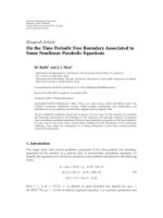
are alternating (see Figure 2.1).
Here Γ
ε
= Γ
ε
1
. Our first main result reads as follows.
Theorem 2.2. Suppose n
= 2.Foru ∈ H
1
(Ω,Γ
ε
1
), the following Friedrich’s inequality holds
true:

Ω
u
2
dx ≤ K
ε

Ω



∇
u


2
dx, K
ε
= K
0
+ ϕ(ε), (2.4)
where K
0
is a constant in Friedrich’s inequality (1.1) for functions u ∈
◦
H
1
(Ω),and
ϕ(ε)
∼(|lnε|)
−1/2
+(δ(ε)|lnε|)
1/2
as ε→0.
G. A. Chechkin et al. 3
δ
εδ
Figure 2.1. Plane domain.
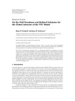
δ

εδ
Figure 2.2. Spatial domain.
For the case n ≥ 3, the geometr ical constructions are similar. We assume that ∂Ω =
S ∪ Γ, S ∩ Γ = ∅, Γ belongs to the hyperplane x
n
= 0, and Γ = Γ
ε
1
∪ Γ
ε
2
, Γ
ε
1
∩ Γ
ε
2
= ∅.
Denote by ω a bounded domain in the hyp erplane x
n
= 0, which contains the origin.
Without loss of generality ω
∈ ,where ={

x : −1/2 <x
i
< 1/2, i = 1, ,n − 1}, x =
(x,x
n
). Let ω

ε
be the domain {x : x/ε ∈ ω}. Denote by

Γ the integer translations of ω
ε
onthehyperplaneinx
i
direction, i = 1, ,n − 1. Finally, Γ
ε
1
={x : x/δ ∈

Γ}∩Γ, Γ
ε
2
=
Γ \ Γ
ε
1
(see Figure 2.2). In other words, Γ
ε
1
is a translations of vectors mδ(ε)e
i
(m ∈ Z, i =
1, ,n − 1) of a set diameter εδ(ε) contained in a ball of radius δ(ε). Here we assume that
δ(ε)
= o(ε
n−2
)asε→0. Also we suppose that Γ

ε
= Γ
ε
1
∪ S.
In this case our main result reads as follows.
Theorem 2.3. Suppose n
≥ 3.Foru ∈ H
1
(Ω,Γ
ε
1
∪ S), the following Friedrich’s inequality is
valid:

Ω
u
2
dx ≤ K
ε

Ω
|∇u|
2
dx, K
ε
= K
0
+ ϕ(ε), (2.5)
where K

0
is a constant in Friedrich’s inequality (1.1) for functions u ∈
◦
H
1
(Ω),and
ϕ(ε)
∼ε
n/2−1
+(δ(ε)ε
2−n
)
1/2
as ε→0.
4 Journal of Inequalities and Applications
Thus the precise dependence of the constant in Friedrich’s inequality of the small pa-
rameter ε will be established. Hence, it is possible to construct the lower and the upper
bounds for K
ε
.
3.Proofsofthemainresultsandsomeauxiliaryresults
In Sections 3.1 and 3.2 we discuss, present, and prove some auxiliary results, which are of
independent interest but also crucial for the proof of the main results in Section 3.3.
3.1. The relation between the constant in Friedrich’s inequality and the first eigenvalue
of a boundary value problem. Let Ω be some bounded domain w ith smooth bound-
ary ∂Ω, Γ
ε
⊂ ∂Ω. Suppose that the function u belongs to H
1
(Ω). Consider the following

problem:
Δu
=−λ
ε
u in Ω,
u
= 0onΓ
ε
,
∂u
∂ν
= 0on∂Ω \ Γ
ε
.
(3.1)
Definit ion 3.1. The function u
∈ H
1
(Ω,Γ
ε
) is a solution of problem (3.1), if the following
integral identity is valid:

Ω
∇u∇vdx= λ
ε

Ω
uv dx (3.2)
for all functions v

∈ H
1
(Ω,Γ
ε
).
The operator of problem (3.1) is positive and selfadjoint (it follows directly from the
integral identity). According to the general theory (see, e.g., [7]), all eigenvalues of the
problem are real, positive, and satisfy
0
≤ λ
1
ε
≤ λ
2
ε
≤···, λ
k
ε
−→ ∞ as k −→ ∞ . (3.3)
Here we assume that the eigenvalues λ
k
ε
are repeated according to their multiplicities.
Denote by μ
ε
the following value:
μ
ε
= inf
v∈H

1
(Ω,Γ
ε
)\{0}

Ω
|∇v|
2
dx

Ω
v
2
dx
. (3.4)
We need the following lemma (see the analogous lemma in [4]).
Lemma 3.2. The number μ
ε
is the first eigenvalue λ
1
ε
of the problem (3.1).
For the convenience of the reader we present the details of the proof.
Proof. It is sufficient to show that there exists such eigenfunction u
1
of problem (3.1),
corresponding to the first eigenvalue λ
1
ε
, that it satisfies

μ
ε
=

Ω


∇
u
1


2
dx

Ω

u
1

2
dx
. (3.5)
G. A. Chechkin et al. 5
Let
{v
(k)
} be a minimization sequence for (3.4), that is,
v
(k)

∈ H
1

Ω,Γ
ε

,


v
(k)


2
L
2
(Ω)
= 1,

Ω


∇
v
(k)


2
dx −→ μ
ε

,ask −→ ∞ .
(3.6)
It is obvious that the sequence
{v
(k)
} is bounded in H
1
(Ω,Γ
ε
). Hence, according to the
Rellich theorem, there exists a subsequence of
{v
(k)
}, converging weekly in H
1
(Ω,Γ
ε
)and
strongly in L
2
(Ω). For this subsequence, we keep the same notation {v
(k)
}.Wehavethat


v
(k)
− v
(l)



2
L
2
(Ω)
<η as k,l>k
0
(η). (3.7)
Using the following formula:




v
(k)
+ v
(l)
2




2
L
2
(Ω)
=
1
2



v
(k)


2
L
2
(Ω)
+
1
2


v
(l)


2
L
2
(Ω)
−




v
(k)
− v

(l)
2




2
L
2
(Ω)
, (3.8)
we obtain that




v
(k)
+ v
(l)
2




2
L
2
(Ω)
> 1 −

η
4
. (3.9)
From the definition of μ
ε
we conclude that

Ω
|∇v|
2
dx ≥ μ
ε
v
2
L
2
(Ω)
(3.10)
for all function v
∈ H
1
(Ω,Γ
ε
). Inequalities (3.9)and(3.10) give the following estimate:

Ω





∇

v
(k)
+ v
(l)
2





2
dx > μ
ε

1 −
η
4

. (3.11)
If k, l>k
0
(η), it follows that

Ω


∇
v

(k)


2
dx < μ
ε
+ η,

Ω


∇
v
(l)


2
dx < μ
ε
+ η. (3.12)
Hence,

Ω




∇

v

(k)
− v
(l)
2





2
dx
=
1
2

Ω


∇
v
(k)


2
dx +
1
2

Ω



∇
v
(l)


2
dx −

Ω




∇

v
(k)
+ v
(l)
2





2
dx
≤
μ

ε
+ η
2
+
μ
ε
+ η
2
− μ
ε

1 −
η
4

=
η

1+
μ
ε
4

−→
0, η −→ 0.
(3.13)
6 Journal of Inequalities and Applications
Finally, according to the Cauchy condition the sequence
{v
(k)

} convergestosomefunc-
tion v
∗
∈ H
1
(Ω,Γ
ε
) in the space H
1
(Ω,Γ
ε
), and

Ω


∇
v
∗


2
dx = μ
ε
,


v
∗



2
L
2
(Ω)
= 1. (3.14)
Assume that v
∈ H
1
(Ω,Γ
ε
) is an ar bitrary function. Denote
g(t)
=

Ω


∇

v
∗
+ tv



2
dx



v
∗
+ tv


2
L
2
(Ω)
. (3.15)
The function g(t)iscontinuouslydifferentiable in some neig hborhood of t
= 0. This ratio
has the minimum, which is equal to μ
ε
. Using the Fermat theorem, we obtain that
0
= g

|
t=0
=
2


v
∗


2
L

2
(Ω)

Ω

∇
v
∗
,∇v

dx − 2

Ω
v
∗
vdx

Ω


∇
v
∗


2
dx


v

∗


4
L
2
(Ω)
= 2

Ω

∇
v
∗
,∇v

dx − 2μ
ε

Ω
v
∗
vdx.
(3.16)
Thus, we have proved that

Ω

∇
v

∗
,∇v

dx = μ
ε

Ω
v
∗
vdx (3.17)
for v
∈ H
1
(Ω,Γ
ε
), that is, v
∗
satisfies the integral identity (3.1). This means that we have
found a function v
∗
such that

Ω


∇
v
∗



2
dx

Ω

v
∗

2
dx
= inf
v∈H
1
(Ω,Γ
ε
)\{0}

Ω


∇
v


2
dx

Ω
v
2

dx
= μ
ε
. (3.18)
Keeping in mind that u
1
= v
∗
we conclude that μ
ε
= λ
1
ε
. The proof is complete. 
Lemma 3.3. The following Friedrich inequality holds true:

Ω
U
2
dx ≤ K
ε

Ω
|∇U|
2
dx, U ∈ H
1

Ω,Γ
ε


, (3.19)
where K
ε
= 1/λ
1
ε
.
Proof. From Lemma 3.2 we get that
λ
1
ε
≤

Ω


∇
U


2
dx

Ω
U
2
dx
for any U
∈ H

1

Ω,Γ
ε

. (3.20)
Using this estimate, we deduce that

Ω
U
2
dx ≤
1
λ
1
ε

Ω
|∇U|
2
dx. (3.21)
Denoting by K
ε
the value 1/λ
1
ε
, we conclude the statement of our lemma. 
In the following section we will estimate λ
1
ε

.
G. A. Chechkin et al. 7
3.2. Auxiliary boundary v alue problems. Assume that f
∈ L
2
(Ω) and consider the fol-
lowing boundary value problems:
−Δu
ε
= f in Ω,
u
ε
= 0onΓ
ε
,
∂u
ε
∂ν
= 0onΓ
ε
2
,
(3.22)
−Δu
0
= f in Ω,
u
0
= 0on∂Ω.
(3.23)

Note that for n
= 2 we assume that Γ
ε
= Γ
ε
1
and for n ≥ 3 we assume that Γ
ε
= Γ
ε
1
∪ S.
Problem (3.23) is the homogenized (limit as ε
→0) problem for problem (3.22)(aproof
of this fact can be found in [4, 8], see also [6]).
Consider now the respective spectral problems:
−Δu
k
ε
= λ
k
ε
u
k
ε
in Ω,
u
k
ε
= 0onΓ

ε
,
∂u
k
ε
∂ν
= 0onΓ
ε
2
,
−Δu
k
0
= λ
k
0
u
k
0
in Ω,
u
k
0
= 0on∂Ω.
(3.24)
Next, let us estimate the difference
|1/λ
k
ε
− 1/λ

k
0
|. We will use the method introduced
by Ole
˘
ınik et al. (see [9, 10]).
Let H
ε
, H
0
be separable Hilbert spaces with the inner products (u
ε
,v
ε
)
H
ε
and (u,v)
H
0
,
and the norms
u
ε

H
ε
and u
H
0

, respectively; assume that ε is a small parameter, A
ε
∈
ᏸ(H
ε
), A
0
∈ ᏸ(H
0
) are linear continuous operators and ImA
0
⊂ V ⊂ H
0
,whereV is a
linear subspace of H
0
.
(C1) There exist linear continuous operators R
ε
: H
ε
→H
0
such that for all f ∈ V we
have (R
ε
f ,R
ε
f )
H

ε
→c( f , f )
H
0
as ε→0, where c = const > 0 does not depend on f.
(C2) The operators A
ε
, A
0
are positive, compact and selfadjoint in H
ε
, H
0
, respectively,
and sup
ε
A
ε

ᏸ(H
ε
)
< +∞.
(C3) For all f
∈ V we have A
ε
R
ε
f − R
ε

A
0
f 
H
ε
→0asε→0.
(C4) The sequence of operators A
ε
is uniformly compact in the following sense: if a se-
quence f
ε
∈ H
ε
is such that sup
ε
 f
ε

ᏸ(H
ε
)
< +∞, then there exist a subsequence
f
ε

and a vector w
0
∈ V such that A
ε


f
ε

− R
ε

w
0

H
ε

→0asε

→0.
Assume that the spectral problems for the operators A
ε
, A
0
are
A
ε
u
k
ε
= μ
k
ε
u
k

ε
, k = 1,2, , μ
1
ε
≥ μ
2
ε
≥···> 0,

u
l
ε
,u
m
ε

=
δ
lm
,
A
0
u
k
0
= μ
k
0
u
k

0
, k = 1,2, , μ
1
0
≥ μ
2
0
≥···> 0,

u
l
0
,u
m
0

=
δ
lm
,
(3.25)
8 Journal of Inequalities and Applications
where δ
lm
is the Kronecker symbol and the eigenvalues μ
k
ε
, μ
k
0

are repeated according to
their multiplicities.
The following theorem holds true (see [9]).
Theorem 3.4 (Ole
˘
ınik et al. [9, 10]). Suppose that the conditions (C1)–(C4)arevalid.
Then μ
k
ε
converges to μ
k
0
as ε→0, and the following estimate takes place:


μ
k
ε
− μ
k
0


≤
c
−1/2
sup
f ∈N(μ
k
0

,A
0
), f 
H
0
=1


A
ε
R
ε
f − R
ε
A
0
f


H
ε
, (3.26)
where N(μ
k
0
, A
0
) ={u ∈ H
0
, A

0
u = μ
k
0
u}. Assume also that k ≥ 1, s ≥ 1, are the integer
numbers, μ
k
0
= ··· = μ
k+s−1
0
and the multiplicity of μ
k
0
is equal to s. Then the re exist lin-
ear combinat ions U
ε
of the eigenfunctions u
k
ε
, ,u
k+s−1
ε
to problem (3.22) such that for all
w
∈ N(μ
k
0
, A
0

) we get U
ε
− R
ε
w
H
ε
→0 as ε→0.
To u se t he me th od of Ol e
˘
ınik et al. [9, 10], we define the spaces H
ε
and H
0
and the
operators A
ε
, A
0
,andR
ε
in an appropriate w ay.
Assume that H
ε
= H
0
= V = L
2
(Ω), and R
ε

is the identity operator. The operators A
ε
,
A
0
aredefinedinthefollowingway:A
ε
f = u
ε
, A
0
f = u
0
,whereu
ε
, u
0
are the solutions to
problems (3.22)and(3.23), respectively. Let us verify the conditions (C1)–(C4).
The condition (C1) is fulfilled automatically because R
ε
is the identity oper ator, c =
1. Let us verify the selfadjointness of the operator A
ε
. Define A
ε
f = u
ε
, A
ε

g = v
ε
, f ,g ∈
L
2
(Ω). Because of the integral identity of problem (3.22) the following identities are valid:

Ω
fv
ε
dx =

Ω
∇v
ε
∇u
ε
dx =

Ω
gu
ε
dx. (3.27)
Hence,

A
ε
f ,g

L

2
(Ω)
=

u
ε
,g

L
2
(Ω)
=

Ω
u
ε
gdx=

Ω
∇v
ε
∇u
ε
dx
=

Ω
fv
ε
dx =


f ,v
ε

L
2
(Ω)
=

f ,A
ε
g

L
2
(Ω)
.
(3.28)
The selfadjointness of the operator A
0
canbeprovedinananalogousway.
It is easy to prove the positiveness of the operator A
ε
:

A
ε
f , f

L

2
(Ω)
=

u
ε
, f

L
2
(Ω)
=

Ω
u
ε
fdx=

Ω


∇
u
ε


2
dx ≥ 0, (3.29)
and


Ω
|∇u
ε
|
2
dx > 0if f =0. The positiveness of A
0
may be proved in the same way.
Next, we prove that A
ε
, A
0
are compact operators: let the sequence { f
θ
} be bounded
in L
2
(Ω). It is evident that the sequence {A
ε
f
θ
}={u
ε,θ
} is bounded in H
1
(Ω,Γ
ε
) and the
sequence
{A

0
f
θ
}={u
0,θ
} is bounded in
◦
H
1
(Ω). Note that {u
ε,θ
} is bounded uniformly
on ε (for a proof see [4]). Because of compact embedding of the space H
1
(Ω)toL
2
(Ω),
we conclude that A
ε
and A
0
are compact operators. Moreover,


A
ε


ᏸ(H
ε

)
≤


u
ε


H
1
(Ω,Γ
ε
)
< ᏹ < +∞ (3.30)
G. A. Chechkin et al. 9
and, consequently,
sup
ε


A
ε


ᏸ(H
ε
)
< ᏹ < +∞. (3.31)
Let us verify the condition (C3). The operator R
ε

is the identity operator and, thus, it is
sufficient to prove that for all f
∈ L
2
(Ω)wehavethatA
ε
f − A
0
f 
L
2
(Ω)
→0asε→0, that is,
u
ε
− u
0

L
2
(Ω)
→0asε→0. It is enough to prove that u
ε
 u
0
in H
1
(Ω). (The week conver-
gence in H
1

(Ω) gives the strong convergence in L
2
(Ω).) The sequence u
ε
is uniformly
bounded in H
1
(Ω). Consequently, there exists a subsequence u
ε

,suchthatu
ε

 u
∗
in H
1
(Ω). Further we will set that u
ε
is the same subsequence. Let us show that
u
∗
≡ u
0
, that is, for all v ∈
◦
H
1
(Ω),


Ω
fvdx=

Ω
∇u
∗
∇vdx. (3.32)
The integral identity for problem (3.22) gives that

Ω
fvdx=

Ω
∇u
ε
∇vdx. (3.33)
Because u
∗
is a week limit of u
ε
in H
1
(Ω), the following is valid:

Ω
∇u
ε
∇vdx−→

Ω

∇u
∗
∇vdx when ε −→ 0 ∀v ∈ H
1
(Ω), (3.34)
and this gives us the desired result, because the integrals

Ω
∇u
∗
∇vdx and

Ω
fvdxdo
not depend on ε.
Let us verify the condition (C4). Consider the sequence
{ f
ε
}, which is bounded in
L
2
(Ω). Then A
ε
f
ε

H
1
(Ω,Γ
ε

)
=u
ε

H
1
(Ω,Γ
ε
)
≤ const, that is, the sequence {A
ε
f
ε
} is compact
in L
2
(Ω) and, consequently, there exists a subsequence ε

such that
A
ε

f
ε

−→ w
0
as ε

−→ 0, where w

0
∈ L
2
(Ω). (3.35)
Hence, we have that
A
ε

f
ε

− w
0

L
2
(Ω)
→0asε

→0.
Thus, the conditions (C1)–(C4) are valid.
It is evident that λ
k
ε
= 1/μ
k
ε
, λ
k
0

= 1/μ
k
0
. Using the estimate (3.26)wehave




1
λ
k
ε
−
1
λ
k
0




≤
sup
f ∈N(λ
k
0
,A
0
), f 
L

2
(Ω)
=1


A
ε
f − A
0
f


H
1
(Ω,Γ
ε
)
= sup
f ∈N(λ
k
0
,A
0
), f 
L
2
(Ω)
=1



u
ε
− u
0


H
1
(Ω,Γ
ε
)
,
(3.36)
where u
ε
, u
0
are the solutions of problems (3.22)and(3.23), respectively.
The following inequality was established in [4]:


u
ε
− u
0


H
1
(Ω,Γ

ε
)
≤ K f 
L
2
(Ω)


μ
ε

1/2
+

δ
μ
ε

1/2

, (3.37)
10 Journal of Inequalities and Applications
where μ
ε
= inf
u∈H
1
(Ω,Γ
ε
1

)\{0}
(

Ω
|∇u|
2
dx/

Ω
u
2
dx) and the constant K depends only on
the domain Ω. Moreover, the following asymptotics was proved in [4](thecasen
= 2)
and in [ 11](thecasen
≥ 3) (see also [8, 12]):
μ
ε
=
⎧
⎪
⎪
⎪
⎨
⎪
⎪
⎪
⎩
π
|lnε|

+ O

1
|lnε|
2

,ifn = 2,
ε
n−2
σ
n
2
c
ω
+ O

ε
n−1

,ifn>2,
(3.38)
as ε
→0.
Here σ
n
is the area of the unit sphere in R
n
,andc
ω
> 0 is the capacity of the (n − 1)-

dimensional “disk” ω (see [13, 14]).
Define the following value:
ϕ(ε)
≡ K


μ
ε

1/2
+

δ
μ
ε

1/2

. (3.39)
Note that if n
= 2, it implies that μ
ε
∼1/|lnε| and δ = O(1/|lnε|). Consequently, we
have
δ
μ
ε
=
o


1/|lnε|

|lnε|
π
= o(1) (3.40)
as ε
→0.
Inthesameway,ifn>2 it yields that
δ
μ
ε
∼o(1) (3.41)
as ε
→0.
Using this asymptotics, we deduce
ϕ(ε)
= K
⎧
⎪
⎨
⎪
⎩
(lnε)
−1/2
+

δ(ε)|lnε|

1/2
+ o


(lnε)
−1/2
+

δ(ε)|lnε|

1/2

,ifn = 2,
ε
n/2−1
+

δ(ε)ε
n−2

1/2
+ o

ε
n/2−1
+

δ(ε)ε
n−2

1/2

,ifn>2,

(3.42)
as ε
→0.
Finally, due to (3.36), (3.37), and (3.38)wegetthat




1
λ
1
ε
−
1
λ
1
0




≤
ϕ(ε), (3.43)
where ϕ(ε)hastheasymptotics(3.42).
3.3. Proofs of the main results.
Proof of Theorem 2.2. Actually, because of estimate (3.19), Friedrich’s inequality

Ω
u
2

dx ≤
1
λ
1
ε

Ω
|∇u|
2
dx, u ∈ H
1

Ω,Γ
ε

(3.44)
G. A. Chechkin et al. 11
is valid. The estimate (3.43) implies that
1
λ
1
ε
≤
1
λ
1
0
+ ϕ(ε). (3.45)
By rewriting inequality (3.44), using the established relations between λ
1

ε
and λ
1
0
we
find that

Ω
u
2
dx ≤
1
λ
1
ε

Ω
|∇u|
2
dx ≤

1
λ
1
0
+ ϕ(ε)


Ω
|∇u|

2
dx. (3.46)
According to our notations, 1/λ
1
0
= K
0
. Thus, for u ∈ H
1
(Ω,Γ
ε
), the following Friedrich
inequality holds true:

Ω
u
2
dx ≤ K
ε

Ω
|∇u|
2
dx, K
ε
= K
0
+ ϕ(ε), (3.47)
where ϕ(ε)
∼(|lnε|)

−1/2
+(δ(ε)|lnε|)
1/2
as ε→0, if n = 2. Hence, the proof is complete.

Proof of Theorem 2.3. The proof is completely analogous to that of Theorem 2.2: using
inequalities (3.19), (3.42), and (3.43), we obtain the asymptotics of the constant K
ε
,hence
weleaveoutthedetails.Noteonlythatinthiscaseϕ(ε)
∼ε
n/2−1
+(δ(ε)ε
n−2
)
1/2
as ε→0.

4. Special cases
In this section, we consider domains with special geometry.
Let ∂G be the boundar y of the unit disk G centered at the origin. Assume that ω
ε
=
{
(r,θ):r = 1, −δ(ε)(π/2) <θ<δ(ε)(π/2)} is the a rc, where (r,θ) are the polar coordi-
nates. Suppose also that η
ε
= (−εδ,εδ). Denote γ
ε
= ∂G \ Γ

ε
,whereΓ
ε
is the union of the
sets obtained from η
ε
by rotation about the origin through the angle επ and its multi-
ples. For simplicity we assume here that ε
= 2/N, N ∈ N.Letᏼ be an arbitrary conformal
mapping of a disk with radius exceeding 1, let Ω be the image of the unit disk G and let
Γ
ε
1
= ᏼ(Γ
ε
), Γ
ε
2
= ᏼ(γ
ε
).
For this domain we have the following theorem (see [15–17]).
Theorem 4.1. Suppose that n
= 2, the domain Ω istheimageoftheunitdiskG as defined at
the beginning of the section and δ lnε
→0 as ε→0.Foru ∈ H
1
(Ω,Γ
ε
1

), the following Friedrich
inequality holds true:

Ω
u
2
dx ≤ K
ε

Ω
|∇u|
2
dx, K
ε
= K
0
+ ϕ(ε), (4.1)
where K
0
is a c onstant in Friedrich’s inequality (1.1) for functions u ∈
◦
H
1
(Ω),andϕ(ε) =
δ lnsinε

∂Ω
(∂ψ
0
/∂ν)

2
|Ᏺ

|ds+ o(δ) as ε→0, where ψ
0
is the firs t normalized in L
2
(Ω) eigen-
function of the problem
−Δψ
0
= K
0
ψ
0
, x ∈ Ω; ψ
0
= 0, x ∈ ∂Ω, (4.2)
and Ᏺ
= ᏼ
−1
.
12 Journal of Inequalities and Applications
If the mapping ᏼ is identical, then the following statement takes place (see [15–18]).
Theorem 4.2. Suppose that n = 2, the domain Ω is the unit disk and δ lnε→0 as ε→0.For
u
∈ H
1
(Ω,Γ
ε

1
), the following Friedrich inequality holds true:

Ω
u
2
dx ≤ K
ε

Ω
|∇u|
2
dx,
K
ε
= K
0

1+2δ lnsinε +2δ
2
(lnsinε)
2
+ o

δ
2

(4.3)
as ε
→0,whereK

0
is a constant in Friedrich’s inequality (1.1) for functions u ∈
◦
H
1
(Ω).
Note that nonperiodic geometry are considered in [19]. In the paper the author con-
structed and verified the asymptotic expansions of eigenvalues. Keeping in mind these
results it is possible to obtain sharp bounds for the constant in Friedrich’s inequalit y.
Acknowledgments
The research presented in this paper was initiated at a research stay of G. A. Chechkin at
Lule
˚
a University of Technolog y, Lule
˚
a, Sweden, in June 2005. The final version was com-
pleted when G. A. Chechkin was visiting Laboratoire J L. Lions de l’Universit
´
ePierreet
Marie Curie, Paris, France, in March-April 2007. The authors thank the referees for sev-
eral valuable comments and suggestions, which have improved the final version of the
paper. The work of the first author was partially supported by RFBR (06-01-00138). The
work of the first and the second authors was partially supported by the program “Lead-
ing Scientific Schools” (HIII-1698.2008.1). The work of the second author was partially
supported by RFBR.
References
[1] A. Kufner and L E. Persson, Weighted Inequalities of Hardy Type, World Scientific, River Edge,
NJ, USA, 2003.
[2] A. Kufner, L. Maligranda, and L E. Persson, The Hardy Inequality. About Its History and Related
Results, Vydavetelsky Servis, Pilsen, Germany, 2007.

[3] B. Opic and A. Kufner, Hardy-Type Inequalities, vol. 219 of Pitman Research Notes in Mathematics
Series, Longman Scientific & Technical, Harlow, UK, 1990.
[4] G. A. Chechkin, “Averaging of boundary value problems with singular perturbation of the
boundary conditions,” Russian Academy of Sciences. Sbornik. Mathematics,vol.79,no.1,pp.
191–222, 1994, translation in Matematicheski
˘
ı Sbornik, vol. 184, no. 6, pp. 99–150, 1993.
[5] V. G. Maz’ya, Prostranstva S. L. Soboleva, Leningrad University, Leningrad, Russia, 1985.
[6] G. A. Chechkin, A. L. Piatnitski, and A. S. Shamaev, Homogenization: Methods and Applications,
vol. 234 of Translations of Mathematical Monographs, American Mathematical Society, Provi-
dence, RI, USA, 2007.
[7] V. S. Vladimirov, The Equations of Mathematical Physics, Nauka, Moscow, Russia, 3rd edition,
1976.
[8] G. A. Chechkin, “On the estimation of solutions of boundary-value problems in domains with
concentrated masses periodically distributed along the boundary. The case of “light” masses,”
Mathematical Notes, vol. 76, no. 6, pp. 865–879, 2004, translation in Matematicheskie Zametki,
vol. 76, no. 6, pp. 928–944, 2004.
G. A. Chechkin et al. 13
[9] O. A. Ole
˘
ınik, A . S. Shamaev, and G. A. Yosifian, Mathematical Problems in Elasticity and Homog-
enization, vol. 26 of Studies in Mathematics and Its Applications, North-Holland, Amsterdam,
The Netherlands, 1992.
[10] G. A. Iosif’yan, O. A. Ole
˘
ınik, and A. S. Shamaev, “On the limit behavior of the spectrum of a
sequence of operators defined in different Hilbert spaces,” Russian Mathematical Surveys, vol. 44,
no. 3, pp. 195–196, 1989, translation in Uspekhi Matematicheskikh Nauk, vol. 44, no. 3(267), pp.
157–158, 1989.
[11] R. R. Gadyl’shin and G. A. Chechkin, “A boundary value problem for the Laplacian with rapidly

changing type of boundary conditions in a multi-dimensional domain,” Siberian Mathematical
Journal, vol. 40, no. 2, pp. 229–244, 1999, translation in Sibirski
˘
ı Matematicheski
˘
ıZhurnal, vol.
40, no. 2, pp. 271–287, 1999.
[12] A. G. Belyaev, G. A. Chechkin, and R. R. Gadyl’shin, “Effective membrane permeability: esti-
mates and low concentration asymptotics,” SIAM Journal on Applied Mathematics,vol.60,no.1,
pp. 84–108, 2000.
[13] N. S. Landkof, Foundations of Modern Potential Theory, Springer, New York, NY, USA, 1972.
[14] G. P
´
olya and G. Szeg
¨
o, Isoperimetric Inequalities in Mathematical Physics, Annals of Mathematics
Studies, no. 27, Princeton University Press, Princeton, NJ, USA, 1951.
[15] R. R. Gadyl’shin, “On the asymptotics of eigenvalues for a per iodically fixed membrane,” St.
Petersburg Mathematical Journal, vol. 10, no. 1, pp. 1–14, 1999, translation in Algebra I Analiz,
vol. 10, no. 1, pp. 3–19, 1998.
[16] R. R. Gadyl’shin, “A boundary value problem for the Laplacian with rapidly oscillating bound-
ary conditions,” Doklady Mathematics, vol. 58, no. 2, pp. 293–296, 1998, translation in Doklady
Akademii Nauk, vol. 362, no. 4, pp. 456–459, 1998.
[17] D. I. Borisov, “Two-parametrical asymptotics for the eigenevalues of the laplacian with frequent
alternation of boundary conditions,” Journal of Young Scientists. Applied Mathematics and Me-
chanics, vol. 1, pp. 36–52, 2002 (Russian).
[18] D. I. Borisov, “Two-parameter asymptotics in a boundary value problem for the Laplacian,”
Mathematical Notes, vol. 70, no. 3-4, pp. 471–485, 2001, translation in Matematicheskie Zametki,
vol. 70, no. 4, pp. 520–534, 2001.
[19] D. I. Borisov, “Asymptotics and estimates for the eigenelements of the Laplacian with frequent

nonperiod change of boundary conditions,” Izvestiya. Seriya Matematicheskaya, vol. 67, no. 6,
pp. 1101–1148, 2003, translation in Izvestiya Rossiiskoi Akademii Nauk. Seriya Matematich-
eskaya, vol. 67, no. 6, pp. 23–70, 2003.
G. A. Chechkin: Department of Differential Equations, Faculty of Mechanics and Mathematics,
Moscow Lomonosov State University, Moscow 119991, Russia
Email address:
Yu.O.Koroleva:DepartmentofDifferential Equations, Faculty of Mechanics and Mathematics,
Moscow Lomonosov State University, Moscow 119991, Russia
Email address:
L E. Persson: Department of Mathematics, Lule
˚
a University of Technology, 97187 Lule
˚
a, Sweden
Email address: