Báo cáo hóa học: " Research Article Design and Performance Analysis of an Adaptive Receiver for Multicarrier DS-CDMA" doc

Hindawi Publishing Corporation
EURASIP Journal on Wireless Communications and Networking
Volume 2007, Article ID 10462, 10 pages
doi:10.1155/2007/10462
Research Article
Design and Performance Analysis of an Adaptive Receiver for
Multicarrier DS-CDMA
Huahui Wang, Kai Yen, Kay Wee Ang, and Yong Huat Chew
Institute for Infocomm Research (I
2
R) (A
∗
STAR), Agency for Science, Technology and Research,
21 Heng Mui Keng Terrace, Singapore 119613
Received 26 January 2006; Revised 22 Januar y 2007; Accepted 21 May 2007
Recommended by Lee Swindlehurst
An adaptive parallel interference cancelation (APIC) scheme is proposed for the multicarrier direct sequence code division multiple
access (MC-DS-CDMA) system. Frequency diversity inherent in the MC system is exploited through maximal ratio combining,
and an adaptive least mean square algorithm is used to estimate the multiple access interference. Theoretical analysis on the bit-
error rate (BER) of the APIC receiver is presented. Under a unified signal model, the conventional PIC (CPIC) is shown to be a
special case of the APIC. Hence the BER derivation for the APIC is also applicable to the CPIC. The performance and the accuracy
of the theoretical results are examined via simulations under different design parameters, which show that the APIC outperforms
the CPIC receiver provided that the adaptive parameters are properly selected.
Copyright © 2007 Huahui Wang et al. This is an open access article distributed under the Creative Commons Attribution License,
which permits unrestricted use, distribution, and reproduction in any medium, provided the original work is properly cited.
1. INTRODUCTION
Future generations of broadband wireless mobile communi-
cation systems are expected to support various services over
a multitude of channels encountered in indoor, open rural,
suburban, and urban environments, while maintaining the
required quality of service (QoS) [1, 2]. In order to meet

these demands, the signal should be flexibly designed such
that it is capable of adapting to these communication condi-
tions. In the existing direct-sequence code-division multiple
access (DS-CDMA) systems, the spread spectrum (SS) mod-
ulation is exploited in mitigating various problems encoun-
tered in different communication media. Recently, the multi-
carrier (MC) technique has become an important alternative
for achieving this goal [3, 4].
A number of MC-CDMA schemes have been proposed
in the literature [5–9]. Their performances are analyzed and
compared with that of single carrier (SC) DS-CDMA systems
in frequency-selective Rayleigh fading channels [9–13]. MC
systems are advantageous due to their robustness in com-
bating the frequency selectiv ity in broadband channels. The
underlying reason is the integration of an orthogonal fre-
quency division multiplexing (OFDM) overlay, which can be
designed such that each subcarrier undergoes flat fading and
hence reduces the severe intersymbol interference (ISI) en-
countered in SC-DS-CDMA systems.
On the other hand, the critical issue for MC-CDMA sys-
tems remains to be the improvement of the system capacity
in multiuser communications, in which the multiple access
interference (MAI) becomes the major capacity-limiting fac-
tor. Much attention has been given to the per formance anal-
ysis of the MC systems based on the single user detection
(SUD) strategy, see [4, 14, 15], for example, where the MAI is
simply treated as thermal noise. Significant improvement can
be achieved when multiuser detection (MUD) techniques are
employed to jointly detect all the users’ signals [16, 17]. Most
MUD algorithms originally proposed for SC-DS-CDMA are

applicable to MC-CDMA systems, where interest in this area
has been mainly focused on the performance analysis of these
various techniques.
It is well known that the prohibitive complexity of the
optimal multiuser detection necessitates suboptimal solu-
tions having lower complexity. A large volume of subopti-
mal MUD algorithms have been proposed in the literature,
and two different approaches emerge, namely, adaptive filter-
ing [18–20] and interference cancelation (IC) [21–23]. Much
more research has been dedicated to the latter primarily due
to a simpler analysis tractability. There are two main varieties
of IC schemes, namely, serial IC (SIC) and parallel IC (PIC).
In SIC, MAI is estimated and subtracted from the received
signal sequentially. Adaptation of SIC to MC systems can be
foundin[21, 22], where the system performances are also
2 EURASIP Journal on Wireless Communications and Networking
Serial to parallel conv erter
Parallel-
bit branch
.
.
.
d
(k)
P
d
(k)
1
1
2

.
.
.
M
1
2
.
.
.
M
c
(k)
(t)
c
(k)
(t)
c
(k)
(t)
c
(k)
(t)
c
(k)
(t)
c
(k)
(t)
cos(ω
1,1

t + ϕ
1,1
)
cos(ω
1,2
t + ϕ
1,2
)
.
.
.
cos(ω
1,M
t + ϕ
1,M
)
.
.
.
cos(ω
P,1
t + ϕ
P,1
)
.
.
.
cos(ω
P,2
t + ϕ

P,2
)
Identical-bit
stream
cos(ω
P,M
t + ϕ
P,M
)
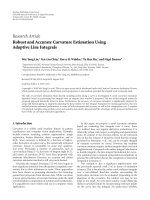
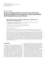
Figure 1: Illustration of signal transmission for user k.
analyzed. PIC appears to be more attractive in the case when
high speed detection is preferred, since the cancelation of the
interference is performed in parallel. However, the potential
gain from PIC depends on the precise estimate of the MAI. A
partial PIC is proposed in [24] to mitigate the effect of unre-
liable MAI estimation. Motivated by [24], a hybrid approach
comprising of the PIC and an adaptive technique is proposed
for SC-DS-CDMA in [25].
In this paper, an adaptive parallel interference cancela-
tion (APIC) scheme is proposed for the MC-DS-CDMA sys-
tem, in which the frequency diversity inherent in the MC sys-
tem is exploited through maximal ratio combining (MRC).
The contribution of the paper is twofold. Firstly, the adap-
tive signal processing as well as the IC technique is designed
for the MC system, and the conditions under which the al-
gorithms are able to function properly are investigated. Sec-
ondly, instead of simply implementing a heuristic algorithm,
we perform a thorough analysis on the system performance
and obtain a simple closed form expression for the bit-error
rate (BER) of the APIC receiver. Furthermore, under the uni-

fied signal model, we show that the theoretical result de-
rived for the APIC is also applicable to the conventional PIC
(CPIC), as long as the adaptive step-size is set to zero. The ac-
curacy of the BER derivation is validated by computer sim-
ulations. The results showed a significant performance im-
provement of the APIC over the CPIC receiver.
The organization of this paper is as follows. Section 2 in-
troduces the MC-DS-CDMA system model. Section 3 high-
lights the structure of the APIC receiver with pre- and
post-MRC combining. Section 4 analyzes the performance of
the receiver and derives the corresponding closed form BER
expression. Numerical results and discussions are presented
in Section 5. We conclude the paper in Section 6 .
2. SYSTEM MODEL
The structure of the transmitter for user k is shown in
Figure 1.AblockofP incoming bits is first serial-to-parallel
converted into P so-called parallel-bit branches. The bit on
each parallel-bit branch, denoted as d
(k)
p
, p = 1, 2, , P,is
then replicated into M streams referred to as identical-bit
streams, as shown in Figure 1. These M
× P bit streams are
spread by the same user-specific pseudorandom spreading
sequence c
(k)
(t), and modulated on subcarriers that are or-
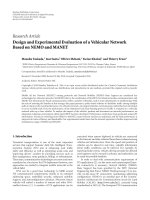
thogonal to each other. In order to ensure independent fad-
ing and hence achieving frequency diversity, the M

× P sub-
carriers are assigned in such a way that the frequency separa-
tion between all identical-bit subcarriers is maximized, as il-
lustrated in Figure 2, where the identical-bit subcarriers f
p,m
,
m
= 1, 2, , M, corresponding to data d
(k)
p
are separated by
a distance of P/T
c
for two neighboring subcarriers, for exam-
ple, f
p,m
and f
p,m+1
.
In this paper, the channel is assumed to be a slow-
varying, frequency-selective Rayleigh fading channel with a
delay spread of T
m
. Since the spread spectrum system can
resolve multipath signals with delay larger than one chip
duration, for an SC-DS-CDMA system with a chip duration
of T

c
, the number of resolvable paths L


is given by
L

=

T
m
/T

c

+1, (1)
Huahui Wang et al. 3
2/T
c
f
1,1
···
f
P,1
f
1,2
···
f
1,m
···
f
P,m
···

f
1,M
···
f
P,M
··· ··· ··· · ·· · ··
(MP +1)/T
c
Figure 2: Spectrum of the tr ansmitted signal.
where x is themaximum integer less than or equal to x.As-
suming a passband null-to-null bandwidth, the transmission
bandwidth for the SC-DS-CDMA is 2/T

c
. Maintaining this
bandwidth, if the chip duration on each subcarrier of the
MC-DS-CDMA system is T
c
, then the following condition
shouldbesatisfied(refertoFigure 2):
2
T

c
=
MP +1
T
c
. (2)
From (1)and(2), the number of resolvable paths L on each

subcarrier of the MC-DS-CDMA system is L
=T
m
/T
c
+1 =

2(L

− 1)/(MP +1) + 1. It is easy to show that when P and
M are chosen to satisfy [4]
MP
≥ 2(L

− 1), (3)
then L
= 1 and each subcarrier experiences a flat fading
channel. In this case, the complex channel gain for the qth
subcarrier of user k can be defined as
ζ
(k)
q
(t) = α
(k)
q
(t)exp

jβ
(k)
q

(t)

,(4)
where α
(k)
q
(t) is a Rayleigh-distributed stochastic process with
unit second moment and β
(k)
q
(t) is uniformly distributed
over 0 and 2π. It is assumed that the channel gain ζ
(k)
q
(t)
is independent and identically distributed (i.i.d.) for differ -
ent values of k and q. This is a slight simplification over
a real channel which would be correlated in frequency, but
typically the difference in performance between a correlated
and uncorrelated channel model is small, except that the
correlation is noticeable [21 , 26]. Furthermore, we investi-
gate synchronous MC-DS-CDMA systems with BPSK mod-
ulation to considerably simplify the exposition and analysis.
Synchronous systems are becoming more of practical inter-
est since quasisynchronous approach has been proposed for
satellite and microcell applications [27]. In [28], an uplink
synchronous CDMA system is investigated, where users’ sig-
nals are assumed aligned at the base station. In this paper, we
consider a similar uplink synchronous MC-DS-CDMA sys-
tem and study its performance.

Assuming that the system consists of K number of users
and that all the users employ the same transmitter structure
of Figure 1, the received signal at the base station can be writ-
ten as
r(t)
=
K

k=1
P

p=1
M

m=1

2P
k
M
d
(k)
p
p
T
b

t − T
b

c

(k)
(t)
× ζ
(k)
q
(t)cos

ω
q
t + φ
q

+ n(t),
(5)
where P
k
is the power of the kth user, d
(k)
p
∈{−1, +1} is the
kth user’s pth parallel-bit data, T
b
is the transmission inter-
val for each block of data, p
τ
(t) is defined as the rectangular
pulse waveform with unit amplitude and duration τ, ω
q
and
φ

q
are the frequency and random phase of the qth subcarrier,
respectively, and c
(k)
(t) is the spreading sequence of user k,
which is g iven by
c
(k)
(t) =
∞

n=−∞
c
(k)
(n)p
T
c

t − nT
c

,(6)
where c
(k)
(n) is the nth chip of the long spreading sequence
for user k. Suppose each symbol interval contains N chips,
we conduct normalization in each symbol period such that

(l+1)N−1
n

=lN
[c
(k)
(n)]
2
= 1, l ∈ Z. N is called the processing
gain. Since we have assumed that the channel is slowly fading,
the channel gain ζ
(k)
q
(t) will remain constant for one trans-
mission interval. Hence the function of time in ζ
(k)
q
(t)will
be omitted hereafter. The parameter q
= p +(m − 1)P is the
subcarrier index corresponding to the pth parallel-bit branch
and the mth identical-bit stream. The variable n(t)in(5)is
the additive white Gaussian noise (AWGN) with zero mean
and one-sided power spectral density of N
0
.
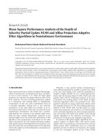
3. ADAPTIVE RECEIVER STRUCTURE
The structure of the proposed adaptive receiver is illustrated
in Figure 3, which can be functionally divided into three
parts: the pre- and post-MRC combining, the adaptive MAI
estimation, and the parallel IC.
3.1. Initial stage: MF with MRC (MF-MRC)
Referring to Figure 3, after the received signal is down con-

verted to its equivalent baseband signal and passed through
the fast Fourier tr ansform (FFT) block, the signal can be
grouped into P sets, where each set consists of M identical-
bit streams. For description simplicity, we only consider the
processing of the pth branch in the sequel. For the qth sub-
carrier where q
= p+(m−1)P, the coherently detected signal
corresponding to the nth chip, r
q
(n), is given by
r
q
(n) =

(n+1)T
c
nT
c
r(t)cos

ω
q
t + φ
q

dt
=
K

k=1

v
(k)
q
(n)+η
t
(n), 0 ≤ n ≤ N − 1,
(7)
where
v
(k)
q
(n) =

P
k
2M
d
(k)
p
c
(k)
(n)ζ
(k)
q
,(8)
η
t
(n) =

(n+1)T

c
nT
c
n(t)cos

ω
q
t + φ
q

dt. (9)
It is easy to show that η
t
(n) is a zero mean Gaussian random
variable with variance σ
2
η
= N
0
/2.
4 EURASIP Journal on Wireless Communications and Networking
r(t)
FFT
r
P,M
.
.
.
r
P,1

r
p,M
.
.
.
.
.
.
r
p,1
.
.
.
r
1,M
.
.
.
r
1,1
MF
MF
u
(K)
p,M
.
.
.
u
(1)

p,M
.
.
.
u
(K)
p,1
.
.
.
u
(1)
p,1
MRC
MRC

d
(1)
p

d
(K)
p
Pre-combining
Signal
reconstruction
Signal
reconstruction
Reference signal
Reference signal

MAI reconstruction
s
(K)
p,M
.
.
.
s
(K)
p,1
.
.
.
s
(1)
p,M
.
.
.
s
(1)
p,1
.
.
.
.
.
.
Weights
adjustment

MAI
estimate
Weights
adjustment
MAI
estimate
w
(K)
p,M
.
.
.
w
(1)
p,M
.
.
.
w
(K)
p,1
w
(1)
p,1
.
.
.
PIC stage
.
.

.
.
.
.
PIC
PIC
x
(K)
p,M
.
.
.
x
(1)
p,M
x
(K)
p,1
x
(1)
p,1
.
.
.
Postcombining
MF
MF
.
.
.

.
.
.
.
.
.
.
.
.
MRC
.
.
.
MRC

d
(K)
p

d
(1)
p
Figure 3: Adaptive receiver design.
The signal r
q
(n) is then passed to the chip-rate matched
filter (MF) bank, as depicted in Figure 3.Theoutputcorre-
sponding to the nth chip of the kth user is g iven by
u
(k)

q
(n) = r
q
(n)c
(k)
(n), 0 ≤ n ≤ N − 1. (10)
Assuming perfect channel estimation, the M outputs corre-
sponding to the identical-bit streams are combined together
using the MRC coefficients g
(k)
q
= [ζ
(k)
q
]
∗
, where [x]
∗
is the
complex conjugate of x. If the user of interest is user 1, the
tentative decision

d
(1)
p
is then given by

d
(1)
p

= sign



N−1

n=0
M

m=1
u
(1)
q
(n)g
(1)
q

. (11)
3.2. MAI estimation stage
After the initial decision

d
(k)
p
is obtained, it is replicated into
M branches to reconstruct the MAI, as shown in Figure 3.
Similar to the transmitter, each of the M copiesisspreadby
the corresponding user’s spreading code c
(k)
(n)andattenu-

ated by the channel gain ζ
(k)
q
. Hence the regenerated signal of
the nth chip corresponding to the qth carrier is given by
s
(k)
q
(n) =

P
k
2M

d
(k)
p
c
(k)
(n)ζ
(k)
q
,1≤ m ≤ M. (12)
The regenerated signals of all the users are multiplied by
their corresponding adaptive weights w
(k)
q
(n) and summed
together to produce an estimate
r

q
(n) of the signal r
q
(n),
which is written as
r
q
(n) =
K

k=1
s
(k)
q
(n)w
(k)
q
(n), 0 ≤ n ≤ N − 1. (13)
The difference between r
q
(n)andr
q
(n) constitutes the MAI
estimation error. Based on this error we define the cost func-
tion of the adaptive algorithm as
ε
q
= E




e
q
(n)


2

=
E



r
q
(n) − r
q
(n)


2

, (14)
where E[
·] is the statistical expectation operator and e
q
(n) =
r
q
(n) − r

q
(n) is the error of the MAI estimation. In order
to minimize the cost, the weights w
(k)
q
(n) are adjusted at the
chip rate according to the normalized LMS algorithm [29]:
w
(k)
q
(n +1)= w
(k)
q
(n)+
μ
· s
(k)
q
(n)

K
i=1

s
(i)
q
(n)

2


e
q
(n)

∗
, (15)
where μ denotes the step-size. At the end of one transmission
interval, the weight w
(k)
q
(N − 1) is determined and it is used
by the next stage to assist in the interference cancelation, as
depicted in Figure 3.
3.3. Cancelation with MRC stage: PIC-MRC
At this stage, w
(k)
q
(N − 1) is used to weight the input signal
s
(k)
q
(n) over the entire transmission interval. Subtracting the
weighted MAI, the “cleaner” signal for user 1 is given by
x
(1)
q
(n) = r
q
(n) −
K


k=2
v
(k)
q
(n), (16)
where
v
(k)
q
(n) = s
(k)
q
(n)w
(k)
q
(N − 1). (17)
The signal x
(1)
q
(n) is then passed to the MF bank and the M
identical-bit streams are combined via MRC. The final deci-
sion is then obtained according to

d
(1)
p
= sign




N−1

n=0
M

m=1
x
(1)
q
(n)c
(1)
(n)g
(1)
q

. (18)
Huahui Wang et al. 5
A multistage APIC receiver can be realized by repeating the
process from (12)to(18).
4. PERFORMANCE ANALYSIS
4.1. BER of the MF-MRC receiver
In Figure 3, if we only consider the first stage, then the
structure becomes a conventional MF with MRC combining,
which we will refer to as the MF-MRC receiver in the follow-
ing context. The soft output of the MF-MRC receiver for user
1isgivenby
Z
(1)
= D + n

t
+ I
MAI
, (19)
where u
(1)
q
(n)wasdefinedin(10). The desired signal D is
given by
D
=
M

m=1
N
−1

n=0
v
(1)
q
(n)c
(1)
(n)

ζ
(1)
q

∗

=

P
1
2M
d
(1)
p
M

m=1

α
(1)
q

2
,
(20)
and the noise term n
t
is given by
n
t
=

M

m=1
N

−1

n=0
η
t
(n)c
(1)
(n)α
(1)
q
exp

−
jβ
(1)
q


. (21)
n
t
is a zero mean Gaussian random variable and its variance
is given by
σ
2
n
=
N
0
4

M

m=1

α
(1)
q

2
. (22)
The term I
MAI
in (19) is the MAI which can be written into
two parts:
I
MAI
= I
(s)
MAI
+ I
(d)
MAI
, (23)
where I
(d)
MAI
is the interference from the other users on differ-
ent subcarriers, which simply vanishes in synchronous case
[4]. I
(s)

MAI
is the interference from the other users on the same
subcarrier, which is given by
I
(s)
MAI
=

M

m=1

T
b
0
K

k=2

2P
k
M
d
(k)
p
p
T
b

t − T

b

c
(k)
(t)
× ζ
(k)
q
cos

ω
q
t+φ
q

c
(1)
(t)cos

ω
q
t+φ
q

ζ
(1)
q

∗
dt


=
M

m=1
K

k=2
N
−1

n=0

P
k
2M
d
(k)
p
c
(k)
(n)c
(1)
(n)
× cos

β
(k)
q
− β

(1)
q

α
(k)
q
α
(1)
q
.
(24)
The term I
(s)
MAI
is commonly approximated as a zero mean
Gaussian r andom variable. Under the assumption that α
(1)
q
is known at the receiver and the channel is normalized with
E[(α
(k)
q
)
2
] = 1, the variance of I
(s)
MAI
is given by
Var


I
(s)
MAI

=
K

k=2
P
k
4MN
M

m=1

α
(1)
q

2
. (25)
Let γ
=

M
m=1
[α
(1)
q
]

2
, and assuming that a bit “1” is trans-
mitted, then the error probability conditioned on γ is given
by
P[e
| γ] =
1
2
erfc

E

Z
(1)


2Var

Z
(1)


=
1
2
erfc


P
1

/(2M)γ

2

Var

I
MAI

+ σ
2
n


.
(26)
Assuming that any bit can be sent via any of the P parallel
branches with equal probability, the final BER of the MF-
MRC receiver (the initial stage of the APIC receiver) can be
written as
P
ini
[e] =
1
P
P

p=1

∞

0
P

e | γ

p(γ)dγ, (27)
where p(γ) is the probability density function of γ and is
given by [30]
p(γ)
=
1
(M − 1)
γ
M−1
e
−γ
. (28)
4.2. BER of the conventional PIC receiver
In Figure 3, when there is no adaptive process involved, or
equivalently by setting the weight w
(k)
q
(N −1) = 1 in the MAI
estimation stage, the receiver reduces to a conventional PIC
receiver (CPIC). For CPIC, the IC is performed by subtract-
ing the estimated signals of the interfering users from the ref-
erence signal r
q
(n), which forms a “cleaner” signal x
(1)

q
(n)as
given by
x
(1)
q
(n) = r
q
(n) −
K

k=2
s
(k)
q
(n), (29)
where s
(k)
q
(n) is the regenerated signal defined in (12). The
output signal after the MRC combining is given by

Z
(1)
=

M

m=1
N

−1

n=0
x
(1)
q
(n)c
(1)
(n)

ζ
(1)
q

∗

=
D + n
t
+ I

MAI
.
(30)
The desired signal D and the noise term n
t
above are identical
with the corresponding terms in (20)and(21). The new MAI
term is given by
I


MAI
=
M

m=1
K

k=2
N
−1

n=0

P
k
2M

d
(k)
p
−

d
(k)
p

c
(k)
(n)

× c
(1)
(n)cos

β
(k)
q
− β
(1)
q

α
(k)
q
α
(1)
q
.
(31)
6 EURASIP Journal on Wireless Communications and Networking
If the BER of the initial stage, P
ini
[e], is available, then we
have [31]
P


d
(k)
p

=−d
(k)
p
| d
(k)
p

=
P
ini
[e],
P


d
(k)
p
= d
(k)
p
| d
(k)
p

=
1 − P
ini
[e],
(32)
E


d
(k)
p
−

d
(k)
p

2

=
4P
ini
[e]. (33)
From (25)and(33), the variance of I

MAI
can be written as
Var

I

MAI

=
4P
ini
[e]Var


I
(s)
MAI

. (34)
The corresponding BER can then be obtained by using (26)
and (27), with Var[I
MAI
] replaced by Var[I

MAI
]. An alterna-
tive derivation of the BER of the CPIC receiver can be ob-
tained by regarding the CPIC as a special case of APIC, as
shown below.
4.3. BER of the adaptive PIC receiver
Let Δr
q
(n) be the difference between r
q
(n) and the composite
estimated signal

K
k
=1
v
(k)
q

(n), that is,
r
q
(n) =
K

k=1
v
(k)
q
(n)+Δr
q
(n). (35)
Comparing with (7), the following relations are satisfied:
K

k=1
v
(k)
q
(n)+Δr
q
(n) =
K

k=1
v
(k)
q
(n)+η

t
(n), (36)
Δr
q
(n) =
K

k=1
Δv
(k)
q
(n)+η
t
(n), (37)
where Δv
(k)
q
(n) = v
(k)
q
(n) − v
(k)
q
(n), by which the term x
(1)
q
(n)
in (29)canberewrittenas
x
(1)

q
(n) = r
q
(n) −
K

k=1
v
(k)
q
(n)+v
(1)
q
(n)
= Δr
q
(n)+v
(1)
q
(n)
= Δr
q
(n) − Δv
(1)
q
(n)+v
(1)
q
(n).
(38)

From (38), the soft output of the PIC-MRC stage is given by

Z
(1)
=

M

m=1
N
−1

n=0
x
(1)
q
(n)c
(1)
(n)

ζ
(1)
q

∗

=
M

m=1

N
−1

n=0
v
(1)
q
(n)c
(1)
(n)

ζ
(1)
q

∗
+
M

m=1
N
−1

n=0

Δr
q
(n) − Δv
(1)
q

(n)

c
(1)
(n)

ζ
(1)
q

∗
= D + I.
(39)
The first term D is the desired signal, which is identical to
the corresponding term in (20). The second term I is the in-
terference, which is approximated as a zero mean Gaussian
random variable.
From (37), with the assumption that Δv
(k)
q
(n) is an i.i.d
random variable, we have
E


Δr
q
(n)

2


=
K · E


Δv
(k)
q
(n)

2

+ σ
2
η
,
(40)
E


Δr
q
(n) − Δv
(1)
q
(n)

2

=

(K − 1)E


Δv
(k)
q
(n)

2

+ σ
2
η
,
(41)
where σ
2
η
is the variance of η
t
(n)in(9).
Substituting (40) into (41)gives
E


Δr
q
(n) − Δv
(1)
q

(n)

2

=
(K − 1)E


Δr
q
(n)

2

+ σ
2
η
K
.
(42)
Therefore, the variance of the interference term is given by
Var [I]
=
M

m=1

α
(1)
q,0


2
·
(K − 1)E


Δr
q
(n)

2

+ σ
2
η
2K
, (43)
where E[(Δr
q
(n))
2
] is the mean square error (MSE) of the
MAI estimation and it can be approximated using the fol-
lowing result.
Proposition 1. Assume that the source data is i.i.d. with
E[d
(k)
p
d
(l)

p
] = δ
k,l
. Furthermore, assume that power control is
ideal such that all users’ signals have the same power level at
the receiver. If the step-size is properly selected such that the
misadjustment of the LMS algorithm is less than 10%, then the
MSE of the MAI estimation can be approximated as
MSE
≈

1+
μK
2MN

K

1 −

1 − 2P
ini
[e]

2

2MN
+ σ
2
η


,
(44)
where μ is the step-size, K, M, N are the number of users in
the system, the identical-bit streams and the processing gain,
respectively, P
ini
[e] is defined in (27) and σ
2
η
= N
0
/2.
Proof. Refer to the appendix.
By approximating E[(Δr
q
(n))
2
]in(43) using the MSE in
(44), the corresponding BER of the APIC receiver can then
be established by using (26)and(27)withVar[Z
(1)
] replaced
by Var[I].
Remark 1. Other than the theoretical approximation, a more
accurate value of the MSE can be determined with the aid of
computer simulations. It is easy to show that if the adaptive
step-size of the algorithm is fixed at 0 and the initial weights
are set at 1, the APIC reduces to the CPIC. Under these set-
tings, if the MSE of the CPIC is available through computer
simulations, the BER expression originally derived for the

APIC can also be applied to the CPIC. The justification of
the analysis will be illust rated in the next section.
Huahui Wang et al. 7
10 20 30 40 50 60 70 80 90 100
Number of users (K)
10
−4
10
−3
10
−2
10
−1
10
0
BER
APIC-a na lytic, with theoretical MSE
APIC-a na lytic, with simulated MSE
APIC-simulation
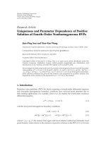
Figure 4: Theoretical and simulation results of the one-stage A PIC
receiver, N
= 32, SNR = 20 dB.
5. NUMERICAL RESULTS AND DISCUSSIONS
In this section, the performance of the APIC receiver for the
MC-DS-CDMA system is studied through numerical results.
The channel is frequency-selective with L

= 3. The number
of identical-bit streams M and parallel-bit branches P should
be chosen to satisfy (3) in order to guarantee flat fading on

each subcarrier. M is referred to as the repetition depth in
[2] which bears the tradeoff between the maximum number
of users supportable and the achievable frequency diversity,
given a fixed number of subcarriers. In the simulations we set
M
= 2 to reflect a certain level of diversity gain. The selection
of P,aslongasitsatisfies(3), does not affect the performance
much although it is constr ained by the total available band-
width as well as the system complexity. Considering that the
practical cell specific scrambling codes could destroy the or-
thogonality between users’ spreading codes, we utilize ran-
dom codes as the spreading codes in the simulations.
In Figure 4, the analytical and simulation results of the
APIC receiver are presented. The dashed curve is numeri-
cally calculated using (26), (27), (28), and (43), wh ere the
MSE of the MAI estimation is obtained from the approxi-
mation of (44). The step-size and the initial weight for the
APIC receiver are μ
= 0.1andw = 1, respectively. There is
a small discrepancy between the theoretical and the simula-
tion results, due to the approximation of the MSE. However,
it can be seen that if the MSE is obtained from the simula-
tions, the resultant BER calculated from the equations is very
close to the statistic BER obtained from the Monte Carlo sim-
ulations. Under the same settings, Figure 5 illustrates the an-
alytical and simulation results of both the APIC and CPIC re-
ceivers in terms of BER versus SNR. The derivations of both
0 5 10 15 20 25 30
SNR (dB)
10

−3
10
−2
10
−1
10
0
BER
CPIC-analytic
CPIC-simulation
APIC-analytic
APIC-simulation
Figure 5: Analytical and simulation results of the one-stage CPIC
and APIC receivers, N
= 32, K = 30. APIC-analytic uses the simu-
lated MSE.
receivers are justified through the agreement of the analytical
and simulation results.
For the adaptive receiver, the step-size μ plays an impor-
tant role in system performance. In the sequel, simulations
are conducted to investigate the effects of the step-size and
the initial weights on the performance of the APIC receiver.
It is shown in Figure 6 that the lowest BER is achieved when
the initial weight is w
0
= 1atμ = 0.3. Note that when the
initial weight is w
0
= 1 and the step-size is μ = 0, the APIC
reduces to the CPIC. The horizontal line in the figure repre-

sents the perfor mance of the CPIC receiver, and we can see
that the APIC outperforms the CPIC for μ
∈ (0, 0.5).
Under the same simulation settings, the BER perfor-
mances of the one- and two-stage APIC receiver versus the
step-size μ are presented in Figure 7. The initial weight has
been fixed at 1. It is shown that the one-stage APIC receiver
achieves its best performance at μ
= 0.3. However, for the
two-stage APIC receiver (with the step-size of the first stage
being μ
1
= 0.3), the best performance is at the point where
μ
2
= 0. Hence the APIC reduces to the CPIC at the sec-
ond stage (horizontal line). The underlying reason lies in the
fact that, for both the APIC and the CPIC, the MAI estima-
tion has been reliable enough after the first stage processing.
Hence the APIC does not have superiority over the CPIC at
the second stage. However, when the SNR is low or the sys-
tem load is heavy such that the first stage cannot perfectly
handle the MAI estimation errors, a small nonzero step-size
for the second stage guarantees advantage of the APIC over
the CPIC. This is verified in Figure 8, where for the APIC, the
first stage adopts a step-size of μ
1
= 0.3andμ
2
= 0.05 for the

second stage.
Furthermore, the influence of the choice of the initial
weight w
0
is shown in Figure 9, where the MSE performances
8 EURASIP Journal on Wireless Communications and Networking
00.511.5
Step-size μ
10
−3
10
−2
10
−1
BER
APIC, w = 0
APIC, w
= 1.5
APIC, w
= 0.5
APIC, w
= 1
Performance of CPIC
Figure 6: BER performance of one stage APIC receiver with differ-
ent initial weights as a function of the step-size, N
= 32, SNR =
20 dB, K = 30.
00.511.5
Step-size μ
10

−4
10
−3
10
−2
10
−1
BER
APIC, first stage with initial w eight w
0
= 1
APIC, second stage with initial w eight w
0
= 1andμ
1
= 0.3
Performance of CPIC, first stage
Performance of CPIC, second stage
Figure 7: BER performance of the first and second stage of the
APIC as a function of the step-size.
with different initial weights are presented. It is shown
that when the initial weight is randomly chosen, it takes a
while for the algorithm to converge. Consequently, when the
processing gain of the system is small, the algorithm con-
verges across multiple symbols. A ver y natural choice of the
initial weight for the proposed scheme, however, is w
0
= 1.
The idea comes with the obvious fact that by choosing w
0

=
1, the algorithm starts from the CPIC, which constitutes a
stationary starting point.
20 30 40 50 60 70 80
Number of users (K)
10
−5
10
−4
10
−3
10
−2
10
−1
BER
1stage-CPIC
1stage-APIC
2stage-CPIC
2stage-APIC
Figure 8: BER performances of the CPIC versus the APIC. N = 32,
SNR
= 20 dB. For the APIC, μ
1
= 0.3, μ
2
= 0.05.
0 50 100 150 200 250 300
Iterations (n)
0

0.01
0.02
0.03
0.04
0.05
0.06
0.07
MSE
w
0
= 0
w
0
= 0.5
w
0
= 1
Figure 9: Convergence comparison for different initial weights.
N
= 32, K = 30, SNR = 20 dB, μ = 0.3.
6. CONCLUSIONS
In this paper, we designed an adaptive receiver for the multi-
carrier DS-CDMA system over Rayleigh fading channels and
evaluated the performance of the system. A closed form ex-
pression of the BER is originally derived for the APIC re-
ceiver, and it was shown that the derivation of the BER for
the CPIC receiver can be unified under the same frame-
work. Simulation results are provided to verify the theoretical
Huahui Wang et al. 9
derivations. The effect of the design parameters of the APIC

receiver, such as the adaptive step-size and the initial weights,
are investigated. It is shown that with the appropriate selec-
tion of these parameters, the APIC outperforms the CPIC.
APPENDIX
At the MAI estimation stage, the regenerated signal of the nth
chip corresponding to the qth carrier given in (12)isrewrit-
ten here for convenience of reference:
s
(k)
q
(n) =

P
k
2M

d
(k)
p
c
(k)
(n)ζ
(k)
q
,1≤ m ≤ M. (A.1)
Stack K users’ signals in one vector as
s(n)
=

s

(1)
q
(n), s
(2)
q
(n), , s
(K)
q
(n)

T
,(A.2)
such that the K
× K autocorrelation matrix is defined as
R
= E

s(n) s
T
(n)

. (A.3)
Under ideal power control, the channel is statistically
identical for all users. The average power received at the base
station for users can be assumed to be equal. By normalizing
E[P
k
|ζ
(k)
q

|
2
] = 1, for all k = 1, 2, , K, and incorporating
the i.i.d s ource data assumption made in Section 4, we then
have the following result:
R
=
⎡
⎢
⎢
⎢
⎢
⎢
⎢
⎢
⎢
⎢
⎣
1
2MN
0
··· 0
0
1
2MN
··· 0
.
.
.
···

.
.
.
.
.
.
00
···
1
2MN
⎤
⎥
⎥
⎥
⎥
⎥
⎥
⎥
⎥
⎥
⎦
=
1
2MN
I
K
,(A.4)
where I
K
is the K × K unit matrix. The inverse of the matrix

R is given by
R
−1
= 2MNI
K
. (A.5)
As in (7), the reference signal is given by
r
q
(n) =
K

k=1
v
(k)
q
(n)+η
t
(n), 0 ≤ n ≤ N − 1, (A.6)
thus we can define the K
× 1 cross-correlation vector
p
= E

s(n)r
∗
q
(n)

. (A.7)

It is then easy to obtain the minimum mean-square error
(MMSE) of the MAI estimation as [29]
ε
min
= E



r
q
(n)


2

−
p
H
R
−1
p. (A.8)
The equal power and the i.i.d source data assumptions
further lead to the following result:
E



r
q
(n)



2

=
E






K

k=1
v
(k)
q
(n)+η
t
(n)





2

=
K


k=1
E







P
k
2M
d
(k)
p
c
(k)
(n)ζ
(k)
q





2

+ σ
2

η
=
K
2MN
+ σ
2
η
,
(A.9)
where σ
2
η
= N
0
/2.
From (A.1), (A.6) and the expression of v
(k)
q
(n)in(8), we
can easily calculate the kth component of p as
E

s
(k)
q
(n)r
∗
q
(n)


=
1
2MN
E


d
(k)
p
d
(k)
p

=
1 − 2P
ini
[e]
2MN
.
(A.10)
Hence, the cross-correlation vector p is given by
p
=
1 − 2P
ini
[e]
2MN

11··· 1



 
K
T
. (A.11)
The MMSE in (A.8) can then be written as
ε
min
=
K

1 −

1 − 2P
ini
[e]

2

2MN
+ σ
2
η
. (A.12)
When the LMS algorithm [29] is utilized for adaptive signal
processing, the mean-square error (MSE) of the estimation
can be separated into two terms as
MSE
= ε
min

+ ε
excess
, (A.13)
where ε
excess
is the excess MSE which is proportional to ε
min
,
that is,
ε
excess
= λ · ε
min
. (A.14)
Assuming that the step-size μ is properly selected such that
the misadjustment of the LMS algorithm is less than 10%,
that is, λ
≤ 0.1, we have
λ
=
μ · tr[R]
1 − μ · tr[R]
≈ μ · tr[R] =
μK
2MN
. (A.15)
Finally, the expression of the MSE is given by
MSE
= (1 + λ) · ε
min

=

1+
μK
2MN

K

1 −

1 − 2P
ini
[e]

2

2MN
+ σ
2
η

.
(A.16)
10 EURASIP Journal on Wireless Communications and Networking
ACKNOWLEDGMENT
The authors would like to thank the anonymous reviewers
for their valuable comments.
REFERENCES
[1] L. Hanzo, L L. Yang, E L. Kuan, and K. Yen, Single- and
Multi-Carrier DS-CDMA: Multi-User Detection, Space-Time

Spreading, Synchronisation, Standards and Networking,John
Wiley & Sons, New York, NY, USA, 2003.
[2] L L. Yang and L. Hanzo, “Multicarrier DS-CDMA: a multiple
access scheme for ubiquitous broadband wireless communi-
cations,” IEEE Communications Magazine, vol. 41, no. 10, pp.
116–124, 2003.
[3] J. A. C. Bingham, “Multicarrier modulation for data transmis-
sion: an idea whose time has come,” IEEE Communications
Magazine, vol. 28, no. 5, pp. 5–14, 1990.
[4] E. A. Sourour and M. Nakagawa, “Performance of orthogo-
nal multicar rier CDMA in a multipath fading channel,” IEEE
Transactions on Communications, vol. 44, no. 3, pp. 356–367,
1996.
[5] S. Hara and R. Prasad, “Overview of multicarrier CDMA,”
IEEE Communications Magazine, vol. 35, no. 12, pp. 126–133,
1997.
[6] N. Yee, J P. Linnartz, and G. Fettweis, “Multi-carrier CDMA
for indoor wireless radio networks,” in Proceedings of the IEEE
International Symposium on Personal, Indoor and Mobile Ra-
dio Communications (PIMRC ’93), pp. 109–113, Yokohama,
Japan, September 1993.
[7] V. DaSilve and E. S. Sousa, “Performance of orthogonal
CDMA codes for quasi-synchronous communication sys-
tems,” in Proceedings of the 2nd International Conference on
Universal Personal Communications (ICUPC ’93), vol. 2, pp.
995–999, Ottawa, Canada, October 1993.
[8] L. Vandendorpe, “Multitone direct sequence CDMA system
in an indoor wireless environment,” in Proceedings of the 1st
IEEE Symposium on Communications and Vehicular Technol-
og y (SCVT ’93), pp. 4.1-1–4.1-8, Delft, The Netherlands, Oc-

tober 1993.
[9] K. Fazel, S. Kaiser, and M. Schnell, “A flexible and high perfor-
mance cellular mobile communications system based on or-
thogonal multi-carrier SSMA,” Wireless Personal Communica-
tions, vol. 2, no. 1-2, pp. 121–144, 1995.
[10] T. M
¨
uller, H. Rohling, and R. Gr
¨
unheid, “Comparison of dif-
ferent detection algorithms for OFDM-CDMA in broadband
Rayleigh fading,” in Proceedings of the 45th IEEE Vehicular
Technology Conference (VTC ’95), vol. 2, pp. 835–838, Chicago,
Ill, USA, July 1995.
[11] S. Kaiser, “OFDM-CDMA versus DS-CDMA: performance
evaluation for fading channels,” in Proceedings of IEEE Inter-
national Conference on Communications (ICC ’95), vol. 3, pp.
1722–1726, Seattle, Wash, USA, June 1995.
[12] S. Kaiser, “On the performance of different detection tech-
niques for OFDM-CDMA in fading channels,” in Proceed-
ings of IEEE Global Telecommunications Conference (GLOBE-
COM ’95), vol. 3, pp. 2059–2063, Singapore, November 1995.
[13] S. Hara and R. Prasad, “DS-CDMA, MC-CDMA and MT-
CDMA for mobile multi-media communications,” in Proceed-
ings of the 46th IEEE Vehicular Technology Conference (VTC
’96), vol. 2, pp. 1106–1110, Atlanta, Ga, USA, April-May 1996.
[14] S. Kondo and B. Milstein, “Performance of multicarrier
DS CDMA systems,” IEEE Transactions on Communications,
vol. 44, no. 2, pp. 238–246, 1996.
[15] W. Xu and L. B. Milstein, “On the performance of multicar-

rier RAKE systems,” IEEE Transactions on Communications,
vol. 49, no. 10, pp. 1812–1823, 2001.
[16] S. Moshavi, “Multi-user detection for DS-CDMA communi-
cations,” IEEE Communications Magazine, vol. 34, no. 10, pp.
124–136, 1996.
[17] S. Verd
´
u, Multiuser Detection, Cambridge University Press,
New York, NY, USA, 1998.
[18] S. Verd
´
u, “Adaptive multiuser detection,” in Proceedings of the
3rd IEEE International Symposium on Spread Spectrum Tech-
niques & Applications, vol. 1, pp. 43–50, Oulu, Finland, July
1994.
[19] M. L. Honig and H. V. Poor, “Adaptive interference suppres-
sion,” in Wireless Communications: Signal Processing Perspec-
tives, pp. 64–128, Prentice-Hall, Upper Saddle River, NJ, USA,
1998.
[20] S. J. Chern, C. Y. Chang, and T. Y. Liao, “Adaptive multiuser
interference cancellation with robust constrained IQRD-RLS
algorithm for MC-CDMA system,” in Proceedings of IEEE
International Symposium on Intelligent Signal Processing and
Communication Systems, pp. 242–246, Nashville, Tenn, USA,
November 2001.
[21] L. Fang and L. B. Milstein, “Successive interference cancella-
tion in multicarrier DS/CDMA,” IEEE Transactions on Com-
munications, vol. 48, no. 9, pp. 1530–1540, 2000.
[22] J. G. Andrews and T. H. Y. Meng, “Performance of multicar-
rier CDMA with successive interference cancellation in a mul-

tipath fading channel,” IEEE Transactions on Communications,
vol. 52, no. 5, pp. 811–822, 2004.
[23] M. K. Varanasi and B. Aazhang, “Near-optimum detection
in synchronous code-division multiple-access systems,” IEEE
Transactions on Communications, vol. 39, no. 5, pp. 725–736,
1991.
[24] D. Divsalar, M. K. Simon, and D. Raphaeli, “Improved paral-
lel interference cancellation for CDMA,” IEEE Transactions on
Communications, vol. 46, no. 2, pp. 258–268, 1998.
[25] G. Xue, J. Weng, T. Le-Ngoc, and S. Tahar, “Adaptive multi-
stage parallel interference cancellation for CDMA,” IEEE Jour-
nal on Selected Areas in Communications, vol. 17, no. 10, pp.
1815–1827, 1999.
[26] W. Xu and L. B. Milstein, “Performance of multicarrier DS
CDMA systems in the presence of correlated fading,” in Pro-
ceedings of the 47th IEEE Vehicular Technology Conference
(VTC ’97), vol. 3, pp. 2050–2054, Phoenix, Ariz, USA, May
1997.
[27] A. Kajiwara and M. Nakagawa, “Microcellular CDMA system
with a linear multiuser interference canceler,” IEEE Journal on
Selected Areas in Communications, vol. 12, no. 4, pp. 605–611,
1994.
[28] P. S. Kumar and J. Holtzman, “Power control for a spread spec-
trum system with multiuser receivers,” in Proceedings of the
6th IEEE International Symposium on Personal, Indoor and Mo-
bile Radio Communications (PIMRC ’95), vol. 3, pp. 955–959,
Toronto, Canada, September 1995.
[29] S. Haykin, Adaptive Filter Theory, Prentice-Hall, Upper Saddle
River, NJ, USA, 3rd edition, 1996.
[30] J. Proakis, Digital Communications, McGraw-Hill, New York,

NY, USA, 4th edition, 2001.
[31] Y. C. Yoon, R. Kohno, and H. Imai, “A spread-spectrum mul-
tiaccess system with cochannel interference cancellation for
multipath fading channels,” IEEE Journal on Selected Areas in
Communications, vol. 11, no. 7, pp. 1067–1075, 1993.