Báo cáo hóa học: " Research Article Performance Analysis of Space-Time Block Codes in Flat Fading MIMO Channels with Offsets" potx

Hindawi Publishing Corporation
EURASIP Journal on Wireless Communications and Networking
Volume 2007, Article ID 30548, 7 pages
doi:10.1155/2007/30548
Research Article
Performance Analysis of Space-Time Block Codes in Flat
Fading MIMO Channels with Offsets
Manav R. Bhatnagar,
1
R. Vishwanath,
2
and Vaibhav Bhatnagar
3
1
Depar tment of Informatics, UniK-University Graduate Center, University of Oslo, 2027 Kjeller, Norway
2
Department of Electrical and Computer Engineering, University of California, Davis, CA 95616, USA
3
Department of Electrical Engineering, University of Bridgeport, Bridgeport, CT 06604, USA
Received 19 June 2006; Revised 14 October 2006; Accepted 11 February 2007
Recommended by Yonghui Li
We consider the effect of imperfect carrier offset compensation on the performance of space-time block codes. The symbol error
rate (SER) for orthogonal space-time block code (OSTBC) is derived here by taking into account the carrier offset and the resulting
imperfect channel state information (CSI) in Rayleigh flat fading MIMO wireless channels with offsets.
Copyright © 2007 Manav R. Bhatnagar et al. This is an open access article distributed under the Creative Commons Attribution
License, which permits unrestricted use, distribution, and reproduction in any medium, provided the original work is properly
cited.
1. INTRODUCTION
Use of space-time codes with multiple transmit antennas has
generated a lot of interest for increasing spectral efficiency as
well as improved performance in wireless communications.

Although, the literature on space-time coding is quite rich
now, the orthogonal designs of Alamouti [1], Tarokh et al.
[2, 3], Naguib and Sesh
´
adri [4] remain popular. The strength
of orthogonal designs is that these lead to simple, optimal re-
ceiver structure due to the possibility of decoupled detection
along orthogonal dimensions of space and time.
Presence of a frequency offset between the t ransmitter
and receiver, which could arrive due to oscillator instabilities,
or relative motion between the two, however, has the poten-
tial to destroy this orthogonality and hence the optimality of
the corresponding receiver. Several authors have, therefore,
proposed methods based on pilot symbol transmission [5]or
even blind methods [6] to estimate and compensate for the
frequency offset under different channel conditions. Never-
theless, some residual offset remains, which adversely affects
the code orthogonality and leads to increased symbol error
rate (SER).
The purpose of this paper is to analyze the effect of such a
residual frequency offset on performance of MIMO system.
More specifically, we obtain a general result for calculating
the SER in the presence of imperfect carrier offset knowl-
edge (COK) and compensation, and the resulting imperfect
CSI (due to imperfect COK and noise). The results of [7–12]
which deal with the cases of performance analysis of OSTBC
systems in the presence of imperfect CSI (due to noise alone)
follow as special cases of the analysis presented here.
The outline of the paper is as follows. Formulation of
the problem is accomplished in Section 2.Meansquareer-

ror (MSE) in the channel estimates due to the residual offset
error (ROE) is obtained in Section 3.InSection 4, we dis-
cuss the decoding of OSTBC data. In Section 5, the prob-
ability of error analysis in the presence of imperfect offset
compensation is presented and we discuss the analytical and
simulation results in Section 6. Section 7, contains some con-
clusions and in the appendix we derive the total interference
power in the estimation of OSTBC data.
NOTATIONS
Throughout the paper we have used the following notations:
B is used for matrix, b is used for vector, b
∈ b or B, B and
b are used for variables, [
·]
H
is used for hermitian of matrix
or vector, [
·]
T
is used for transpose of matrix or vector,[I]is
used for identity matrix, and [
·]
∗
is used for conjugate ma-
trix or vector.
2. PROBLEM FORMULATION
2.1. System modeling
Here for simplicity of analysis we restrict our attention to the
simpler case of a MISO system (i.e., one with m transmit and
2 EURASIP Journal on Wireless Communications and Networking

1
m
.
.
.
Tx
h
1
ω
0
.
.
.
h
m
ω
0
Rx
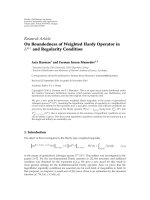
Figure 1: MISO system considered in the problem.
single receive antennas) shown in Figure 1, in which the fre-
quency offset between each of the transmitters and the re-
ceiver is the same, as will happen when the source of fre-
quency offset is primarily due to oscillator drift or platform
motion.
Here h
k
are channel gains between kth transmit antenna
and receive antenna and ω
0
is the frequency offset. The re-

ceived data vector corresponding to one frame of transmitted
data in the presence of carrier offset is given by
y
= Ω

ω
0

Fh + e,(1)
where y
= [y
1
y
2
···y
N
t
+N
]
T
; N
t
and N being the num-
ber of time intervals over which, respectively, pilot sym-
bols and unknown symbols are transmitted, F consists of
data formatting matrix [S
t
S] corresponding to one frame;
S
t

and S being the pilot symbol matrix and space-time ma-
trix, respectively, h
= [
h
1
h
2
··· h
m
]
T
denotes the chan-
nel gain vector w ith statistically independent complex cir-
cular Gaussian components of variance σ
2
, and station-
ary over a frame duration, e is the AWGN noise vector
[e
1
e
2
···e
N
t
+N
]
T
with a power density of N
0
/2 per dimen-

sion, and Ω(ω
0
) = diag{exp(jω
0
), exp( j2ω
0
), ,exp(j(N
t
+
N)ω
0
)} denotes the carrier offset matrix.
2.2. Estimation of carrier offset and imperfect
compensation of the received data
Maximum likelihood (ML) estimation of transmitted data
requires the perfect knowledge of the carrier offset and the
channel. The offset can be estimated through the use of pilot
symbols [5], or using blind method [6]. However, a few pi-
lot symbols are almost always necessary, for estimation of the
channel gains. Considering all this, therefore, we use in our
analysis a generalized frame consisting of an orthogonal pilot
symbol matrix (typically proportional to the identity matrix)
and the STBC data matrix. In any case, the estimation of the
offset cannot be perfect due to the limitations over the data
rate, and delay and processing complexity. There could also
be additional constraint in the form of time varying nature
of the unknown channel. Thus, a residual offset error will al-
ways remain in the received data even after its compensation
based on its estimated value. This can be explained as follows:
if

ω
0
denotes the estimated value of the offset ω
0
,wehave
ω
0
= ω
0
− Δω,(2)
where Δω is a residual offset error (ROE) the amount of
which depends upon the efficiency of the estimator. The
compensatedreceiveddatavectorwillbe
y
c
= Ω

− 
ω
0

y = Ω(Δω)Fh + Ω

− 
ω
0

e. (3)
It is reasonable to consider ROE to be normally dis-
tributed with zero mean and variance σ

2
ω
.Wehavealsoas-
sumed that carrier offset and hence ROE remains constant
over a data frame. The problem of interest here is to analyt-
ically find the performance of the receiver in the presence of
ROE.
3. MEAN SQUARE ERROR IN THE ESTIMATION OF
CHANNEL GAINS IN THE PRESENCE OF RESIDUAL
OFFSET ERROR
Although it is possible to continue with the general case of m
transmit antennas, the treatment and solution becomes cum-
bersome, especially since the details will also depend on the
specific OSTBC used. On the other hand, the principle be-
hind the analysis can be easily illustrated by considering the
special case of two transmit antennas, employing the famous
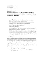
Alamouti code [1]. Suppose we transmit K orthogonal pilot
symbol blocks of 2
× 2 size and L Alamouti code blocks over
a frame. One such frame is depicted in Figure 2,wherex is a
pilot symbol of unit power and s
r
(k) represents the rth sym-
bol transmitted by the kth antenna and x, s
r
(k) ∈ M-QAM.
The compensated received vector corresponding to K
training data blocks (denoted here by matrix P)canbeex-
pressed as


y
c
=

y
1
c
y
2
c
···y
2K
c

T
= Ω(Δω)
2K×2K
Ph + Ω

− ω
0

2K×2K
e
2K×1
,
(4)
where Ω(Δω)
2K×2K
is the ROE matrix and Ω(−ω

0
)
2K×2K
is
compensating matrix, respectively, corresponding to K pilot
blocks, and e
2K×1
is the noise in pilot data. It may be noted
that the last term in (4) can still be modeled as complex,
circular Gaussian and contains independent components. As
the receiver already has the information about P,wecanfind
the ML estimate of the channel gains as follows [2, 4]:

h =
1
K|x|
2
P
H

y
c
. (5)
Substituting the value of

y
c
from (4) into (5), we get

h =

1
K|x|
2
P
H
Ω(Δω)
2K×2K
Ph
+
1
K|x|
2
P
H
Ω

− 
ω
0

2K×2K
e
2K×1
.
(6)
In the low mobility scenario where the carrier offset is
mainly because of the oscillator instabilities, its value is very
small and if sufficient training data is transmitted or an effi-
cient blind estimator is used, the variance σ
2

ω
of ROE is gen-
erally very small (σ
2
ω
 1), thus we can comfortably use a
Manav R. Bhatnagar et al. 3
⎡
⎣
x 0 ··· x 0
0 x
··· 0 x
⎤
⎦

 
Training data (K blocks)
⎡
⎣
s
1
(1) s
2
(1) s
3
(1) s
4
(1) ···s
2L−1
(1) s

2L
(1)
−s
∗
2
(2) s
∗
1
(2) −s
∗
4
(2) s
∗
3
(2) ···−s
∗
2L
(2) s
∗
2L−1
(2)
⎤
⎦

 
STBC data (L blocks)
Figure 2: Complete frame for two transmit antennas and single receive antenna case.
first order Taylor series approximation for exponential terms
in Ω(Δω)
2K×2K

as
exp( jNΔω)
= 1+ jNΔω. (7)
After a simple manipulation, we can find the estimates of
channel gains as

h =

h
1
h
2

+

jKΔωh
1
j(1 + K)Δωh
2


 
error due to residual offset
+
1
K|x|
2
P
H
Ω


− 
ω
0

2K×2K
e
2K×1
  
error due to noise
= h + Δh,
(8)
where Δh
= [
jKΔωh
1
j(1+K)Δωh
2
]+(1/K|x|
2
)P
H
Ω(−ω
0
)
2K×2K
e
2K
is
the total error in estimates. It is easy to see that there are

two distinct interfering terms in (8)duetoROEandAWGN
noise. In the previous work [7–12], the interference only due
to the AWGN noise is considered. However, here in (8)we
are also taking into account the effect of the interference due
to ROE. The mean square error (MSE) of channel estimate
in (8) can be found as follows:
MSE
=
1
2
Tr

E
h,Δω,e

ΔhΔh
H

=
1
2
Tr

E
h,Δω,e

jKΔωh
1
j(1 + K)Δωh
2


+
1
K|x|
2
P
H
Ω

− 
ω
0

2K×2K
e
2K×1

·

jKΔωh
1
j(1 + K)Δωh
2

+
1
K|x|
2
P
H

Ω

− 
ω
0

2K×2K
e
2K×1

H

.
(9)
Assuming, elements of h, Δω and elements of e are statis-
tically independent of each other, the expectation of cross
terms will be zero and the MSE would be simplified as
follows:
MSE
=
1
2
Tr

E
h,Δω

jKΔωh
1
j(1 + K)Δωh

2

jKΔωh
1
j(1 + K)Δωh
2

H

+ E
e

1
K|x|
2
P
H
Ω

− 
ω
0

2K×2K
e
2K×1

·

1

K|x|
2
P
H
Ω

− ω
0

2K×2K
e
2K×1

H

=


K
2
+(1+K)
2

2

σ
2
ω
σ
2

+

1
K

N
0
|x|
2

.
(10)
This generalizes the results of mean square channel estima-
tion error in AWGN noise only [7, 8] to the case where there
is also a residual offset present in the data being used for
channel estimation. It is clear that the expression reduces to
that in [7, 8], when σ
2
ω
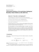
= 0. Figure 3 depicts the results in a
graphical form for two pilot blocks. It is also satisfying to see
that the results match closely (except very large ROEs) those
based on experimental simulations. The effect of σ
2
ω
is seen
to be very prominent as it introduces a floor in MSE value,
independent of SNR.
4. ESTIMATION OF OSTBC DATA
Next, we consider the compensated received data vector cor-

responding to the OSTBC part of the frame. Consider the lth
STBC (Alamouti) block, which can be written as [1]
z
=

y
(2v−1)
c

y
2v
c

∗

T
=

e
j(2v−1)Δω
0
0 e
−j2vΔω

Hs
+

e
j(2v−1) ω
0

0
0 e
−j2v ω
0


e
2v−1
e
∗
2v

T
,
(11)
where v
= K + l, H = [
h
1
h
2
h
∗
2
−h
∗
1
], and s = [
s
2l−1

s
2l
]
T
. If the
channel is known perfectly, then the ML estimation rule for
obtaining estimate of s is given as
s = arg min r − ρs, (12)
4 EURASIP Journal on Wireless Communications and Networking
10
−4
10
−3
10
−2
10
−1
10
0
Mean square error (MSE)
0 5 10 15 20 25 30
SNR
Analysis
Simulation
Figure 3: Analytical and experimental plots of MSE in the chan-
nel estimates for differentvaluesofROE;σ
2
ω
= (2π/30)
2

,(2π/50)
2
,
(2π/100)
2
,(2π/250)
2
,(2π/1000)
2
, 0 from uppermost to downmost,
respectively.
where
ρ
= H
H
H, r = H
H
z. (13)
In the presence of channel estimation errors, as discussed in
Section 3, the vector r will be equal to
r
=

H
H
z = (H + ΔH)
H
z, (14)
where ΔH
= [

Δh
1
Δh
2
Δh
∗
2
−Δh
∗
1
]. Substituting the value of z from
(11) into (14), we get
r
=

H
H

e
j(2v−1)Δω
0
0 e
−j2vΔω


 
I
Hs
+


e
j(2v−1) ω
0
0
0 e
−j2v ω
0


e
(2v−1)
e
∗
2v

T

.
(15)
Applying Taylor series approximation for the exponential
term in the term (I) in (15), we wil l get
r
=

H
H
Hs +

H
H


j(2v − 1)Δω 0
0
−j2vΔω

Hs
+

H
H

e
j(2v−1) ω
0
0
0 e
−j2v ω
0


e
2v−1
e
∗
2v

T
.
(16)
From (14)and(16), r can be expressed as

r
= ρs + ΔH
H
Hs
  
interfering term (1)
+

H
H
H
Ω
s
  
interfering term (2)
+

H
H

e
j(2v−1) ω
0
0
0 e
−j2v ω
0


e

(2v−1)
e
∗
2v

T
  
interfering term (3)
,
(17)
where H
Ω
= [
j(2v−1)Δω 0
0
−j2vΔω
]H. Clearly, estimation of s via
minimization of (12) would be affected by the interfering
terms (1)–(3) shown in (17). In the next section, we carry
out an SER analysis by first obtaining expression for the total
interference power and its subsequent effect on the signal-to-
interference ratio (SIR).
5. ERROR PROBABILITY ANALYSIS
In order to obtain an expression for the SIR, and hence for
the probability of error, we need to find the total interference
power in (17). To simplify the analysis, we restrict ourself to
those cases when ω
0
is typically much smaller than the sym-
bol period and if a sufficiently efficient estimator like [5, 6]is

used for carrier offset estimation, Δω is also very less than the
symbol period. Under this restriction and assuming channel,
noise, training data and S-T data independent of each other
and of zero mean, the correlations between Δh and h, Δh and
Δω,and

H and H
Ω
, which mainly depend upon ω
0
and Δω,
would be so small that these could be neglected. We make
use of this assumption in the following analysis for simplic-
ity, but without any loss of generality. In this case, the total
interference power in (17) is obtained in the appendix and
the average interfering power will be
Power
avg
= 2E
s
σ
2
MSE +2(2v − 1)
2
E
s
σ
2
ω
σ

2

σ
2
+MSE

+2

σ
2
+MSE

N
0
.
(18)
Since the channel is modeled as complex Gaussian random
variable with variance σ
2
,henceE{

m
i
=1
|h
i
|
2
}=mσ
2

and
the average SIR per channel wil l be
γ =
E
s
2Power
avg
σ
2
=
E
s
2

E
s
σ
2
MSE+(2v−1)
2
E
s
σ
2
ω
σ
2

σ
2

+MSE

+

σ
2
+MSE

N
0

σ
2
,
(19)
where E
s
is signal power. If there is no carrier offset present,
that is, σ
2
ω
=0, and channel variance is unity, that is, σ
2
=1, (19)
reduces into the following conventional form [7–12]:
γ =
E
s
2


E
s
MSE +N
0
+ N
0
MSE

. (20)
Hence, (19) is more general form of SIR than (20) and there-
fore, our analysis presents a comprehensive view of the be-
havior of STBC data in the presence of carrier offset. Further,
Manav R. Bhatnagar et al. 5
the expression of exact probability of error for M-QAM data
received over J-independent flat fading Rayleigh channels, in
the terms of SIR, is suggested in [13]as
P
e
= 4

1 −
1
√
M

1 − μ
c
2

J

J
−1

l=0

J −1+l
l


1+μ
c
2

J
− 4

1 −
1
√
M

2
·
⎛
⎝
1
4
−
μ
c

π
⎛
⎝

π
2
− arctan μ
c

J−1

l=0

2l
l

4

1+g
QAM
γ

l
− sin

arctan μ
c

J−1


l=1
l

i=1
T
il

1+g
QAM
γ

l
·

cos

arctan μ
c

2(l−i)+1
⎞
⎠
⎞
⎠
,
(21)
where
μ
c
=


g
QAM
γ
1+g
QAM
γ
, g
QAM
=
3
2(M − 1)
,
T
il
=

2l
l


2(l − i)
(l
− i)

4
i

2(l − i)+1



.
(22)
Probability of error in the frame consisting of L blocks of OS-
TBC data will be
P
e
=
1
L
L

i=1

P
e

i
, (23)
where (P
e
)
i
denote the error probability of ith OSTBC block.
As all the interference terms in (17) consist of Gaussian data
and have zero mean and diagonal covariance matrices (see
the appendix), we may assume without loss of generality that
all the interference terms are Gaussian distributed with zero
mean and certain diagonal covariance matrices.
6. ANALYTICAL AND SIMULATION RESULTS

The analytical and simulation results for a frame consisting
of two pilot blocks and three OSTBC blocks are shown in
Figures 4–6. All the simulations are performed with the 16-
QAM data. The average power transmitted in a time interval
is kept unity. The MISO system of two transmit antennas and
a single receive antenna employs Alamouti code. The chan-
nel gains are assumed circular, complex Gaussian with unit
variance and stationary over one frame duration (flat fad-
ing). The analytical plots of SIR and probability of error are
plotted under the same conditions as those of experiments.
Figure 4 shows the effect of ROE on the average SIR per
channel with
−30 dB MSE, in channel estimates. Here, we
have plotted (19)withdifferent values of ROE. It is easy to
see that there is not much improvement in SIR with the in-
crease in SNR at large values of ROE, which is quite intu-
itive. Hence, our analytical formula of SIR presents a feasible
−5
0
5
10
15
20
25
Average SIR per channel
0 5 10 15 20 25 30
SNR
MSE
=−30 dB
Figure 4: Plot of average SIR per channel versus SNR for MSE =

−
30 dB (graphs are plotted for σ
2
ω
= 0, (2π/1000)
2
,(2π)
2
/10
5
,
(2π/100)
2
from uppermost to downmost, resp.).
10
−4
10
−3
10
−2
10
−1
10
0
SER
0 5 10 15 20 25 30
SNR
Analysis
Simulation
Figure 5: SER versus SNR plots for 16 QAM, with no MSE

(graphs are plotted for σ
2
ω
= (2π)
2
/10000, (2π)
2
/20000, (2π/200)
2
,
(2π/300)
2
,(2π/500)
2
,(2π/1000)
2
, 0 from uppermost to downmost,
resp.).
view of the behavior of OSTBC imperfect knowledge of car-
rier offset in MIMO channels.
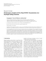
Figures 5 and 6 show the analytical and experimental,
probability of error plots with different values of MSE in
channel estimates and with different values of ROE. It is very
much satisfying to see that the analytical results match closely
those based on experimental simulations for small value of
residual carrier offsets. However, for the large values of off-
set error, the analytical results do not follow the simulation
results very tightly because our assumption of uncorrelated-
ness between different quantities (Section 5) gets violated in
6 EURASIP Journal on Wireless Communications and Networking

10
−4
10
−3
10
−2
10
−1
10
0
SER
0 5 10 15 20 25 30
SNR
Analysis
Simulation
Figure 6: SER versus SNR plots for 16 QAM, with MSE =−40 dB
(graphs are plotted for σ
2
ω
= (2π)
2
/20000, (2π)
2
/80000, (2π/500)
2
,
(2π/1000)
2
from uppermost to down most, resp.).
such cases. Nevertheless, our analysis is still able to provide

an approximate picture of the behavior of the S-T data with
largeresidualoffset errors.
7. CONCLUSIONS
We have performed a mathematical analysis of the behavior
of orthogonal space-time codes with imperfect carrier off-
set compensation in MIMO channels. We have considered
the effect of imperfect carrier offset knowledge over the esti-
mates of the channel gains and resulting probability of error
in the final decoding of OSTBC data. Our analysis also in-
cludes the effect of imperfect channel state information due
to AWGN noise, over the decoding of OSTBC data. Hence, it
presents a comprehensive view of the performance of OSTBC
with imperfect knowledge of small carrier offsets (in case of
small oscillator drifts or low mobility and an efficient offset
estimator) in flat fading MIMO channels with offsets. The
proposed analysis can also predict the approximate behavior
of S-T data with large carrier offsets (in case of high mobility
or highly unstable oscillators and an inefficient offset estima-
tor).
APPENDIX
A. DERIVATION OF TOTAL INTERFERENCE POWER IN
THE ESTIMATION OF OSTBC DATA
We will find the expression of the total interference power in
(17) here. There are three interfering terms in (17). Initially,
we will calculate power of each term separately and finally we
will sum the power of all terms to find the total interference
power. Before proceeding to the power calculation, we can
also assume s being a vector of statistically independent sym-
bols, which are also independent of channel, car rier offset,
channel estimation error, and ROE.

A.1. Power of first interfering term
In view of the discussion of Section 5,wecanwrite
E

ΔH
H
Hs

=
E

ΔH
H

E{H}E{s}=0, (A.1)
implying that the first term has zero mean. Further, it can
be shown that E
{ss
H
}=(E
s
/2)[I], E{HH
H
}=2σ
2
[I]and
E
{ΔH
H
ΔH}=2(MSE)[I], where [I] is identity matrix of

2
× 2. In view of the uncorrelatedness assumption of ΔH,
H and s, and using the results of [14], the covariance matrix
associated with this term can be found as follows:
E

ΔH
H
Hs

ΔH
H
Hs

H

=
E

ΔH
H

E

H

E

ss
H


H
H

ΔH

=
2E
s
σ
2
(MSE)

10
01

.
(A.2)
A.2. Power of second interfering term
The mean of the second interfering term, as per the discus-
sion of Section 5,willbe
E


H
H
H
Ω
s


=
E


H
H

E

H
Ω

E{s}=0, (A.3)
implying that the second term also has zero mean. Further,
it can be show n that E
{H
Ω
H
H
Ω
}
∼
=
2(2v − 1)
2
σ
2
ω
σ
2

[I]and
E
{

H
H

H}=2(σ
2
+MSE)[I]. In view of the uncorrelatedness
assumption of

H, H
Ω
and s, and using the results of [14], the
covariance matrix associated with this term can be found as
follows:
E


H
H
H
Ω
s


H
H
H

Ω
s

H

=
E


H
H

E

H
Ω

E

ss
H

H
H
Ω


H

=

2(2v − 1)
2
E
s
σ
2
ω
σ
2

σ
2
+MSE


10
01

.
(A.4)
A.3. Power of third interfering term
Assuming e,

H and ω
0
being statistically independent of each
other, the mean of the third interfering term will be
E



H
H

e
j(2v−1) ω
0
0
0 e
−j2v ω
0


e
(2v−1)
e
∗
2v

T

=
E


H
H

E

e

j(2v−1) ω
0
0
0 e
−j2v ω
0

E


e
(2v−1)
e
∗
2v

T

=
0,
(A.5)
implying that the third term also has zero mean. Further, it
can be shown that
E

e
(2v−1)
e
∗
2v



e
∗
(2v−1)
e
2v


=
N
0
[I],
E

e
j(2v−1) ω
0
0
0 e
−j2v ω
0

e
−j(2v−1) ω
0
0
0 e
j2v ω
0


=
[I].
(A.6)
Manav R. Bhatnagar et al. 7
Using the results of [14], the covariance matrix can be found
as follows:
E
⎧
⎨
⎩


H
H

e
j(2v−1) ω
0
0
0 e
−j2v ω
0


e
(2v−1)
e
∗
2v


T

×


H
H

e
j(2v−1) ω
0
0
0 e
−j2v ω
0


e
(2v−1)
e
∗
2v

T

H
⎫
⎬
⎭

=
E


H
H

E

e
j(2v−1) ω
0
0
0 e
−j2v ω
0

×

E

e
(2v−1)
e
∗
2v


e
∗

(2v−1)
e
2v


×

e
−j(2v−1) ω
0
0
0 e
j2v ω
0


H

=
2

σ
2
+MSE

N
0

10
01


.
(A.7)
Apparently, all interfering terms are distributed identi-
cally with zero mean and their covariance matrices are pro-
portional to the identity matrix. Further, we note that the
power in the three terms can be simply added, since, these
can be shown to be mutually uncorrelated. Hence, the total
interfering power will be
Power
tot
= 2E
s
σ
2
MSE

10
01

+2(2v − 1)
2
E
s
σ
2
ω
σ
2


σ
2
+MSE


10
01

+2

σ
2
+MSE

N
0

10
01

.
(A.8)
ACKNOWLEDGMENT
The authors are extremely thankful to Professor Are
Hjørungnes, UniK, University of Oslo, for his help provided
in the derivation of the expectation in the appendix.
REFERENCES
[1] S. M. Alamouti, “A simple transmit diversity technique for
wireless communications,” IEEE Journal on Selected Areas in
Communications, vol. 16, no. 8, pp. 1451–1458, 1998.

[2] V. Tarokh, N. Seshadr i, and A. R. Calderbank, “Space-time
codes for high data rate wireless communication: performance
criterion and code construction,” IEEE Transactions on Infor-
mation Theory, vol. 44, no. 2, pp. 744–765, 1998.
[3] V. Tarokh, H. Jafarkhani, and A. R. Calderbank, “Space-time
block codes from orthogonal designs,” IEEE Transactions on
Information Theory, vol. 45, no. 5, pp. 1456–1467, 1999.
[4] A.F.Naguib,N.Sesh
´
adri, and A. R. Calderbank, “Increasing
data rate over wireless channels,” IEEE Signal Processing Mag-
azine, vol. 17, no. 3, pp. 76–92, 2000.
[5] O. Besson and P. Stoica, “On parameter estimation of MIMO
flat-fading channels with frequency offsets,” IEEE Transactions
on Signal Processing, vol. 51, no. 3, pp. 602–613, 2003.
[6] M. R. Bhatnagar, R. Vishwanath, and M . K. Arti, “On blind
estimation of frequency offsets in time varying MIMO chan-
nels,” in Proceedings of t he 3rd IEEE and IFIP International
Conference on Wireless and Optical Communications Networks
(WOCN ’06), p. 5, Bangalore, India, April 2006.
[7] L. Tao, L. Jianfeng, H. Jianjun, and Y. Guangxin, “Performance
analysis for orthogonal space-time block codes in the absence
of perfect channel state information,” in Proceedings of the 14th
IEEE International Symposium on Personal, Indoor and Mobile
Radio Communications (PIMRC ’03), vol. 2, pp. 1012–1016,
Beijing, China, September 2003.
[8] E. Ko, C. Kang, and D. Hong, “Effect of imperfect channel in-
formation on M-QAM SER performance of orthogonal space-
time block codes,” in Proceedings of the 57th IEEE Semiannual
Vehicular Technology Conference (VTC ’03), vol. 1, pp. 722–

726, Jeju, Korea, April 2003.
[9] E. G. Larsson, P. Stoica, and J. Li, “Orthogonal space-time
block codes: maximum likelihood detection for unknown
channels and unstructured interferences,” IEEE Transactions
on Signal Processing, vol. 51, no. 2, pp. 362–372, 2003.
[10] D. Mavares and R. P. Torres, “Channel estimation error effects
on the performance of STB codes in flat frequency Rayleigh
channels,” in Proceedings of the 58th IEEE Vehicular Technology
Conference (VTC ’03), vol. 1, pp. 647–651, Orlando, Fla, USA,
October 2003.
[11] G. Kang and P. Qiu, “An analytical method of channel es-
timation error for multiple antennas system,” in Proceedings
of IEEE Global Telecommunications Conference ( GLOBECOM
’03), vol. 2, pp. 1114–1118, San Francisco, Calif, USA, Decem-
ber 2003.
[12] H. Cheon and D. Hong, “Performance analysis of space-time
block codes in time-varying Rayleigh fading channels,” in Pro-
ceedings of IEEE International Conference on Acoustics, Speech
and Signal Processing (ICASSP ’02), vol. 3, pp. 2357–2360, Or-
lando, Fla, USA, May 2002.
[13] M S. Alouini and A. J. Goldsmith, “A unified approach for
calculating error rates of linearly modulated signals over gen-
eralized fading channels,” IEEE Transactions on Communica-
tions, vol. 47, no. 9, pp. 1324–1334, 1999.
[14] P. M. H. Janssen and P. Stoica, “On the expectation of the
product of four matrix-valued Gaussian random variables,”
IEEE Transactions on Automatic Control,vol.33,no.9,pp.
867–870, 1988.