Báo cáo hóa học: " Research Article Maximum Likelihood Timing and Carrier Synchronization in Burst-Mode Satellite Transmissions" pot

Hindawi Publishing Corporation
EURASIP Journal on Wireless Communications and Networking
Volume 2007, Article ID 65058, 8 pages
doi:10.1155/2007/65058
Research Article
Maximum Likelihood Timing and Carrier Synchronization in
Burst-Mode Satellite Transmissions
Michele Morelli and Antonio A. D’Amico
Department of Information Engineering, Via Caruso, 56100 Pisa, Italy
Received 4 August 2006; Revised 2 March 2007; Accepted 13 May 2007
Recommended by Alessandro Vanelli-Coralli
This paper investigates the joint maximum likelihood (ML) estimation of the carrier frequency offset, timing error, and carrier
phase in burst-mode satellite transmissions over an AWGN channel. The synchronization process is assisted by a training sequence
appended in front of each burst and composed of alternating binary symbols. The use of this particular pilot pattern results into
an estimation algorithm of affordable complexity that operates in a decoupled fashion. In particular, the frequency offset is mea-
sured first and independently of the other parameters. Timing and phase estimates are subsequently computed through simple
closed-form expressions. The per formance of the proposed scheme is investigated by computer simulation and compared with
Cramer-Rao bounds. It turns out that the estimation accuracy is very close to the theoretical limits up to relatively low signal-to-
noise ratios. This makes the algorithm well suited for turbo-coded transmissions operating near the Shannon limit.
Copyright © 2007 M. Morelli and A. A. D’Amico. This is an open access article distributed under the Creative Commons
Attribution License, which permits unrestricted use, distribution, and reproduction in any medium, provided the original work is
properly cited.
1. INTRODUCTION
Burst transmission of digital data and voice is widely adopted
in satellite time-division multiple-access (TDMA) networks.
In these applications the propagation medium can be reason-
ably modeled as an additive white Gaussian noise (AWGN)
channel and knowledge of carrier frequency, symbol timing,
and carrier phase is necessary for coherent demodulation
of the received waveform. In the presence of nonnegligible
phase noise and/or oscillator instabilities, differential detec-

tion is often employed to overcome the inherent difficulty
posed by the phase estimation process. Even with differen-
tial detection, however, the problem of timing and frequency
offset recovery still remains.
Depending on their topology, synchronization circuits
can be divided into two main categories: feedback and feed-
forward schemes [1, 2]. The former have good tracking ca-
pabilities but exhibit comparatively long acquisitions due to
hang-up phenomena [3–5].Thelatterhaveshorteracqui-
sitions and, accordingly, are better suited for burst-mode
transmissions. In many cases, a preamble of known sym-
bols is appended at the beginning of each burst to assist the
synchronization process. Actually, the use of a preamble al-
lows data-aided (DA) operation and provides better estima-
tion accuracy as compared to a non-data-aided (NDA) ap-
proach. Even so, however, synchronization may prove diffi-
cult, especial ly with turbo-coded modulations operating at
relatively low signal-to-noise ratios (SNRs). Clearly, very ef-
ficient synchronization algorithms are needed in these con-
ditions [6].
The common approach to solve the synchronization
problem in burst-mode transmissions is to estimate the tim-
ing error first, and then use the time-synchronized samples
for frequency and phase recovery. Two prominent feedfor-
ward schemes for NDA timing estimation are investigated
in [7, 8]. In part icular, timing estimates are derived in [7]
by searching for the maximum of an approximate version
of the likelihood function while in [8] the received signal is
sampled at some multiple of the symbol rate and a square-
law nonlinearity (SLN) is employed to wipe the modula-

tion out. As shown in [2], the method in [8]isanefficient
way of maximizing the likelihood function of [7]aslong
as the bandwidth of the complex envelope of the transmit-
ted sig nal does not exceed the signaling rate. Since the use
of a SLN exhibits poor performance in the presence of nar-
rowband signaling, alternative methods employing absolute
value or fourth order-based nonlinearities have been devised
[9]. The main advantage of the timing estimators in [7–9]is
2 EURASIP Journal on Wireless Communications and Networking
that they can operate correctly even in the presence of carrier
frequency offsets (CFOs) as large as 20% of the symbol rate.
Frequency estimation is usually performed by exploiting
the received time-synchronized samples. A large number of
schemes proposed in the past operate in either the frequency
or time domain. The Rife and Boorstyn (R&B) algorithm
[10] belongs to the former class and provides maximum like-
lihood (ML) estimates of frequency and phase errors by look-
ing for the peak of a periodogram. Interpolation techniques
may be employed to find an explicit expression of the peak
location [11]. In the time-domain approach, suitable corre-
lations of the received samples are exploited to compute the
frequency estimates. A representative selection of schemes
derived along this line of reasoning can be found in [12–15].
These methods attain the Cramer-Rao lower bound (CRB) at
intermediate/high SNRs, but exhibit different performance
in terms of estimation range and threshold, that is, the SNR
below which large estimation errors are likely to occur.
A possible drawback of conventional frequency estima-
tion schemes as those discussed in [10, 12–15] is that they all
assume ideal timing synchronization. Their performance is

thus limited by the accuracy of the timing estimator. A DA
algorithm for the joint estimation of the carrier phase, fre-
quency offset, and timing error has been proposed in [16]by
resorting to ML arguments. In order to work properly, how-
ever, the demodulated signal must incur negligible phase ro-
tations during the preamble duration. This poses a stringent
limit to the maximum tolerable CFO, which may prevent the
application of this method to many practical situations.
In the present paper we are concerned with the joint esti-
mation of all synchronization parameters for a burst-mode
satellite system operating over AWGN channels. Since one
distinct feature of packetized transmissions is that synchro-
nization must be achieved as fast as possible, in the follow-
ing we only focus our attention to a feedforward s tructure.
Also, we assume that a preamble of alternating binary sym-
bols is transmitted at the beginning of each burst to facili-
tate the timing estimation task [17]. Our approach is based
on ML methods and leads to a three-step procedure. In
the first step frequency recovery is accomplished through a
mono-dimensional grid search. The estimated CFO is then
exploited in the second step to obtain a closed-form expres-
sion of the timing estimate. The final step is devoted to phase
estimation and can be skipped in case of differential data
detection. Surprisingly, no complicated multidimensional
searches are needed to jointly estimate all the unknown syn-
chronization parameters. Simulations indicate that the pro-
posed estimator is well suited for turbo-coded transmissions
since its accuracy approaches the relevant CRBs even at low
SNR values. However, it should be observed that this advan-
tage is achieved at the price of a higher computational com-

plexity as compared to other existing alternatives.
The paper is organized as follows. In Section 2 we in-
troduce the signal model and formulate the synchronization
problem. Section 3 illustrates the joint ML estimation of the
unknown parameters and discusses in some detail the prac-
tical implementation of the frequency estimator. In Section 4
we derive CRBs to characterize the ultimate accuracy of fre-
quency, timing, and phase estimates. Simulation results are
presented in Section 5 while some conclusions are drawn in
Section 6.
2. SYSTEM MODEL AND PROBLEM FORMULATION
2.1. Statement of the problem
We consider the reverse link of a satellite communication
system and assume a time-division multiple-access (TDMA)
scheme where each earth station transmits bursts of data. The
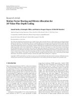
structure of a burst is detailed in Figure 1. Essentially, it con-
sists of two parts: a header section followed by a payload. The
header is further divided in two portions, namely, a synchro-
nization preamble and a unique word (UW). The preamble is
made of a sequence of training sy mbols which are exploited
by the receiver for carrier and symbol timing recovery. The
UW is located just after the preamble and is used for burst
identification as well as to establish the start of the payload.
The first task of the receiver is the start of burst (SoB) de-
tection, that is, the recognition of the time-of-arrival (ToA)
of a generic burst. This is normally performed through a sim-
ple noncoherent energy-detection scheme which provides a
coarse estimate of the position of each burst. Once the SoB
has been identified, the preamble is exploited for carrier and
symbol timing synchronization. This is the second task of the

receiver and represents the focus of our paper. In order to ex-
plain how synchronization can be achieved, we concentrate
on a single burst and assume that the SoB detection algo-
rithm has provided a ToA estimate with an error τ, as shown
in Figure 2. The offset τ can be decomposed as follows:
τ
= ηT − εT,(1)
where T is the symbol period, η is an integer (integer delay),
and ε
∈ [−0.5, 0.5) is a real-valued parameter (fractional de-
lay). Dur ing the preamble we are interested in the estimation
of the fractional delay, because the integer delay is recovered
later by searching for the location of the UW w ithin the burst.
The estimation of the synchronization parameters (fractional
delay, carrier phase, and frequency offsets) is performed by
observing a portion of the preamble of length NT (N is a de-
sign parameter) at the right of the assumed SoB, as shown in
Figure 2. Clearly, the total duration of the preamble has to b e
larger than τ + NT. Since τ is a random variable, this condi-
tion can be practically met by a proper design of the preamble
length. Since we are not concerned with the estimation of the
integer delay, in the fol lowing we set η
= 0.
2.2. Signal model
We consider a linearly modulated digital signal transmitted
over an AWGN channel. The complex envelope of the re-
ceived waveform is modeled as
r(t)
= e
j(2πf

d
t+ϕ)
s(t − εT)+w(t), (2)
where s(t) is the useful signal, ϕ and f
d
are the carrier phase
and frequency offset, respectively, and w(t) is thermal noise
with independent real and imaginary components, each with
M. Morelli and A. A. D’Amico 3
Burst#1 Burst#2 Burst#K
···
Guard
interval
Sync.
preamble
UW
Header Payload
Figure 1: Burst structure.
Sync.
preamble
UW
Payload
τ
NT
Figure 2: Start of burst estimation error.
two-sided power spectral density N
0
. Signal s(t) is expressed
as
s(t)

=

n
a
n
g(t − nT), (3)
where
{a
n
} are modulation symbols taken from a PSK or
QAM constellation and g(t) has a root-raised-cosine Fourier
transform with some roll-off α. To facilitate the timing esti-
mation process, during the preamble we assume a pilot pat-
tern composed by alternating BPSK symbols +1 and
−1[17].
Accordingly, s(t)isgivenby
s(t)
=

2E
s
T
cos

πt
T

(4)
with E
s

denoting the signal energy per symbol interval, and
r(t)mayberewrittenintheform
r(t)
=

2E
s
T
e
j(2πf
d
t+ϕ)
cos

π(t − εT)
T

+ w(t)
for t
∈ [0, NT].
(5)
In order to produce a discrete-time signal, the received
waveform is fed to an anti-aliasing filter (AAF) and sampled
at some rate f
c
. The filter bandwidth B
AAF
and the sampling
rate are chosen such that the signal component is passed
undistorted (even for the maximum frequency offset) and no

aliasing occurs. Assuming that the CFO is less in magnitude
than 0.5/T,from(5) it follows that we can set B
AAF
= 1/T
and f
c
= 2/T. For simplicity, in the ensuing discussion the
AAF is assumed with a brick-wall t ransfer function, even
though the rectangular shape is not strictly necessary and
couldbeeasilymademorerealistic[18].
For normalization purposes, the output of the AAF is
scaled by a factor

T/2E
s
and we call x(k) the correspond-
ing samples taken at t
= kT/2, with 0 ≤ k ≤ 2N − 1. As the
signal is not distorted in passing through the filter, we have
x( k)
=e
j(πkν+ϕ)
cos

k
2
−ε

π


+ n(k)for0≤ k ≤ 2N − 1,
(6)
where ν
= f
d
T is the CFO normalized to the symbol-rate 1/T
and n(k)
= n
R
(k)+jn
I
(k) is the noise contribution. Due to
the previous hypotheses,
{n
R
(k)} and {n
I
(k)} are indepen-
dent and white random sequences with the same variance
σ
2
= (E
s
/N
0
)
−1
. As the signal component in (6) depends on
ν, ε,andϕ, we may estimate all these parameters from the
observation of

{x( k)}. This problem is addressed in the next
section by resor ting to ML methods.
3. MAXIMUM LIKELIHOOD ESTIMATION OF
THE SYNCHRONIZATION PARAMETERS
3.1. Maximization of the likelihood function
Bearing in mind (6), the log-likelihood function for the un-
known parameters is given by
Λ(
ν, ε, ϕ) =−2N ln

2πσ
2

−
1
2σ
2
2N
−1

k=0




x( k) − e
j(πkν+ϕ)
cos

k

2
− ε

π





2
,
(7)
where
ν, ε,andϕ are trial values of ν, ε,andϕ,respec-
tively. The joint ML estimate of (ν, ε, ϕ) is the location wh ere
Λ(
ν, ε, ϕ) achieves its global maximum. Skipping irrelevant
factors and additive terms independent of (
ν, ε, ϕ), it turns
out that Λ(
ν, ε, ϕ) may equivalently be replaced by
Ψ(
ν, ε, ϕ) =e

e
− j ϕ
2N
−1

k=0

x( k)e
− jπkν
cos

k
2
− ε

π


,
(8)
where
e{·} denotes the real part of the enclosed quantity.
Function Ψ(
ν, ε, ϕ) can also be rewritten as
Ψ(
ν, ε, ϕ) =e

e
− j ϕ

Y
e
(ν)cos(πε)+e
− jπν
Y
o
(ν) sin(πε)


(9)
4 EURASIP Journal on Wireless Communications and Networking
with
Y
e
(ν) =
N−1

k=0
(−1)
k
x(2k)e
− j2πkν
,
Y
o
(ν) =
N−1

k=0
(−1)
k
x(2k +1)e
− j2πkν
.
(10)
To ease the search for the maximum of Ψ(
ν, ε, ϕ), we rewrite
(9) in the form

Ψ(
ν, ε, ϕ) =


Z(ν, ε)


cos

ψ(ν, ε) − ϕ

, (11)
where Z(
ν, ε) is a function of ν and ε defined as
Z(
ν, ε) = Y
e
(ν)cos(π ε)+e
− jπν
Y
o
(ν) sin(πε) (12)
while ψ(
ν, ε) = arg{Z(ν, ε)} is the argument of Z(ν, ε).
Clearly, for fixed
ν and ε, the maximum of Ψ(ν, ε, ϕ)is
achieved when the cosine factor in ( 11) is equal to unity,
whichoccursfor
ϕ(ν, ε) = arg


Z(ν, ε)

. (13)
In this case the right-hand side of (11)reducesto
|Z(ν, ε)|
and the ML estimates of ν and ε are found by maximizing the
following function:
Γ(
ν, ε) = 2


Z(ν, ε)


2
(14)
with respect to
ν and ε, where the factor 2 in the right-hand
side of (14) has only been inserted to avoid a factor 1/2 in the
subsequent equations.
To proceed further, we substitute (12) into (14)andob-
tain
Γ(
ν, ε) =


Y
e
(ν)



2
+


Y
o
(ν)


2
+ e

e
− j2πε
A(ν)

, (15)
where A(
ν)isdefinedas
A(
ν) =


Y
e
(ν)


2

−


Y
o
(ν)


2
+2je

e
jπν
Y
e
(ν)Y
∗
o
(ν)

.
(16)
Observing that
|A(ν)|=|Y
2
e
(ν)+e
− j2πν
Y
2

o
(ν)|,wemay
rewrite ( 15) into the equivalent form
Γ(
ν, ε) =


Y
e
(ν)


2
+


Y
o
(ν)


2
+


Y
2
e
(ν)+e
− j2πν

Y
2
o
(ν)


cos

θ(ν) − 2π ε

(17)
with θ(
ν) = arg{A(ν)}.Foragivenν, the maximum of Γ(ν, ε)
is achieved by setting
ε(ν) =
1
2π
arg

A(ν)

. (18)
Substituting this result into the rig ht-hand side of (17) yields
P(
ν) =


Y
e
(ν)



2
+


Y
o
(ν)


2
+


Y
2
e
(ν)+e
− j2πν
Y
2
o
(ν)


(19)
0.50.40.30.20.10−0.1−0.2−0.3−0.4−0.5
ν
0

0.2
0.4
0.6
0.8
1
1.2
P(ν)
E
s
/N
0
= 10 dB
N
= 64
Figure 3: Typical shap e of P(ν).
from which it follows that the ML estimate of the frequency
offset is given by
ν = arg max
ν

P(ν)

(20)
while the timing estimate is obtained from (18) in the form
ε =
1
2π
arg

A(ν)


. (21)
In case of coherent detection, an estimate of the carrier phase
ϕ is also necessary. This is computed as indicated in (13)after
replacing (
ν, ε)by(ν, ε)andreads
ϕ = arg

Y
e
(ν)cos(π ε)+e
− jπν
Y
o
(ν) sin(πε)

. (22)
In the sequel the algorithm based on (20)–(22) is called
the ML estimator (MLE).
3.2. Remarks
(1) Contrarily to what one might fear, the maximization of
the likelihood function Λ(
ν, ε, ϕ) needs not be made on a
three-dimensional domain. Actually, the location (
ν, ε, ϕ)of
the maximum can be found through simple steps, each in-
volving a single synchronization parameter. In particular, the
first step requires maximizing the function P(
ν)definedin
(19) in order to get the CFO estimate

ν. As discussed later,
this can be done through a grid search over the interval where
ν is expected to lie. Once
ν has been obtained, timing and
phase estimates are computed in closed form as indicated
in (21)and(22), respectively. In summary, the difficult and
time-consuming part in the estimation of (ν, ε, ϕ) is the one
that locates the maximum of P(
ν). Once this is done, the
computation of
ε and ϕ becomes a trivial task.
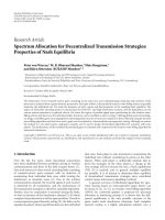
(2) Maximizing function P(
ν) may pose some difficulty
due to the presence of many local maxima. This is clearly ev-
ident from Figure 3, which illustrates a ty pical realization of
M. Morelli and A. A. D’Amico 5
P(ν) as obtained by simulation with N = 64, E
s
/N
0
= 10 dB,
and ν
= 0.1. As discussed in [10], the global maximum can
be sought in two steps. The first one (coarse search) calculates
P(
ν)forasetofν values, say {ν
n
}, covering the uncertainty
range of ν and determines the location
ν

M
of the maximum
over this set. The second step (fine search) makes an inter-
polation between the samples P(
ν
n
) and computes the local
maximum nearest to
ν
M
. It should be noted that the shape
of P(
ν) is occasionally so badly distorted by noise that its
highest peak may be far from the true ν. When this happens,
the MLE makes large errors (outliers) and the system perfor-
mance is highly degraded. The SNR below which the outliers
start to occur is referred to as the threshold of the estimator.
(3) In practice the coarse search can be efficiently per-
formed using fast Fourier transform (FFT) techniques, as it
is now explained. Starting from the observed samples
{x( k)},
we first compute the following zero-padded sequences of
length KN:
y
e
(k) =
⎧
⎨
⎩
(−1)

k
x(2k), 0 ≤ k ≤ N − 1,
0, N
≤ k ≤ NK − 1,
y
o
(k) =
⎧
⎨
⎩
(−1)
k
x(2k +1), 0≤ k ≤ N − 1,
0, N
≤ k ≤ KN − 1,
(23)
where K is a design parameter called pruning factor. Next, the
FFTs of
{y
e
(k)} and {y
o
(k)} are evaluated at the points
ν
n
=
n
KN
,
−

KN
2
≤ n ≤
KN
2
. (24)
This produces the quantities
{Y
e
(ν
n
)} and {Y
o
(ν
n
)},which
are next exploited to get
{P(ν
n
)} as indicated in (19). Finally,
the largest P(
ν
n
) is sought and this provides the coarse fre-
quency estimate.
(4) Collecting (10)and(19), it is seen that P(
ν)isperi-
odic of unit period. This means that MLE gives unambigu-
ousfrequencyestimatesaslongasν is confined within the
interval [

−1/2, 1/2). T his is the frequency estimation range of
MLE.
(5) Compared to the R&B algorithm [10], the MLE is
more complex to implement as it requires the computation
of two FFTs instead of a s ingle FFT. In addition to carrier syn-
chronization, however, the MLE also provides timing recov-
ery. Actually, from (16)and(21) we see that computing the
timing estimate only requires knowledge of Y
e
(ν)andY
o
(ν).
Since these quantities can easily be obtained by
{Y
e
(ν
n
)} and
{Y
o
(ν
n
)} through interpolation, the timing estimation task is
accomplished with a relatively low computational effort once
ν is available. However, it should be observed that the com-
plexity associated to the synchronization process is negligible
compared to that of iterative data decoding [19]. So, the re-
quirement for an additional FFT has only a marginal impact
on the overall receiver complexity.
4. CRB ANALYSIS

By invoking the asymptotic efficiency property of the MLE,
we expect that the accuracy of the estimates (20)–(22)ap-
proaches the corresponding CRBs for relatively large values
of N and E
s
/N
0
. For this reason, it is of interest to derive
the CRB for the joint estimation of the set of parameters
η
= (ν, ε, ϕ) based on the model (6).
We begin by computing the entries of the Fisher infor-
mation matrix F. They are defined as [20]
[F]
i, j
=−E

∂
2
Λ(η)
∂η
i
∂η
j

,1≤ i, j ≤ 3, (25)
where Λ(η) is the log-likelihood function in (7)andη

de-
notes the th entry of η. Substituting (7) into (25), after some

manipulations we obtain
F =
N
6σ
2
⎡
⎢
⎢
⎣
π
2
(2N −1)

4N −1−3cos(2πε)

03π

2N −1−cos(2πε)

06π
2
0
3π

2N −1−cos(2πε)

06
⎤
⎥
⎥

⎦
.
(26)
The CRB for the estimation of η

is given by [F
−1
]
,
. Skip-
ping the details, it is found that
CRB(ν)
=
12

E
s
/N
0

−1
π
2
N

4N
2
− 4+3sin
2
(2πε)


, (27)
CRB(ε)
=

E
s
/N
0

−1
π
2
N
, (28)
CRB(ϕ)
= 2
(2N
− 1)(4N − 1 − 3cosε)

E
s
/N
0

−1
N

4N
2

− 4+3sin
2
(2πε)

. (29)
Interestingly, for large data records we can approximate (27)
as
CRB(ν)
≈
3(E
s
/N
0
)
−1
π
2
N
3
(30)
which represents the CRB for the estimation of the frequency
of a complex sinusoid embedded in AWGN [10].
5. SIMULATION RESULTS
In this section we report on simulation results illustrating the
performance of MLE over an AWGN channel. Unless other-
wise specified, the synchronization parameters vary at each
new simulation run and a re modeled as statistically indepen-
dent random variables with a uniform distribution. In par-
ticular, ν and ε are confined within [
−0.5, 0.5) while ϕ takes

values in the interval [
−π, π). A pruning factor K = 4is
used to compute the quantities
{Y
e
(ν
n
)} and {Y
o
(ν
n
)}. Also,
a parabolic interpolation is chosen in the implementation of
the fine search. This yields a frequency estimate in the form
ν = ν
M
+
δ
ν
2
·
P


ν
M−1

−
P



ν
M+1

P


ν
M−1

−
2P(ν
M
)+P


ν
M+1

, (31)
where δ
ν
= 1/KN is the distance between two adjacent sam-
ples P(
ν
n
) while ν
M
is the output of the coarse search. The
observation length is fixed to either N

= 32 or 64. For
comparison, in the ensuing discussion we also consider a
synchronization scheme in which timing recovery is first ac-
complished by resorting to the Oerder and Meyr (O&M)
6 EURASIP Journal on Wireless Communications and Networking
0.50.40.30.20.10−0.1−0.2−0.3−0.4−0.5
ν
−0.5
−0.4
−0.3
−0.2
−0.1
0
0.1
0.2
0.3
0.4
0.5
E{ν}
E{ν}=ν
E
s
/N
0
= 10 dB
N
= 64
Figure 4: Mean normalized frequency estimates versus ν.
0.50.40.30.20.10−0.1−0.2−0.3−0.4−0.5
ε

−0.5
−0.4
−0.3
−0.2
−0.1
0
0.1
0.2
0.3
0.4
0.5
E{ε}
E{ε}=ε
E
s
/N
0
= 10 dB
N
= 64
Figure 5: Mean timing phase estimates versus ε.
algorithm [8] and carrier synchronization is next achieved
by applying the R&B method [10] to the time-synchronized
samples. The O&M operates with four samples per symbol
period.
Figures 4 and 5 illustrate average frequency and timing
estimates, E
{ν} and E{ε},providedbyMLEasafunctionof
ν and ε, respectively. The observation length is N
= 64 while

the SNR is fixed to E
s
/N
0
= 10 dB. The ideal lines E{ν}=ν
and E
{ε}=ε are indicated as references. These results show
that
ν and ε are unbiased over the full range [−0.5, 0.5).
Figures 6 and 7 compare the mean square error (MSE)
of the timing estimates, E
{(ε − ε)
2
}, as obtained with MLE
and O&M. The observation length is N
= 32 in Figure 6
and N
= 64 in Figure 7. Marks indicate simulation results
while the thin solid lines are drawn to ease the reading of the
graphs. The corresponding CRBs are also shown as bench-
20151050
E
s
/N
0
(dB)
10
−5
10
−4

10
−3
10
−2
10
−1
MSE
ε
O&M
MLE
CRB
N
= 32
Figure 6: MSE performance of MLE and O&M estimator with N =
32.
20151050
E
s
/N
0
(dB)
10
−5
10
−4
10
−3
10
−2
10

−1
MSE
ε
O&M
MLE
CRB
N
= 64
Figure 7: MSE performance of MLE and O&M estimator with N =
64.
marks. We see that MLE has the best accuracy, especially at
low SNRs where a significant gain is observed with respect
to O&M. In particular, for N
= 64 the MLE is close to the
CRB down to E
s
/N
0
values of 0 dB, while O&M approaches
the bound only for E
s
/N
0
> 10 dB. This feature of the MLE
M. Morelli and A. A. D’Amico 7
20151050
E
s
/N
0

(dB)
10
−8
10
−7
10
−6
10
−5
10
−4
10
−3
10
−2
MSE
ν
R&B
MLE
CRB
N
= 64
N
= 32
Figure 8: MSE performance of MLE and R&B estimator with N =
32 and N = 64.
is of great importance as it makes this estimator suitable for
turbo-coded modulations operating at very low SNRs.
Figure 8 illustrates the accuracy of the frequency esti-
mates provided by MLE and R &B with either N

= 32 or
64. Again, the simulation results are compared with the rel-
evant CRBs. We see that the estimation accuracy keeps close
to the CRB down to a certain value of E
s
/N
0
that depends
on the adopted scheme and observation length. If the SNR
is decreased further, a rapid increase in the MSE is observed.
The abscissa at which the slope of the curve starts to change
indicates the estimator threshold and is a manifestation of
the occurrence of outliers. Since large errors have disabling
effects on the system performance, the frequency estimator
must operate above threshold. The results in Figure 8 re-
veal that MLE has a lower threshold than R&B, especially for
N
= 64, which translates into an increased robustness against
outliers. This fact reinforces the idea that for low SNR ap-
plications the MLE is more efficient than other conventional
synchronization schemes. As expected, the threshold is a de-
creasing function of the observation length. Actually, we see
that doubling N results into a threshold decrease of approxi-
mately 3 dB with MLE, while a gain of 2 dB is observed with
R&B.
As mentioned previously, in case of coherent detection
phase recovery is required in addition to frequency and tim-
ing synchronization. The MSE of the phase estimates pro-
videdbyMLEandR&BisillustratedinFigure 9 as a func-
tion of E

s
/N
0
. These results are qualitatively similar to those
in Figure 8. In particular, it turns out that both schemes ap-
proach the CRB at intermediate/high SNR values, but MLE
exhibits a lower threshold than R&B.
20151050
E
s
/N
0
(dB)
10
−3
10
−2
10
−1
10
0
2
4
6
8
2
4
6
8
2

4
6
8
MSE
ϕ
(rad
2
)
R&B
MLE
CRB
N
= 64
N
= 32
Figure 9: Mean square error MSE
ϕ
versus E
s
/N
0
with N = 32 and
N
= 64.
6. CONCLUSIONS
We have addressed the joint ML estimation of the carrier fre-
quency, timing error, and carrier phase in burst-mode satel-
lite transmissions. Thanks to a suitably designed pilot pat-
tern composed of alternating binary symbols (which pro-
duces two spec tral lines at

±1/2T), the estimation process
can be divided into three separate steps, each devoted to the
recovery of a single synchronization parameter. In particular,
timing and phase recovery is accomplished in closed form,
whereas the measurement of the frequency offset involves a
grid search which represents the time-consuming part of the
overall synchronization procedure.
Comparisonshavebeenmadewithaconventional
scheme in w hich timing recovery is accomplished in an NDA
fashion and carrier synchronization is next achieved by ex-
ploiting the time-synchronized samples. Computer simula-
tions indicate that the proposed ML algorithm provides more
accurate timing estimates at low SNR values. In addition, it
exhibits increased robustness against the occurrence of out-
liers in the frequency estimates. It is fair to say that these ad-
vantages are achieved at the price of a certain increase of the
processing load as compared to the conventional scheme.
The question of which method is better is not easily
answered because it depends on the different weights that
may be given to the various performance indicators, includ-
ing estimation accuracy, computational complexity, and con-
straints on the pilot pattern. It is likely that the choice will
depend on the specific application. For example, the pro-
posed algorithm seems attractive for coded transmissions as
it approaches the relevant CRBs down to very low SNRs. On
8 EURASIP Journal on Wireless Communications and Networking
the other hand, at intermediate/high SNR values the conven-
tional scheme is preferable as it achieves similar performance
with reduced complexity.
REFERENCES

[1]U.MengaliandA.N.D’Andrea,Synchronization Techniques
for Digital Receivers, Plenum Press, New York, NY, USA, 1997.
[2] H. Meyr, M. Moeneclaey, and S. Fechtel, Digital Communica-
tion Receivers: Synchronization, Channel Estimation, and Signal
Processing, John Wiley & Sons, New York, NY, USA, 1997.
[3] K.H.MuellerandM.M
¨
uller, “Timing recovery in digital syn-
chronous data receivers,” IEEE Transactions on Communica-
tions, vol. 24, no. 5, pp. 516–531, 1976.
[4] F. M. Gardner, “A BPSK/QPSK timing-error detector for sam-
pled receivers,” IEEE Transactions on Communications, vol. 34,
no. 5, pp. 423–429, 1986.
[5] A. N. D’Andrea and M. Luise, “Optimization of symbol timing
recovery for QAM data demodulators,” IEEE Transactions on
Communications, vol. 44, no. 3, pp. 399–406, 1996.
[6] A. A. D’Amico, A. N. D’Andrea, and R. Reggiannini, “Efficient
non-data-aided carrier and clock recover y for satellite DVB at
very low signal-to-noise ratios,” IEEE Journal on Selected Areas
in Communications, vol. 19, no. 12, pp. 2320–2330, 2001.
[7] M. Moeneclaey and G. de Jonghe, “Tracking perfor-
mance comparison of two feedforward ML-oriented carrier-
independent NDA symbol synchronizers,” IEEE Transactions
on Communications, vol. 40, no. 9, pp. 1423–1425, 1992.
[8] M. Oerder and H. Meyr, “Digital filter and square timing re-
covery,” IEEE Transactions on Communications,vol.36,no.5,
pp. 605–612, 1988.
[9] E. Panayirci and E. K. Bar-Ness, “A new approach for evaluat-
ing the performance of a symbol timing recovery system em-
ploying a general type of nonlinearity,” IEEE Transactions on

Communications, vol. 44, no. 1, pp. 29–33, 1996.
[10] D. C. Rife and R. R. Boorstyn, “Single-tone parameter estima-
tion from discrete-time observations,” IEEE Transactions on
Information Theory, vol. 20, no. 5, pp. 591–598, 1974.
[11] D K. Hong and S J. Kang, “Joint frequency offset and car-
rier phase estimation for the return channel for digital video
broadcasting,” IEEE Transactions on Broadcasting, vol. 51,
no. 4, pp. 543–550, 2005.
[12] M. P. Fitz, “Planar filtered techniques for burst mode carrier
synchronization,” in Proceedings of IEEE Global Telecommuni-
cations Conference and Exhibition (GLOBECOM ’91), vol. 1,
pp. 365–369, Phoenix, Ariz, USA, December 1991.
[13] B. C. Lovell and R. C. Williamson, “The statistical perfor-
mance of some instantaneous frequency estimators,” IEEE
Transactions on Signal Processing, vol. 40, no. 7, pp. 1708–1723,
1992.
[14] M. Luise and R. Reggiannini, “Carrier frequency recovery
in all-digital modems for burst-mode transmissions,” IEEE
Transactions on Communications, vol. 43, no. 234, pp. 1169–
1178, 1995.
[15] U. Mengali and M. Morelli, “Data-aided frequency estimation
for burst digital transmission,” IEEE Transactions on Commu-
nications, vol. 45, no. 1, pp. 23–25, 1997.
[16] Y. Fan and P. Chakravarthi, “Joint carrier phase and symbol
timing synchronization for burst satellite communications,” in
Proceedings of the 21st Century Military Communications Con-
ference (MILCOM ’00), vol. 2, pp. 1104–1108, Los Angeles,
Calif, USA, October 2000.
[17] Y. Jiang, F W. Sun, and J. S. Bar as, “On the performance limits
of data-aided synchronization,” IEEE Transactions on Informa-

tion Theory, vol. 49, no. 1, pp. 191–203, 2003.
[18] H. Meyr, M. Oerder, and A. Polydoros, “On sampling rate,
analog prefiltering, and sufficient statistics for digital re-
ceivers,” IEEE Transactions on Communications, vol. 42, no. 12,
pp. 3208–3214, 1994.
[19] S. Benedetto, R. Garello, G. Montorsi, et al., “MHOMS: high-
speed ACM modem for satellite applications,” IEEE Wireless
Communications, vol. 12, no. 2, pp. 66–77, 2005.
[20] S. M. Kay, Fundamentals of Statistical Signal Processing: Estima-
tion Theory, Prentice-Hall, Englewood Cliffs, NJ, USA, 1993.