Báo cáo hóa học: " Research Article Optimal Design of Nonuniform Linear Arrays in Cellular Systems by Out-of-Cell Interference Minimization" ppt

Hindawi Publishing Corporation
EURASIP Journal on Wireless Communications and Networking
Volume 2007, Article ID 93421, 9 pages
doi:10.1155/2007/93421
Research Article
Optimal Design of Nonuniform Linear Arrays in Cellular
Systems by Out-of-Cell Interference Minimization
S. Savazzi,
1
O. Simeone,
2
and U. Spagnolini
1
1
Dipartimento di Elettronica e Informazione, Politecnico di Milano, 20133 Milano, Italy
2
Center for Wireless Communications and Signal Processing Research (CCSPR), New Jersey Institute of Technology,
University Heights, Newark, NJ 07102-1982, USA
Received 13 October 2006; Accepted 11 July 2007
Recommended by Monica Navarro
Optimal design of a linear antenna array with nonuniform interelement spacings is investigated for the uplink of a cellular system.
The optimization criterion considered is based on the minimization of the average interference power at the output of a con-
ventional beamformer (matched filter) and it is compared to the maximization of the ergodic capacity (throughput). Out-of-cell
interference is modelled as spatially correlated Gaussian noise. The more analytically tractable problem of minimizing the inter-
ference power is considered first, and a closed-form expression for this criterion is derived as a function of the antenna spacings.
This analysis allows to get insight into the structure of the optimal array for different propagation conditions and cellular layouts.
The optimal array deployments obtained according to this criterion are then shown, via numerical optimization, to maximize the
ergodic capacity for the scenarios considered here. More importantly, it is verified that substantial performance gain with respect
to conventionally designed linear antenna arrays (i.e., uniform λ/2 interelement spacing) can be harnessed by a nonuniform opti-
mized linear array.
Copyright © 2007 S. Savazzi et al. This is an open access article distributed under the Creative Commons Attribution License,

which permits unrestricted use, distribution, and reproduction in any medium, provided the original work is properly cited.
1. INTRODUCTION
Antenna arrays have emerged in the last decade as a power-
ful technology in order to increase the link or system capac-
ity in wireless systems. Basically, the deployment of multiple
antennas at either the transmitter or the receiver side of a
wireless link allows the exploitation of two contrasting ben-
efits: diversity and beamforming. Diversity relies on fading
uncorrelation among different antenna elements and pro-
vides a powerful means to combat the impairments caused
by channel fluctuations. In [1] it has been shown that a sig-
nificant increase in system capacity can be achieved by the
use of antenna diversity combined with optimum combin-
ing schemes. Independence of fading gains associated to the
antennas array can be guaranteed if the scattering environ-
ment is rich enough and the antenna elements are sufficiently
spaced apart (at least 5–10 λ,whereλ denotes the carrier
wavelength) [2]. On the other hand, when fading is highly
correlated, as for sufficiently small antenna spacings, beam-
forming techniques can be employed in order to mitigate
the spatially correlated noise. Interference rejection through
beamforming is conventionally performed by designing a
uniform linear array with half wavelength interelement spac-
ings, so as to guarantee that the angle of arrivals can be
potentially estimated free of aliasing. Moreover, beamform-
ing is effective in propagation environments where there is a
strong line-of-sight component and the system performance
is interference-limited [3].
In this paper, we consider the optimization of a linear
nonuniform antenna array for the uplink of a cellular sys-

tem. The study of nonuniform linear arrays dates back to
the seventies with the work of Saholos [4] on radiation pat-
tern and directivity. In [5] performance of linear and cir-
cular arrays with different topologies, number of elements,
and propagation models is studied for the uplink of an inter-
ference free system so as to optimize the network coverage.
The idea of optimizing nonuniform-spaced antenna arrays
to enhance the overall throughput of an interference-limited
system was firstly proposed in [6]. Therein, for flat fading
channels, it is shown that unequally spaced arrays outper-
form equally spaced array by 1.5–2 dB. Here, different from
[6], a more realistic approach that explicitly takes into ac-
count the cellular layout (depending on the reuse factor)
and the propagation model (that ranges from line-of-sight
to richer scattering according to the ring model [7]) is ac-
counted for.
2 EURASIP Journal on Wireless Communications and Networking
θ
1
θ
1
θ
3
θ
2
θ
3
θ
0
Δ

12
Δ
23
Δ
12
(1)
(2)
(3)

= 2km
θ
3
= θ
1
 = 2km
(3)
(2)
(1)
Setting A: reuse 3 Setting B: reuse 7
Interferer
User
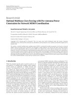
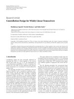
Figure 1: Two cellular systems with hexagonal cells and trisectorial
antennas at the base stations (reuse factor F
= 3, setting A, on the
right and F
= 7, setting B, on the left). The array is equipped with
N
= 4 antennas. Shaded sectors denote the allowed areas for user
and the three interferers belonging to the first ring of interference
(dashed lines identify the cell clusters of frequency reuse).

Δ
12
Δ
23
Δ
N
2
−1,
N
2
··· ···
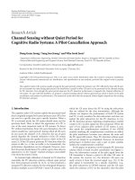
Figure 2: Nonuniform symmetric array structure for N even.
For illustration purposes, consider the interference sce-
narios sketched in Figure 1. Therein, we have two different
settings characterized by hexagonal cells and different reuse
factors (F
= 3 for setting A and F = 7 for setting B, frequency
reuse clusters are denoted by dashed lines). The base station
is equipped with a symmetric antenna array
1
containing an
even number N of directional antennas (N
= 4 in the exam-
ple) to cover an angular sector of 120 deg, other BS antenna
array design options are discussed in [8]. Each terminal is
provided with one omnidirectional antenna. On the consid-
ered radio resource (e.g., time-slot, frequency band, or or-
thogonal code), it is assumed there is only one active user in
the cell, as for TDMA, FDMA, or orthogonal CDMA. The
user of interest is located in the respective sector according

to the reuse scheme. The contribution of out-of-cell inter-
ferers is modelled as spatially correlated Gaussian noise. In
Figure 1, the first ring of interference is denoted by shaded
cells. The problem we tackle is that of finding the antenna
spacings in vector Δ
= [Δ
12
Δ
23
]
T
(as shown in the example)
1
The symmetric array assumption (as in the array structure of Figure 2)
has been made mainly for analytical convenience in order to simplify the
optimization problem. However, it is expected that for a scenario with a
symmetric layout of interference (such as setting A), the assumption of a
symmetric array does not imply any loss of optimality, while, on the other
hand, for an asymmetric layout (such as setting B), capacity gains could
be in principle obtained by deploying an asymmetric array.
so as to optimize given performance metrics, as detailed be-
low.
Two criteria are considered, namely, the minimization of
the average interference power at the output of a conven-
tional beamformer (matched filter) and the maximization
of the ergodic capacity (throughput). Since in many appli-
cations the position of users and interferers is not known
a priori at the time of the antenna deployment or the in-
cell/out-cell terminals are mobile, it is of interest to evaluate
the optimal spacings not only for a fixed position of users

and interferers but also by averaging the performance met-
ric over the positions of user and interferers within their cells
(see Section 2).
Even if the ergodic capacity criterion has to be considered
to be the most appropriate for array design in interference-
limited scenario, the interference power minimization is ana-
lytically tractable and highlights the justification for unequal
spacings. Therefore, the problem of minimizing the inter-
ference power is considered first and a closed-form expres-
sion for this criterion is derived as a function of the antenna
spacings (Section 4). This analysis allows to get insight into
the structure of the optimal array for different propagation
conditions and cellular layouts avoiding an extensive numer-
ical maximization of the ergodic capacity. The optimal ar-
ray deployments obtained according to the two criteria are
shown via numerical optimization to coincide for the con-
sidered scenarios (Section 5). More importantly, it is veri-
fied that substantial performance gain with respect to con-
ventionally designed linear antenna arrays (i.e., uniform λ/2
interelement spacing) can be harnessed by an optimized ar-
ray (up to 2.5 bit/s/Hz for the scenarios in Figure 1).
2. PROBLEM FORMULATION
The signal received by the N antenna array at the base station
serving the user of interest can be written as
y
= h
0
x
0
+

M

i=1
h
i
x
i
+ w,(1)
where h
0
is the N × 1 vector describing the channel gains
between the user and the N antennas of the base sta-
tion, x
0
is the signal transmitted by the user, h
i
and x
i
are
the corresponding quantities referred to the ith interferer
(i
= 1, ,M), w is the additive white Gaussian noise with
E[ww
H
] = σ
2
I. The channel vectors h
0
and {h
i

}
M
i
=1
are un-
correlated among each other and assumed to be zero-mean
complex Gaussian (Rayleigh fading) with spatial correlation
R
0
= E[h
0
h
H
0
]and{R
i
= E[h
i
h
H
i
]}
M
i
=1
,respectively.The
correlation matrices are obtained according to a widely em-
ployed geometrical model that assumes the scatterers as dis-
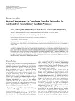
tributed along a ring around the terminal, see Figure 3. This
model was thoroughly studied in [2, 7]andabriefreview

can be found in Section 3. According to this model, the spa-
tial correlation matrices of the fading channel depend on
(1) the set of N/2 antenna spacings (N is even) Δ
=
[Δ
12
Δ
23
··· Δ
N/2, N/2+1
]
T
,whereΔ
ij
is the distance
between the ith and the jth element of the array (the
S. Savazzi et al. 3
Φ
0
φ
θ
0
θ
i
Φ
i
d
i
p
q

Δ
pq
d
0
r
0
r
i
Interferer
User
Figure 3: Propagation model for user and interferers: the scatterers
are distributed on a rings of radii r
i
around the terminals.
array is assumed to be symmetric as shown in Figure 2,
extension to an odd number of antennas N is straight-
forward);
(2) the relative positions of user and interferers with re-
spect to the base station of interest (these latter pa-
rameters can be conveniently collected into the vector
η
= [η
T
0
η
T
1
··· η
T
M

]
T
, where, as detailed in Figure 3,
vector η
0
= [d
0
θ
0
]
T
parametrizes the geometrical lo-
cation of the in-cell user and vectors η
i
= [d
i
θ
i
]
T
(i =
1, , M) describe the location of the interferers (i =
1, , M));
(3) the propagation environment is described by the angu-
lar spread of the scattered signal received by the base
station (φ
0
for the user and φ
i
(i = 1, , M) for the

interferers); notice that for ideally φ
i
→ 0allscatter-
ers come from a unique direction so that line-of-sight
(LOS) channel can be considered. Shadowing can be
possibly modelled as well, see Section 3 for further dis-
cussion.
2.1. Interference power minimization
From (1), the instantaneous total interference power at the
output of a conventional beamforming (matched filter) is [9]
P

h
0
, Δ, η

=
h
H
0
Qh
0
,(2)
where
Q
= Q

Δ, η
1
, , η

M

=
M

i=1
R
i

Δ, η
i

+ σ
2
I
N
(3)
accounts for the spatial correlation matrix of the interferers
and for thermal noise with power σ
2
. Notice that, for clar-
ity of notation, we explicitly highlighted that the interfer-
ence correlation matrices depend on the terminals’ locations
η and the antenna spacings Δ through nonlinear relation-
ships. The first problem we tackle is that of finding the set of
optimal spacings

Δ that minimizes the average (with respect
to fading) interference power, P (Δ, η)
= E

h
0
[P (h
0
, Δ, η)],
that is,
(Problem-1) :

Δ = arg min
Δ
P (Δ, η)(4)
for a fixed given position η of user and interferers. Problem
1 is relevant for fixed system with a known layout at the time
of antenna deployment. Moreover, its solution will bring in-
sight into the structure of the optimal array, which can be to
some extent generalized to a mobile scenario. In fact, in mo-
bile systems or in case the position of users and interferers is
not known a priori at the time of the antenna deployment,
it is more meaningful to minimize the average interference
power for any arbitrary position of in-cell user (η
0
)andout-
of-cells interferers (η
1
, η
2
, , η
M
). Denoting the averaging
operation with respect to users and interferers positions by

E
η
[P (Δ, η)], the second problem (9) can be can be stated as
(Problem-2) :

Δ = arg min
Δ
E
η

P (Δ, η)

. (5)
2.2. Ergodic capacity maximization
The instantaneous capacity for the link between the user and
the BS reads [2]
C

h
0
, Δ, η

=
log
2

1+h
H
0
Q

−1
h
0

[ bit/s/Hz], (6)
and depends on both the antenna spacings Δ and the termi-
nals’ locations η. For fast-varying fading channels (compared
to the length of the coded packet) or for delay-insensitive
applications, the performance of the system from an infor-
mation theoretic standpoint is ruled by the ergodic capacity
C(Δ, η). The latter is defined as the ensemble average of the
instantaneous capacity over the fading distribution,
C

Δ, η

= E
h
0

C

h
0
, Δ, η

. (7)
According to the alternative performance criterion herein
proposed, the first problem (4)isrecastedas
(Problem 1) :


Δ = arg max
Δ
C(Δ, η), (8)
and therefore requires the maximization of the ergodic ca-
pacity for a fixed given position η of user and interferers.
As before, denoting the averaging operation with respect to
users and interferers positions by E
η
[C(Δ, η)], the second
problem (5) can be modified accordingly:
(Problem 2) :

Δ = arg max
Δ
E
η

C(Δ, η)

. (9)
Different from the interference power minimization ap-
proach, in this case, functional dependence of the perfor-
mance criterion (7) on the antenna spacings Δ is highly non-
linear (see Section 3 for further details) and complicated by
the presence of the inverse matrix Q
−1
that relies upon Δ and
η. This implies both a large-computational complexity for
4 EURASIP Journal on Wireless Communications and Networking

0
0.5
1
1.5
2
2.5
3
3.5
4
4.5
5
40.5
45
36
31.5
27
22.5
Δ
12
λ
SIR
r2
(dB)
Δ
23
λ
00.511.52 2.53 3.544.55
(a)
0
0.5

1
1.5
2
2.5
3
3.5
4
4.5
5
16
17
15
13
12
11
14
Δ
12
λ
Ergodic capacity (bps/Hz)
Δ
23
λ
00.511.522.53 3.544.55
(b)
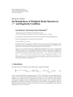
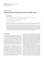
Figure 4: Setting-A: rank-2 approximation of the signal-to-interference ratio SIR
r2
(Δ, η)(23)versusΔ
12
/λ and Δ

23
/λ (a) compared with
ergodic capacity C(Δ,
η)(b)(r = 50 m). Circles denote optimal solutions.
the numerical optimization of (8)and(9), and the impossi-
bility to get analytical insight into the properties of the op-
timal solution. When the number of antenna array is suffi-
ciently small (as in Section 5), optimization can be reason-
ably dealt with through an extensive search over the opti-
mization domain and without the aid of any sophisticated
numerical algorithm. On the contrary, in case of an array
with a larger number of antenna elements, more efficient op-
timization techniques (e.g., simulated annealing) may be em-
ployed to reduce the number of spacings to be explored and
thus simplify the optimization process. Below we will prove
(by numerical simulations) that the limitations of the above
optimization (8)-(9) are mitigated by the criteria (4)-(5)still
preserving the final result.
3. SPATIAL CORRELATION MODEL
We consider a propagation scenario where each terminal, be
it the user or an interferer, is locally surrounded by a large
number of scatterers. The signals radiated by different scat-
terers add independently at the receiving antennas. The scat-
terers are distributed on a ring of radius r
0
around the ter-
minal (r
i
, i = 1, , M for the interferers) and the resulting
angular spread of the received signal at the base station is de-

noted by φ
0
 r
0
/d
0
(or φ
i
 r
i
/d
i
), as in Figure 3.Because
of the finite angular spreads
{φ
i
}
M
i
=0
, the propagation model
appears to be well suited for outdoor channels.
In [7], the spatial correlation matrix of the resulting
Rayleigh distributed fading process at the base station is com-
puted by assuming a parametric distribution of the scatterers
along the ring, namely, the von Mises distribution (variable
0
≤ ϑ<2π runs over the ring, see Figure 3):
f (ϑ)
=

1
2πI
0
(κ)
exp

κ cos(ϑ)

. (10)
By varying parameter κ, the distribution of the scatterers
ranges from uniform ( f (ϑ)
= 1/(2π)forκ = 0) to a Dirac
delta around the main direction of the cluster ϑ
= 0(for
κ
→∞). Therefore, by appropriately adjusting parameter κ
and the angular spreads for each user and interferers φ
i
,a
propagation environment with a strong line-of-sight com-
ponent (φ
i
 0 and/or κ →∞) or richer scattering (larger
φ
i
with κ small enough) can be modelled. The (normal-
ized) spatial correlation matrix has the general expression
for both user and interferers (for the (p, q)th element with
p, q
= 1, , N and i = 0, 1, , M)[7]:


R
i

θ
i
, Δ

pq
= exp

j
2π
λ
Δ
pq
sin

θ
i


·
I
0


κ
2
−


2π/λ

Δ
pq
φ
i
cos

θ
i

2

I
0
(κ)
.
(11)
It is worth mentioning that spatial channel models based on
different geometries such as elliptical or disk models [10, 11]
may be considered as well by appropriately modifying the
spatial correlation (11). Effects of mutual coupling (not ad-
dressed in this paper) between the array elements may be in-
cluded in our framework too, see [12, 13].
From (11), the spatial correlation matrices R
i
of the user
and interferers can be written as
R

i

η
i
, Δ

=
ρ
i
R
i

θ
i
, Δ

with ρ
i
=
K
d
α
i
, (12)
where K is an appropriate constant that accounts for receiv-
ing and transmitting antenna gain and the carrier frequency,
and α is the path loss exponent. The contribution of shad-
owing in (12) will be considered in Section 5.3 as part of an
additional log-normal random scaling term.
S. Savazzi et al. 5

0
0.5
1
1.5
2
2.5
3
3.5
4
4.5
5
26.5
27
26
25.5
25
24.5
24
23.5
23
22.5
Δ
12
λ
SIR
r1
(dB)
Δ
23
λ

00.511.522.533.544.55
(a)
0
0.5
1
1.5
2
2.5
3
3.5
4
4.5
5
12
12.5
11.5
11
10.5
Δ
12
λ
Ergodic capacity (bps/Hz)
Δ
23
λ
00.51.522.533.544.551
(b)
Figure 5: Setting-A: rank-1 approximation (a) of the signal-to-interference ratio, SIR
r1
(Δ, η), versus Δ

12
/λ and Δ
23
/λ. Dashed lines denote
the optimality conditions (24) obtained by the rank-1 approximation. As a reference, ergodic capacity is shown (b), for an angular spread
approaching zero.
4. REDUCED-RANK APPROXIMATION FOR
THE INTERFERENCE POWER
According to a reduced-rank approximation for the spa-
tial correlation matrices of user and interferers R
i
for i =
0, 1, , M, in this section, we derive an analytical closed
form expression for the interference power (2) to ease the
optimization of the antenna spacings Δ.InSection 4.1,we
consider the case where the angular spread for users and in-
terferers φ
i
is small so that a rank-1 approximation of the spa-
tial correlation matrices can be used. This first case describes
line-of-sight channels. Generalization to channel with richer
scattering is given in Section 4.2.
4.1. Rank-1 approximation (line-of-sight channels)
If the angular spread is small for both user and inter-
ferers
2
(i.e., φ
i
 1fori = 0, 1, , M), the asso-
ciated spatial correlation matrices

{R
i
}
M
i
=0
,canbecon-
veniently approximated by enforcing a rank-1 constraint.
For φ
i
 1, the following simplification holds in (11):
I
0
(

κ
2
− ((2π/λ)Δ
pq
φ
i
cos(θ
i
))
2
)/I
0
(κ)  1. Therefore, the
spatial correlation matrices (12) can be approximated as (we
drop the functional dependency for simplicity of notation)

R
i
 ρ · v
i
v
H
i
, (13)
2
Rank-1 approximation for the out-of-cell interferers is quite accurate
when considering large reuse factors as the angular spread experienced
by the array is reduced by the increased distance of the out-of-cell inter-
ferers.
where
v
i
(Δ, j) =

1exp

− jω

θ
i

Δ
12

··· exp


− jω

θ
i

Δ
1N


T
(14)
and ω
i
(θ) = 2π/λsin(θ
i
).
From (13), the channel vectors for user and interfer-
ers can be written as h
i
= γ
√
ρ
i
v
i
,whereγ ∼ CN (0, 1).
Therefore, within the rank-1 approximation, the interference
power reads (the additive noise contribution σ
2
I

N
has been
dropped since it is immaterial for the optimization problem)
P
1
(Δ, η) = v
H
0

M

i=1
ρ
i
v
i
v
H
i

v
0
, (15)
therefore, optimal spacings with respect to Problem 1 (4)can
be written as

Δ = arg min
Δ
P
1

(Δ, η), (16)
where the subscript is a reminder of the rank-1 approxima-
tion. The advantage of the rank-1 performance criterion (15)
is that it allows to derive an explicit expression as a function
of the parameters of interest. In particular, after tedious but
straightforward algebra, we get
P
1
(Δ, η)
=
M

i=1

ρ
i
N + ρ
i
L

j=1
4S

l
j
, θ
0
, θ
i


+ ρ
i
C

k=1
2S

c
k
, θ
0
, θ
i


,
(17)
6 EURASIP Journal on Wireless Communications and Networking
0
0.5
1
1.5
2
2.5
3
3.5
4
4.5
5
51

48
45
42
39
36
Δ
12
λ
SIR
r2
(dB)
Δ
23
λ
00.51 1.522.533.544.55
(a)
0
0.5
1
1.5
2
2.5
3
3.5
4
4.5
5
19
18
16

15
14
13
17
Δ
12
λ
Ergodic capacity (bps/Hz)
Δ
23
λ
00.511.52 2.533.544.55
(b)
Figure 6: Setting B: rank-2 approximation of the signal-to-interference ratio, SIR
r2
(Δ, η), (23)versusΔ
12
/λ and Δ
23
/λ (a) compared with
ergodic capacity C(Δ,
η)(b)(r = 50 m). Circles denote optimal solutions.
where S(x, θ
n
, θ
m
) = cos[2πx(sin(θ
n
)−sin(θ
m

))], L =

N
2

−
N/2

/2 is the number of “lateral spacings” l
i
= Δ
i,j
for
i
= 1, , N/2 −1, j = i+1, ,N −i, C = N/2 is the number
of “central spacings” c
i
= Δ
i,N−i
for i = 1, , N/2.
As a remark, notice that if there exists a set of antenna
spacing

Δ such that the user vector v
0
is orthogonal to the M
interference vectors
{v
i
}

M
i
=1
, then this nulls the interference
power, P
1
(Δ, η) = 0, and thus implies that

Δ is a solution to
(16) (and therefore to (4)).
4.2. Rank-a (a>1) approximation
In a richer scattering environment, the conditions on the an-
gular spread φ
i
 1 that justify the use of rank-1 approx-
imation can not be considered to hold. Therefore, a rank-a
approximation with a>1 should be employed (in general)
for the spatial correlation matrix of both user and interferers:
R
i

a

k=1
ρ
(k)
i
· v
(k)
i

v
(k)H
i
(18)
for i
= 0, 1, , M. The set of vectors {v
(k)
i
}
a
k
=1
in (18)isre-
quired to be linearly independent. In this paper, we limit the
analysis to the case a
= 2, which will be shown in Section 5
to account for a wide range of practical environments. The
expression of vectors v
(k)
i
from (11) with respect to the an-
tenna spacings is not trivial as for the rank-1 case. However,
in analogy with (14), we could set
v
(k)
i
=

1exp


−
jω
(k)
i
Δ
12

···
exp

−
jω
(k)
i
Δ
1N

T
,
(19)
where the wavenumbers ω
i
= [ω
(1)
i
, ω
(2)
i
] for user and inter-
ferers have to be determined according to different criteria.

In order to be consistent with the rank-1 case considered in
the previous section, here we minimize the Frobenius norm
of approximation error matrix
R
i
−

a
k=1
ρ
(k)
i
· v
(k)
i
v
(k)H
i

2
with respect to ω = [ω
(1)
i
, ω
(2)
i
]vectorandρ = [ρ
(1)
i
, ρ

(2)
i
]
vectors. For instance, for a uniform distribution of the scat-
terers along the ring (i.e., κ
= 0), it can be easily proved that
the optimal rank-2 approximation (for i
= 0, , M) results
in
ω
(1)
i
= ω
i

θ
i

+ ϕ
i
, ω
(2)
i
= ω
i

θ
i

−

ϕ
i
, (20)
where ϕ
i
= 2π/λ ·φ
i
cos(θ
i
)andρ
(1)
i
= ρ
(2)
i
= ρ
i
/2.
As for the rank-1 case in (17), after some alge-
braic manipulations, the performance criterion P
2
(Δ, η) =
E
h
0
[h
H
0
Qh
0

] admits an explicit expression in terms of the pa-
rameters of interest:
P
2
(Δ, η) =
M

i=1

ρ
i
N + ρ
i
L

j=1
4S

l
j
, θ
0
, θ
i

·
T
i

l

j

+ ρ
i
C

k=1
2S

c
k
, θ
0
, θ
i

T
i

c
k


,
(21)
where T
i
(x) = cos(ϕ
0
x)cos(ϕ

i
x); notice that in practical
environments, the angular spread for the in-cell user, ϕ
0
,
is larger than the out-of-cell interferers angular spreads,
ϕ
1
, , ϕ
M
(see Section 5). Therefore, the optimization prob-
lem (4) can be stated as

Δ = arg min
Δ
P
2
(Δ, η). (22)
5. NUMERICAL RESULTS
In this section, numerical results related to the layouts in
Figure 1 (N
= 4, M = 3, F = 3 for setting A and F = 7
for setting B with a cell diameter 
= 2 km) are presented.
Both the interference power minimization problems (4), (5)
S. Savazzi et al. 7
0
0.5
1
1.5

2
2.5
3
3.5
4
4.5
5
50
47
44
41
38
35
32
29
26
Δ
12
λ
SIR
r1
(dB)
Δ
23
λ
00.511.522.533.544.55
(a)
0
0.5
1

1.5
2
2.5
3
3.5
4
4.5
5
18
17
16
15
14
13
12
Δ
12
λ
Ergodic capacity (bps/Hz)
Δ
23
λ
00.51 1.522.533.544.55
(b)
Figure 7: Setting-B: rank-1 approximation (a) of the signal-to-interference ratio SIR
r1
(Δ, η)versusΔ
12
/λ and Δ
23

/λ. Circular marker de-
notes the optimal solution (24) obtained by the rank-1 approximation. As a reference, ergodic capacity is shown (b), for an angular spread
approaching zero.
and the ergodic capacity optimization problems (8), (9)for
Problems 1 and 2, respectively, are considered and com-
pared for various propagation environments. For Problem
1, user and interferers are located at the center of their re-
spective allowed sectors (
η,asinFigure 1), instead, for Prob-
lem 2 average system performances are computed over the al-
lowed positions (herein uniformly distributed) of users and
interferers.
Exploiting the rank-a-based approximation (rank-1 and
rank-2 approximations in (17)and(21), resp.), the inter-
ference power (for fixed user and interferers position
η as
for Problem 1, or averaged over terminal positions as for
Problem 2) is minimized with respect to the array spac-
ings and the resulting optimal solutions are compared to
those obtained through maximization of ergodic capacity.
Herein, we show that the proposed approach based on in-
terference power minimization is reliable in evaluating the
optimal spacings that also maximize the ergodic capacity
of the system. Since the number of antenna array is lim-
ited to N
= 4, ergodic capacity optimization can be car-
ried out through an extensive search over the optimization
domain.
The channels of user and interferers are assumed to be
characterized by the same scatterer radius r

i
= r (for the
rank-2 case) and r
→ 0 (for the rank-1 case) with κ = 0.
Furthermore, the path loss exponent is α
= 3.5. The signal-
to-background noise ratio (for the ergodic capacity simu-
lations) is set to Nρ
0
/σ
2
= 20 dB. For the sake of visual-
ization, the rank-a approximation of the interference power
is visualized (in dB scale) as the signal-to-interference ratio
(SIR):
SIR
ra
(Δ, η) =

ρ
0
P
a
(Δ, η)

dB
. (23)
5.1. Setting A (F
= 3)
Assuming at first fixed position

η for user and interfer-
ers (Problem 1), Figure 4(b) shows the exact ergodic capac-
ity C(Δ,
η)forr = 50 m (and thus the angular spread is
φ
0
= 5.75 deg, φ
1
= φ
3
= 0.87 deg, φ
2
= 0.82 deg) and
Figure 4(a) shows the rank-2 SIR approximation SIR
r2
(Δ, η)
(23)versusΔ
12
and Δ
23
for setting A. According to both op-
timization criteria, the optimal array has external spacing

Δ
12
 1.26 λ and internal spacing

Δ
23
 3.6 λ. It is interesting

to compare this result with the case of a line-of-sight channel
that is shown in Figure 5. In this latter scenario, the optimal
spacings are easily found by solving the rank-1 approximate
problem (16)as(k
= 0, 1, )

Δ
12
= (2k +1)Ψ

θ
1

with any

Δ
23
≥ 0 (24a)
or

Δ
12
+

Δ
23
= (2k +1)Ψ

θ
1


, (24b)
where Ψ(θ
1
) = λ/(2 sin(θ
1
))  0.6 λ as θ
1
= θ
2
= 52 deg.
Conditions (24) guarantee that the channel vector of the user
is orthogonal to the channel vectors of the first and third in-
terferers (the second is aligned so that mitigation of its inter-
ference is not feasible). Moreover, the optimal spacings for
the line-of-sight scenario (24)formagrid(seeFigure 5(a))
that contains the optimal spacings for the previous case in
Figure 4 with larger angular spread. Notice that, for every
practical purpose, the solutions to the ergodic capacity maxi-
mization (Figure 5(b)) are well approximated by SIR
r1
(Δ, η)
maximization in (23). As a remark, we might observe that
with line-of-sight channels, there is no advantage of deploy-
ing more than two antennas (

Δ
12
= 0or


Δ
23
= 0satisfy
the optimality conditions (24)) to exploit the interference
reduction capability of the array. Instead, for larger angu-
lar spread than the line-of-sight case, we can conclude that
8 EURASIP Journal on Wireless Communications and Networking
14.5
16
17.5
19
20.5
22
23.5
25
E
η
[SIR
r
2
](dB)
Δ
12
λ
=
Δ
23
λ
00.511.522.53 3.544.55
(a)

4
5.5
7
8.5
10
11.5
13
Ergodic capacity (bps/Hz)
Δ
12
λ
=
Δ
23
λ
00.511.522.53 3.544.55
(b)
Figure 8: Setting B: rank 2 approximation of the signal-to-interference ratio E
η
[SIR
r2
(Δ, η)] (a) and ergodic capacity E
η
[C(Δ, η)] (b) aver-
aged with respect to the position of user and interferers within the corresponding sectors for Δ
12
= Δ
23
.
(i)largeenoughspacingshavetobepreferredtoaccommo-

date diversity; (ii) contrary to the line-of-sight case, there is
great advantage of deploying more than two antennas (ap-
proximately 5-6 bit/s/Hz) whereas the benefits of deploying
more than three antennas are not as relevant (0.6 bit/s/Hz
for an optimally designed three-element array with uniform
spacing 3.6 λ); (iii) compared to the λ/2-uniformly spaced ar-
ray, optimizing the antenna spacings leads to a performance
gain of approximately 2.5 bit/s/Hz.
Let us now turn to the solution of Problem 2 (9). In this
case, the optimal set of spacings

Δ should guarantee the best
performance on average with respect to the positions of user
and interferers within the corresponding sectors. It turns out
that the optimal spacings are

Δ
12
=

Δ
23
 1.9 λ for both op-
timization criteria (not shown here), and the (average) per-
formance gain with respect to the conventional adaptive ar-
rays with

Δ
12
=


Δ
23
= λ/2 has decreased to approximately
0.5 bit/s/Hz. This conclusion is substantially different for sce-
nario B as discussed below.
5.2. Setting B (F
= 7)
For Problem 1, the exact ergodic capacity C(Δ,
η)forr =
50 m (and angular spread φ
0
= 5.75 deg, φ
1
= 0.34 deg,
φ
2
= 0.56 deg, and φ
3
= 0.58 deg) and the rank-2 approx-
imation SIR
r2
(Δ, η)(23) are shown versus Δ
12
and Δ
23
,in
Figure 6, for setting B. In this case, the optimal linear min-
imum length array consists, as obtained by both optimiza-
tion criteria, by uniform 2.2 λ spaced antennas. Optimal de-

sign of linear minimal length array leads to a 2.5 bit/s/Hz
capacity gain with respect to the capacity achieved through
an array provided with four uniformly λ/2 spaced antennas.
Similarly as before, we compare this result with the case of a
line-of-sight channel (Figure 7(a)), where the optimal spac-
ings, solution to the rank-1 approximate problem (16), are

Δ
12
= Ψ(θ
3
)  0.7 λ (external spacing) and

Δ
23
= 3Ψ(θ
3
) 
2.2 λ (internal spacing) θ
3
= 43.5 deg. In this case, the solu-
tions (confirmed by the ergodic capacity maximization, see
Figure 7(b)) guarantee that the channel vector of the user is
orthogonal to the channel vector of the third (predominant)
interferer (the second is almost aligned so that mitigation of
its interference is not feasible, the first one has a minor im-
pact on the overall performances). As pointed out before,
a larger angular spread than the line-of-sight case require-
larger spacings to exploit diversity.
As for Problem 2 (9), in Figure 8, we compare the ana-

lytical rank-2 approximation E
η
[SIR
r2
(Δ, η)] averaged over
the position of users and interferers with the exact aver-
aged ergodic capacity for a uniform-spaced antenna array.
The minimal length optimal solutions turn out again to be

Δ
12
=

Δ
23
 2.2 λ. Moreover, we can conclude that in this
interference layout the capacity gain with respect to the ca-
pacity achieved through an array provided with four uni-
formly λ/2 spaced antennas is 2.5 bit/s/Hz.
5.3. Impact of nonequal power interfering
due to shadowing effects
In this section, we investigate the impact of nonequal in-
terfering powers caused by shadowing on the optimal an-
tenna spacings. This amounts to include in the spatial cor-
relation model (12) a log-normal variable for both user and
interferers as ρ
i
= (K/d
i
α

) · 10
G
i
/10
and G
i
∼ N (0,σ
2
G
i
)for
i
= 0, 1, , M. All shadowing variables {G
i
}
M
i
=0
affect receiv-
ing power levels and are assumed to be independent. Figure 9
shows the ergodic capacity averaged over the shadowing pro-
cesses for setting B and r
= 50 m (as in Figure 6), when the
standard deviation of the fading processes are σ
G
0
= 3dBfor
the user (e.g., as for imperfect power control) and σ
G
i

= 8dB
(i
= 1, , M) for the interferers. By comparing Figure 9 with
S. Savazzi et al. 9
0
0.5
1
1.5
2
2.5
3
3.5
4
4.5
5
18
17
16
15
14
13
Δ
12
λ
Ergodic capacity (bps/Hz)
Δ
23
λ
00.511.522.533.544.55
Figure 9: Setting B: ergodic capacity C(Δ, η)averagedwithrespect

to the distribution of shadowing (r
= 50 m). Circle denotes the op-
timal solution.
Figure 6, we see that the overall effect of shadowing is that of
reducing the ergodic capacity but not to modify the optimal
antenna spacings; similar results can be attained by analyzing
the interference power (not shown here).
6. CONCLUSION
In this paper, we tackled the problem of optimal design of
linear arrays in a cellular systems under the assumption of
Gaussian interference. Two design problems are considered:
maximization of the ergodic capacity (through numerical
simulations) and minimization of the interference power at
the output of the matched filter (by developing a closed form
approximation of the performance criterion), for fixed and
variable positions of user and interferers. The optimal ar-
ray deployments obtained according to the two criteria are
shown via numerical optimization to coincide for the con-
sidered scenarios. The analysis has been validated by studying
two scenarios modelling cellular systems with different reuse
factors. It is concluded that the advantages of an optimized
antenna array as compared to a standard design depend on
both the interference layout (i.e., reuse factor) and the prop-
agation environment. For instance, for an hexagonal cellular
system with reuse factor 7, the gain can be on average as high
as 2.5 bit/s/Hz. As a final remark, it should be highlighted
that optimizing the antenna array spacings in such a way to
improve the quality of communication (by minimizing the
interference power) may render the antenna array unsuitable
for other applications where some features of the propaga-

tion are of interest, such as localization of transmitters based
on the estimation of direction of arrivals.
REFERENCES
[1] J. H. Winters, J. Salz, and R. D. Gitlin, “The impact of antenna
diversity on the capacity of wireless communication systems,”
IEEE Transactions on Communications, vol. 42, no. 234, pp.
1740–1751, 1994.
[2] G. J. Foschini and M. J. Gans, “On limits of wireless commu-
nications in a fading environment when using multiple an-
tennas,” Wireless Personal Communications,vol.6,no.3,pp.
311–335, 1998.
[3] F. Rashid-Farrokhi, K. J. R. Liu, and L. Tassiulas, “Transmit
beamforming and power control for cellular wireless systems,”
IEEE Journal on Selected Areas in Communications, vol. 16,
no. 8, pp. 1437–1449, 1998.
[4] J. Saholos, “A solution of the general nonuniformly spaced an-
tenna array,” Proceedings of the IEEE, vol. 62, no. 9, pp. 1292–
1294, 1974.
[5] J W. Liang and A. J. Paulraj, “On optimizing base station an-
tenna array topology for coverage extension in cellular radio
networks,” in Proceedings of the IEEE 45th Vehicular Technology
Conference (VTC ’95), vol. 2, pp. 866–870, Chicago, Ill, USA,
July 1995.
[6] R. Jana and S. Dey, “3G wireless capacity optimization for
widely spaced antenna arrays,” IEEE Personal Communica-
tions, vol. 7, no. 6, pp. 32–35, 2000.
[7] A. Abdi and M. Kaveh, “A space-time correlation model for
multielement antenna systems in mobile fading channels,”
IEEE Journal on Selected Areas in Communications, vol. 20,
no. 3, pp. 550–560, 2002.

[8] P. Zetterberg, “On Base Station antenna array structures for
downlink capacity enhancement in cellular mobile radio,”
Tech. Rep. IR-S3-SB-9622, Department of Signals, Sensors
& Systems Signal Processing, Royal Institute of Technology,
Stockholm, Sweden, August 1996.
[9] H. L. Van Trees, Optimum Array Processing, Wiley-Intersci-
ence, New York, NY, USA, 2002.
[10] R. B. Ertel, P. Cardieri, K. W. Sowerby, T. S. Rappaport, and J.
H. Reed, “Overview of spatial channel models for antenna ar-
ray communication systems,” IEEE Personal Communications,
vol. 5, no. 1, pp. 10–22, 1998.
[11] T. Fulghum and K. Molnar, “The Jakes fading model incorpo-
rating angular spread for a disk of scatterers,” in Proceedings
of the 48th IEEE Vehicular Technology Conference (VTC ’98),
vol. 1, pp. 489–493, Ottawa, Ont, Canada, May 1998.
[12] I. Gupta and A. Ksienski, “Effect of mutual coupling on the
performance of adaptive arrays,” IEEE Transactions on Anten-
nas and Propagation, vol. 31, no. 5, pp. 785–791, 1983.
[13] N. Maleki, E. Karami, and M. Shiva, “Optimization of antenna
array structures in mobile handsets,” IEEE Transactions on Ve-
hicular Technology, vol. 54, no. 4, pp. 1346–1351, 2005.