Báo cáo hóa học: " Research Article An ML-Based Estimate and the Cramer-Rao Bound for Data-Aided Channel Estimation in KSP-OFDM" pdf

Hindawi Publishing Corporation
EURASIP Journal on Wireless Communications and Networking
Volume 2008, Article ID 186809, 9 pages
doi:10.1155/2008/186809
Research Article
An ML-Based Estimate and the Cramer-Rao Bound for
Data-Aided Channel Estimation in KSP-OFDM
Heidi Steendam, Marc Moeneclaey, and Herwig Bruneel
The Department of Telecommunications and Information Processing (TELIN), Ghent University,
Sint-Pietersnieuwstraat 41, 9000 Gent, Belgium
Correspondence should be addressed to Heidi Steendam,
Received 3 May 2007; Revised 22 August 2007; Accepted 28 September 2007
Recommended by Hikmet Sari
We consider the Cramer-Rao bound (CRB) for data-aided channel estimation for OFDM with known symbol padding (KSP-
OFDM). The pilot symbols used to estimate the channel are positioned not only in the guard interval but also on some of the
OFDM carriers, in order to improve the estimation accuracy for a given guard interval length. As the true CRB is very hard to eval-
uate, we derive an approximate analytical expression for the CRB, that is, the Gaussian CRB (GCRB), which is accurate for large
block sizes. This derivation involves an invertible linear transformation of the received samples, yielding an observation vector of
which a number of components are (nearly) independent of the unknown information-bearing data symbols. The low SNR limit
of the GCRB is obtained by ignoring the presence of the data symbols in the received signals. At high SNR, the GCRB is mainly
determined by the observations that are (nearly) independent of the data symbols; the additional information provided by the
other observations is negligible. Both SNR limits are inversely proportional to the SNR. The GCRB is essentially independent of
the FFT size and the used pilot sequence, and inversely proportional to the number of pilots. For a given number of pilot symbols,
the CRB slightly increases with the guard interval length. Further, a low complexity ML-based channel estimator is derived from
the observation subset that is (nearly) independent of the data symbols. Although this estimator exploits only a part of the ob-
servation, its mean-squared error (MSE) performance is close the CRB for a large range of SNR. However, at high SNR, the MSE
reaches an error floor caused by the residual presence of data symbols in the considered observation subset.
Copyright © 2008 Heidi Steendam et al. This is an open access article distributed under the Creative Commons Attribution
License, which permits unrestricted use, distribution, and reproduction in any medium, provided the original work is properly
cited.
1. INTRODUCTION

Multicarrier systems have received considerable attention for
high data rate communications [1] because of their robust-
ness to channel dispersion. To cope with channel disper-
sion, the multicarrier system inserts between blocks of data a
guard interval, with a length larger than the channel impulse
response. The most commonly used types of guard interval
are cyclic prefix, zero padding, and known symbol padding.
In cyclic prefix OFDM, the guard interval consists of a cyclic
extension of the data block whereas in zero-padding OFDM,
no signal is transmitted during the guard interval [2]. In
OFDM with known symbol padding, (KSP-OFDM), which
is considered in this paper, the guard interval consists of a
number of known samples [3–5]. One of the advantages of
KSP-OFDM as compared to CP-OFDM and ZP-OFDM is
its improved timing synchronization ability: in CP-OFDM
and ZP-OFDM, low complexity timing synchronization al-
gorithms like the Schmidl-Cox [6] algorithm, typically result
in an ambiguity of the timing estimate over the length of the
guard interval, whereas in KSP-OFDM, low complexity tim-
ing synchronization algorithms can be found avoiding this
ambiguity problem by properly selecting the samples of the
guard interval [7].
In KSP-OFDM, the known samples from the guard in-
terval can serve as pilot symbols to obtain a data-aided es-
timate of the channel. However, as the length of the guard
interval is typically small as compared to the FFT length (to
keep the efficiency of the multicarrier system as high as pos-
sible) the number of known samples is typically too small to
obtain an accurate channel estimate. To improve the channel
estimation accuracy, the number of pilot symbols must be

increased. This can be done by increasing the guard interval
length or by keeping the length of the guard interval constant
2 EURASIP Journal on Wireless Communications and Networking
and replacing in the data part of the signal some data carriers
by pilot carriers. As the former strategy results in a stronger
reduction of the OFDM system efficiency than the latter [8],
the latter strategy will be considered.
In this paper, we derive an approximative analytical ex-
pression for the Gaussian Cramer-Rao bound (GCRB) for
channel estimation when the pilot symbols are distributed
over the guard interval and pilot carriers. The paper is or-
ganized as follows. In Section 2, we describe the system and
determine the GCRB. Further, we derive a low complexity
ML-based estimate for the channel in Section 3.Numerical
results are given in Section 4 and the conclusions are drawn
in Section 5.
2. SYSTEM MODEL AND CRAMER-RAO BOUND
2.1. System model
In KSP-OFDM, the data symbols to be transmitted are
grouped into blocks of N symbols: the ith symbol block is
denoted a
i
= (a
i
(0), , a
i
(N − 1))
T
. As explained below, a
i

contains information-bearing data symbols and pilot sym-
bols. The symbols a
i
are then modulated on the OFDM carri-
ers using an N-point inverse FFT. The guard interval, consist-
ing of ν known samples, is inserted after each OFDM symbol
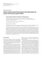
(this corresponds to the dark-gray area in Figure 1(a)), re-
sulting in N + ν time-domain samples s
i
during block i:
s
i
=

N
N + ν

F
+
a
i
b
g

,(1)
where F is the N
× N matrix corresponding to the FFT
operation, that is, F
k,
= (1/

√
N)e
−j2π(k/N)
,andb
g
=
(b
g
(0), , b
g
(ν − 1))
T
corresponds to the ν known samples
of the guard interval.
The sequence (1) is transmitted over a dispersive channel
with L taps h
= (h(0), , h(L − 1))
T
and disturbed by ad-
ditive white Gaussian noise w. The zero-mean noise compo-
nents w(k) have variance N
0
. To avoid interference between
symbols from neighboring blocks, we assume that the dura-
tion of the guard interval exceeds the duration of the channel
impulse length, that is, ν
≥ L − 1. Without loss of general-
ity, we consider the detection of the OFDM block with index
i
= 0, and drop the block index for notational convenience.

Taking the condition ν
≥ L −1 into account, the correspond-
ing N + ν received time-domain samples can be written as
r
= H
ch
s + w,(2)
where (H
ch
)
k,k

= h(k − k

) is the (N + ν) × (N + ν)chan-
nel matrix. For data detection, the known samples are first
subtracted from the received signal. Then, the ν samples of
the guard interval are added to the first ν samples of the data
part of the block, as shown in Figure 1(b), and an FFT is ap-
plied to the resulting N samples. As the known samples are
distorted by the channel (as can be seen in Figure 1(b)), the
channel needs to be known before the contribution from the
known samples can be removed from the received signal.
To estimate the channel, we assume that M pilot symbols
are available. As we select the length of the guard interval in
function of the channel impulse length and not in function
of the precision of the estimation, only ν of the M pilot sym-
bols can be placed in the guard interval. This implies that
M
− ν carriers in (1) must contain pilot symbols, which are

denoted by b
c
= (b
c
(0), , b
c
(M−ν−1))
T
.WedefineI
p
and
I
d
as the sets of carriers modulated by the pilot symbols and
the data symbols, respectively, with I
p
∪ I
d
={0, , N − 1}.
Hence, the symbol vector a contains M
− ν pilot symbols
b
c
and N + ν − M data symbols which are denoted by a
d
.
We assume that the data symbols are independent identically
distributed (i.i.d.) with E[
|a
d

(n)|
2
] = E
s
and the pilot sym-
bols are selected such that E[
|b
g
(m)|
2
] = E[|b
c
(n)|
2
] = E
s
.
The normalization factor

N/(N + ν)in(1) then gives rise
to E[
|s(m)|
2
] = E
s
. It can easily be verified that the obser-
vation of the N + ν time-domain samples corresponding to
one OFDM block (as shown in Figure 1(c)) contains suffi-
cient information to estimate h. Rewriting (2), we obtain
r

= Bh + w,(3)
where B
= B
g
+B
c
is a (N +ν)×L matrix. The matrix B
g
con-
tains the contributions from the pilot symbols in the guard
interval, and is given by

B
g

k,
=

N
N + ν
b
g

|k −  + ν|
N+ν

,(4)
where
|x|
K

is the modulo-K operation of x yielding a result
in the interval [0, K[, and b
g
(k) = 0fork ≥ ν.ThematrixB
c
consists of the contributions from the pilots transmitted on
the carriers, where
(B
c
)
k,
=

N
N + ν
s
p
(k − ). (5)
The vector s
p
equals the N-point IFFT of the pilot carriers
only, that is, s
p
= F
p
b
c
.TheN ×(M − ν)matrixF
p
consists

of a subset of columns of the IFFT matrix F
+
corresponding
to the set I
p
of pilot carriers. Note that s
p
(k) = 0fork<0or
k
≥ N. The disturbance in (3)canbewrittenas
w = HF
d
a
d
+ w = Hs
d
+ w,(6)
where H
k,
= h(k − )isa(N + ν) × N matrix. The N ×
(N + ν − M)matrixF
d
consists of a subset of columns of
F
+
corresponding to the set I
d
of data carriers. Hence, s
d
=

F
d
a
d
equals the N-point IFFT of the data carriers symbols
only, that is, the contribution from the data symbols to the
received time-domain samples r.
2.2. Gaussian Cramer-Rao bound
First, let us determine the Cramer-Rao bound of the estima-
tion of h from the observation r. The Cramer-Rao bound is
defined by R
h−

h
− J
−1
≥ 0[9], where R
h−

h
is the autocorre-
lation matrix of the estimation error h
−

h,

h is an estimate
of h, and the Fisher information matrix J is defined as
J
= E

r

∂
∂h
ln p(r
| h)

+

∂
∂h
ln p(r
| h)

. (7)
Heidi Steendam et al. 3
NT
νT
t
Block i
− 1Blocki +1Block i
(a) Transmitter
N samples to be processed
t
+
(b) Receiver
Observation interval
t
(c) Channel estimation
Figure 1: Time-domain signal of KSP-OFDM: (a) transmitted signal, (b) received signal and observation interval for data detection, and (c)

observation interval for channel estimation.
Hence, the MSE of an estimator is lower bounded by
E[h −

h
2
] = trace (R
h−

h
) ≥ trace (J
−1
). In our analysis,
we assume that s
d
= F
d
a
d
is zero-mean Gaussian distributed;
this yields a good approximation for large N + ν
−M (say for
large block sizes) and results in the Gaussian CRB (GCRB).
In this case, r given h is Gaussian distributed, that is, r
|
h∼N(Bh, R
w
), where R
w
= E

s
(N/(N +ν))HF
d
F
+
d
H
+
+N
0
I
N+ν
is the autocorrelation matrix of the disturbance w and I
K
is
the K
× K identity matrix. Hence, it follows that
ln p(r
| h) = C −
1
2
ln R
w
 − (r −Bh)
+
R
−1
w
(r − Bh),
(8)

where C is an irrelevant constant and R
w
 is the determi-
nant of R
w
. Note that as the autocorrelation matrix R
w
de-
pends on the channel taps h to be estimated, we need the
derivative of R
w
 and R
−1
w
with respect to h to obtain the
Fisher information matrix, and hence the GCRB. As in gen-
eral these derivatives are difficult to obtain, the computation
of the GCRB is in general very complex. In order to find an
analytical expression for the GCRB and avoid the difficulty
of finding the derivatives of R
w
 and R
−1
w
for a general auto-
correlation matrix R
w
, we suggest the following approach.
Let us consider the approximation of the data contri-
bution HF

d
a
d
in (6)by

F

Ha
d
, where the matrix

F
k,
=
(1/
√
N)e
j2π(kn

/N)
,

H is a diagonal matrix with diagonal el-
ements H
n

, n

∈ I
d

and
H
m
=
N−1

k=0
h(k)e
−j2π(km/N)
. (9)
In this approximation, we have neglected, in the contribu-
tion from a
d
to r, the transient at the edges of the received
block; this approximation is valid for long blocks, that is,
when N
 ν. When applying an invertible linear transfor-
mation that is independent of the parameter to be estimated,
to the observation r,thiswillhavenoeffect on the CRB.
Further, note that

Ha
d
contains only N + ν − M<N+ ν
components. Therefore, it is possible to find an invertible
linear transformation T that maps r to an (N + ν)
× 1vec-
tor r

= [r

T
1
r
T
2
]
T
,wherer
1
depends on the transmitted data
symbols a
d
and r
2
is independent of a
d
. This transform can
be found by performing the QR-decomposition of the ma-
trix

F, that is,

F = QV,whereQ is a (N + ν)×(N + ν) unitary
matrix Q
+
= Q
−1
and
V
=


U
0

, (10)
where U is an upper triangular matrix. Taking into account
that

F has dimension (N + ν) ×(N + ν −M), it follows that

F
(and thus V)hasrankN + ν
− M.Hence,V contains M zero
rows, that is, U is a (N + ν
− M) × (N + ν − M)matrixand
the all zero matrix 0 in (10) has dimension M
×(N + ν −M).
The transform matrix T is then given by T
= Q
+
, and the
resulting observations yield
r

= Tr =

r
1
r
2


=

B
1
B
2

h +

U
0


Ha
d
+

w
1
w
2

. (11)
In (11), B
1
and B
2
correspond to the first N+ν−M and last M
rows of TB, respectively. Because of the unitary nature of the

matrix T, the noise contributions w
1
and w
2
are statistically
independent and have the same mean and variance as the
noise w.
We now compute the GCRB related to the estimation of
the channel taps h based on the observation r

= Tr using
the approximation HF
d
=

F

H. The observation r

given h is
also Gaussian distributed, that is, r

| h∼N(TBh, R
w

), where
R
w

is the autocorrelation matrix of the disturbance w


= T w
and is given by
R
w
=

R
1
0
0R
2

, (12)
where R
1
= E
s
(N/(N + ν))U

H

H
+
U
+
+ N
0
I
N+ν−M

and R
2
=
N
0
I
M
.Asr
1
and r
2
given h are statistically independent, it can
easily be verified that the Fisher information matrix is given
by J
= J
1
+ J
2
,where
J
i
= E
r
i

∂
∂h
ln p

r

i
| h


+

∂
∂h
ln p

r
i
| h


(13)
with i
= 1, 2; and
ln p

r
i
| h

= C −
1
2
ln R
i
 −


r
i
− B
i
h

+
R
−1
i

r
i
− B
i
h

.
(14)
4 EURASIP Journal on Wireless Communications and Networking
We now compute the Fisher information matrices J
1
and J
2
, separately. First, we determine J
2
. As the observa-
tion r
2

= B
2
h + w
2
is independent of the data symbols, and
p(r
2
| h)∼N(B
2
h, N
0
I
M
), where B
2
is independent of h,it
can easily be found that
J
2
=
1
N
0
B
+
2
B
2
. (15)
Note that the CRB of an estimation can not increase by using

more observations. Hence, the GCRB obtained from the ob-
servation r
2
only is an upper bound for the GCRB obtained
from the whole observation r

.
Next, we determine J
1
, based on the observation r
1
=
B
1
h + U

Ha
d
+ w
1
only. Note that, although B
1
is indepen-
dent of h, the autocorrelation matrix R
1
of the disturbance
U

Ha
d

+ w
1
is not. Recall that to compute J
1
, we need the
derivative of R
1
 and (R
1
)
−1
with respect to h. These deriva-
tives can be written in an analytical form using the following
approximation: when M
−ν  N,

F

F
+
can be approximated
by the identity matrix I
N+ν−M
. When this assumption holds,
R
1
can be written as
R
1
= T

1

FΔ

F
+
T
+
1
, (16)
where T
1
consists of the N + ν −M first rows of T,andΔ is a
diagonal matrix with elements α

defined as
α

= N
0
+
N
N + ν
E
s


H
n




2
, n

∈ I
d
. (17)
Because

F has rank N+ν−M, T
1

F is a full-rank square matrix.
When A and B are square matrices, it follows that AB
=
AB.Hence,lnR
1
 reduces to
ln R
1
 = ln T
1

F

F
+
T
+

1
 +

n

∈I
d
ln

α


. (18)
Further, as T
1

F has full rank, the inverse of R
1
(16)caneasily
be computed:

R
1

−1
=


F
+

T
+
1

−1
Δ
−1

T
1

F

−1
. (19)
Using (18)and(19), the derivate of ln R
1
 and (R
1
)
−1
with
respect to h can easily be computed. Defining
γ
k,
=
N
N + ν
E
s

H
∗
n

e
−j2π(kn

/N)
,
β
k
=−
1
2

n

∈I
d
γ
k,
α

,
(20)
it follows after tedious but straightforward computations
(see the appendix) that the Fisher information matrix J
1
is
given by


J
1

k,k

=

B
+
1
R
−1
1
B
1

k,k

+ β
∗
k
β
k

+

n

∈I

d
γ
∗
k,
γ
k

,


α



2
. (21)
Combining (15)and(21), the total Fisher information
matrix, based on the observation of both r
1
and r
2
,isgiven
by (see the appendix)
(J)
k,k

=

B
+

R
−1
w
B

k,k

+ β
∗
k
β
k

+

n

∈I
d
γ
∗
k,
γ
k

,


α




2
. (22)
Let us now consider the behavior of the GCRB for low
and high values of E
s
/N
0
. When E
s
/N
0
 1, it follows from
(17), (20) that the second and third term in (22)arepropor-
tional to (E
s
/N
0
)
2
, whereas it can be verified from the defini-
tions of B and R
w
that the first term in (22) is proportional to
E
s
/N
0
. Hence, the first term in (22) is dominant at low E

s
/N
0
and the GCRB reduces to CRB = trace [(B
+
R
−1
w
B)
−1
]. Tak-
ing into account that at low E
s
/N
0
the autocorrelation matrix
R
w
reduces to N
0
I
N+ν
, the low SNR limit of the GCRB equals
trace (N
0
(B
+
B)
−1
), which is inversely proportional to E

s
/N
0
.
This low SNR limit equals the GCRB that results from ignor-
ing the data symbols a
d
in (6); this limit corresponds to the
low SNR limit of the true CRB that has been derived in [8].
To evaluate the low E
s
/N
0
limit of the (G)CRB, we approx-
imate B
+
B by its average over all possible pilot sequences,
that is, B
+
B = E[B
+
B]. We assume that the pilot symbols
are selected in a pseudorandom way. In that case, E[B
+
B]is
essentially equal to E[B
+
B] = E[B
+
g

B
g
]+E[B
+
c
B
c
]. The com-
ponents of the first term E[B
+
g
B
g
]aregivenby
E

B
+
g
B
g

k,k


=
N
N + ν
ν−1


=0
E

b
∗
g

| − k + ν|
N+ν

b
g



 − k

+ ν


N+ν

=
N
N + ν
ν−1

=0
E
s

δ
k,k

=
N
N + ν
νE
s
δ
k,k

.
(23)
The components of the second term E[B
+
c
B
c
]aregivenby
E

B
+
c
B
c

k,k



=
N
N + ν
N−1

=0
E

s
∗
p
( − k)s
p
( − k

))

=
N
N + ν
N−1

=0

m,m

∈I
p
1
N

E

b
∗
c
(m)b
c
(m

)

·
e
−j2π((−k)m/N)
e
j2π((−k

)m

/N)
=
N
N + ν
E
s
N
−1

=0


m∈I
p
1
N
e
j2π((k−k

)m/N)
≈
N
N + ν
(M
− ν)E
s
δ
k,k

.
(24)
When the pilot symbols are evenly distributed over the car-
riers (i.e., the set I
p
ofpilotcarriersisgivenbyI
p
={n
0
+
m
 | m = 0, ,M − ν − 1},wheren
0

belongs to the
set
{0, , ρ},withρ = (N − 1) − (M − ν − 1),  =
floor(N/(M − ν))) and M − ν divides N, the approxima-
tion in the last line in (24) turns into an equality. Taking
into account (23)and(24), E[B
+
B] can be approximated
by E[B
+
B] = (N/(N + ν))ME
s
I
L
, from which it follows
that the low E
s
/N
0
limit of the (G)CRB reduces to CRB =
(L/M)((N/(N + ν))(E
s
/N
0
))
−1
. Hence, the low E
s
/N
0

limit of
the (G)CRB is inversely proportional to the number of pilot
symbols M.
When E
s
/N
0
 1, it follows from (17), (20) that the sec-
ond and third term in (22) become independent of E
s
/N
0
.
Heidi Steendam et al. 5
Further, if we split the first term of (22)asB
+
R
−1
w
B =
B
+
1
R
−1
1
B
1
+(1/N
0

)B
+
2
B
2
(see the appendix), it can be ver-
ified from the definitions of B
1
, B
2
,andR
1
that the first
term B
+
1
R
−1
1
B
1
is independent of E
s
/N
0
and the second term
(1/N
0
)B
+

2
B
2
is proportional to E
s
/N
0
at high E
s
/N
0
.Hence,
the Fisher information matrix at high E
s
/N
0
is dominated
by the term (1/N
0
)B
+
2
B
2
so the high SNR limit of the GCRB
equals CRB
= trace [N
0
(B
+

2
B
2
)
−1
], which is inversely propor-
tional to E
s
/N
0
. This high SNR limit equals the GCRB corre-
sponding to J
−1
2
, which corresponds to exploiting for channel
estimation only the observations r
2
that are independent of
the data symbols. This indicates that at high SNR, the infor-
mation contained in the observations r
1
, that are affected by
the data symbols can be neglected as compared to the infor-
mation provided by r
2
. Based on this finding, we will derive
in Section 3 a channel estimator that only makes use of the
observations r
2
.

Finally, note that both the low and high E
s
/N
0
limits of
the GCRB are independent of h.
3. THE SUBSET ESTIMATOR
TheMLestimateofavectorh from an observation z is de-
fined as [9]:

h
ML
= arg max
h
p(z | h). (25)
In the previous section, we have found that all observations
were linear in the parameter h to be estimated: z
= Ah + ω,
where ω is zero-mean Gaussian distributed with autocorre-
lation matrix R
ω
.IfR
ω
is independent of h, the ML estimate
can easily be determined.
In the problem under investigation, the autocorrelation
matrix of the additive disturbance becomes independent of
h only for the observation r
2
. Based on the observation r

2
,
we can easily obtain the ML estimate of h:

h
ML
=

B
+
2
B
2

−1
B
+
2
r
2
. (26)
We call this the subset estimator, as only a subset of observa-
tions is used for the estimation. The mean-squared error of
thisestimateisgivenby
MSE
= E



h −


h
ML


2

=
trace

N
0

B
+
2
B
2

−1

. (27)
Hence, the MSE of this estimate reaches the subset GCRB
which equals trace (J
−1
2
), that is, the estimate is a minimum
variance unbiased (MVU) estimate. However, it should be
noted that (27) is valid under the assumption HF
d

=

F

H,
which for finite block sizes is only an approximation. For fi-
nite block sizes, the observation r
2
is affected by a residual
contribution from the data symbols. In that case, the MSE of
the estimate (26)isgivenby
MSE
= trace

DR
w
D
+

, (28)
where D
= (B
+
2
B
2
)
−1
B
+

2
T
2
and T
2
consists of the last M
rows of T. Note that the matrix D is proportional to (E
s
)
−1/2
.
At low E
s
/N
0
, the autocorrelation matrix R
w
converges to
N
0
I
N+ν
, in which case (28)convergesto(27), which is in-
versely proportional to E
s
/N
0
.AthighE
s
/N

0
, however, the
residual contribution of the data symbols will be domi-
nant, and the dominant part of R
w
that contributes to
(28) is proportional to E
s
.HenceathighE
s
/N
0
the MSE,
(28) will become independent of E
s
/N
0
: an error floor will
be present, corresponding to MSE
= trace (E
s
(N/(N +
ν))DHF
d
F
+
d
H
+
D

+
). Note that the subset estimate (26)isonly
a true ML estimate as long as the assumption HF
d
=

F

H is
valid; for finite block size, (26) is rather an ML-based ad hoc
estimate.
As the transform T is obtained by the QR-decomposition
of

F,and

F is known when the positions of the data sym-
bols are known, B
2
only depends on the known pilot symbols
and the known positions of the data carriers and the pilot
carriers. Hence, B
2
is known at the receiver and (B
+
2
B
2
)
−1

B
+
2
can be precomputed. Therefore, the estimate (26)canbeob-
tained with low complexity.
4. NUMERICAL RESULTS
In this section, we evaluate the GCRBs obtained from the
whole observation r
1
and r
2
(22) and the data-free obser-
vation r
2
only (15). Without loss of generality, we assume
the comb-type pilot arrangement [10] is used for the pilots
transmitted on the carriers. We assume that the pilots are
equally spaced over the carriers, that is, the positions of the
pilot carriers are I
p
={n
0
+m | m = 0, , M−ν−1},where
 = floor(N/(M − ν)) and n
0
belongs to the set {0, , ρ},
with ρ
= (N −1)−(M −ν−1). Note however that the results
can easily be extended for other types of pilot arrangements.
From the simulations we have carried out, we have found

that the equally spaced pilot assignment yields the best per-
formance results. Further, we assume an L-tap channel with
h()
= h(0)(L − ), for  = 0, , L − 1, which is normal-
ized such that

L−1

=0
|h()|
2
= 1; we have selected L = 8. The
pilot symbols are BPSK modulated and generated indepen-
dently from one block to the next. Unless stated otherwise,
we compute the GCRB and the MSE for a large number of
blocks and average over the blocks, in order to obtain results
that are independent of the selection of the pilot symbols.
In Figure 2, we show the normalized GCRB, defined as
CRB
= ((N/(N + ν))(E
s
/N
0
))
−1
NCRB, as a function of
the SNR
= E
s
/N

0
for the total observation (r
1
, r
2
) and the
subset r
2
of observations only. Further, the low SNR limit
trace (N
0
(B
+
B)
−1
) of the (G)CRB is shown. As expected, for
low SNR (<
−10 dB), the GCRB of the total observation co-
incides with the low SNR limit of the (G)CRB. At high SNR,
the GCRB reaches the GCRB (27) for the subset observa-
tion. Further, it can be observed that the low SNR limit of the
NCRB is essentially equal to L/M, as was shown in Section 2.
Note that the difference between the low SNR limit and the
high SNR limit is quite small (in our example the difference
amounts to about 10%); this indicates that most of the esti-
mation accuracy comes from the observation r
2
.
In Figure 3, the NCRB is shown as function of M for dif-
ferent values of the SNR. The (N)CRB is inversely propor-

tional to M for a wide range of M. At low and high values of
6 EURASIP Journal on Wireless Communications and Networking
M, the NCRB is increased as compared to L/M.Thiscanbe
explained by Figure 4, which shows the influence of the pilot
sequence on the GCRB. In this figure, the GCRB is computed
for 50 randomly generated pilot sequences. Further, the aver-
age of the GCRB over the random pilot sequences is shown.
Note that the GCRB depends on the values of the pilots
through the first term in (22)only.AthighvaluesofM, the
pilot spacing becomes
 = 2(forN/4 <M− ν <N/2 = 512)
and
 = 1(forM − ν >N/2 = 512); in that case pilots
are not evenly spread over the carriers but grouped in one
part of the spectrum, and the approximation in the last line
of (24) is no longer valid. This effect causes the peaks in the
curve at high M. The GCRB in this case clearly depends on
the values of the pilots: we observe an increase of the vari-
ance. The effect disappears when M
−ν is close to N/2 = 512
or N
= 1024: the spreading of the pilots over the spectrum
becomes again uniform. Also at low values of M, the aver-
age value of the GCRB and the variance of the GCRB are
increased. At low M, the contribution of the guard interval
pilots is dominant. From simulations, it follows that this con-
tribution strongly depends on the values of the pilots in the
guard interval, and has large outliers when the guard interval
pilots are badly chosen. Assuming the pilots in the guard in-
terval are B-PSK modulated, the lowest GCRB in this case

is achieved when the B-PSK pilots are alternating, that is,
b
g
={1,−1, 1, −1, }. When M increases, the relative im-
portance of the guard interval pilots reduces and the contri-
bution of the pilot carriers becomes dominant. The GCRB
turns out to be essentially independent of the values of the
pilot carriers, as these pilots are multiplied with complex ex-
ponentials, which have a randomizing effect on the contribu-
tions of the pilot carriers. Hence, for increasing M, the GCRB
becomes essentially independent of the used pilot sequence.
Figure 5 shows the dependency of the NCRB on the
guard interval length for a fixed total number of pilots. It
is observed that the NCRB slightly increases for increasing
guard interval length. This can be explained by noting that
when ν increases, the number of guard interval pilots in-
creases while the number of pilot carriers decreases. Hence,
when ν increases, the relative importance of the contribu-
tion of the guard interval pilots will increase. As shown in
Figure 4, this will cause an increase of the GCRB. Hence,
as the GCRB increases for increasing guard interval length
when the total number of pilots is fixed, it is better to keep
the guard interval length as small as possible (i.e., ν
= L − 1
in order to avoid intersymbol interference) and put the other
pilots on the carriers.
The dependency of the GCRB on the FFT size N is shown
in Figure 6. The GCRB is constant over a wide range of
N.OnlyatlowvaluesofN, the GCRB slightly increases.
Note that for low N, the approximations HF

d
=

F

H and

F

F
+
= I
N+ν−M
do not hold, and the approximate analytical
expression for the GCRB looses its practical meaning. How-
ever, for the range of N for which the derived approximation
for the GCRB is valid, we can conclude that the GCRB is in-
dependent of N. This can intuitively be explained as follows.
The FFT size N will mainly contribute to the GCRB through
the data symbols a
d
, as the number of data symbols increases
0.3
0.28
0.26
0.24
0.22
0.2
0.18
0.16

0.14
0.12
0.1
−50 −40 −30 −20 −10 0 10 20 30 40 50
E
s
/N
0
CRB
Subset CRB
Low SNR limit
L/M
NCRB
Figure 2: Normalized GCRB, ν = 7, N = 1024, M = 40.
1E +02
1E +01
1E +00
1E
− 01
1E
− 02
1E
− 03
1 10 100 1000
E
s
/N
0
= 0dB
E

s
/N
0
= 10 dB
E
s
/N
0
= 20 dB
L/M
M
NRCB
Figure 3: Influence of the number of pilots M on the GCRB, ν = 7,
N
= 1024.
1E +01
1E +00
1E
− 01
1E
− 02
1E −03
10 100 1000
E
s
/N
0
= 0dB
E
s

/N
0
= 10 dB
M
CRB
Simulation
Average
Figure 4: Influence of the pilot sequence on the GCRB, ν = 7, N =
1024.
Heidi Steendam et al. 7
010203040
E
s
/N
0
= 0dB
E
s
/N
0
= 10 dB
E
s
/N
0
= 20 dB
ν
NCRB
0
0.05

0.1
0.15
0.2
0.25
0.3
0.35
0.4
0.45
Figure 5: Influence of the guard interval length ν on the GCRB,
M
= 40, N = 1024.
1E +00
1E
− 01
1E
− 02
10 100 1000 10000
E
s
/N
0
= 0dB
E
s
/N
0
= 10 dB
N
CRB
Figure 6: Influence of the FFT length N on the GCRB, M = 40,

ν
= 7.
with increasing N. However, we have shown that most of the
estimation accuracy of the GCRB comes from the observa-
tion r
2
, which is the data-free part of the observation. There-
fore, the presence of the data symbols will have almost no
influence of the GCRB, resulting in the GCRB to be indepen-
dent of N.
In Figure 7, we show the GCRB for both the total obser-
vation and the subset observation, along with the low SNR
limit of the (G)CRB. Although it follows from Figure 2 that
the GCRB and the subset GCRB are larger than the low SNR
limit of the (G)CRB, the difference is small: the curves in
Figure 7 are close to each other. In Figure 7, we also show the
MSE (28) of the proposed subset estimator. As can be ob-
served, the MSE coincides with the subset GCRB for a large
range of SNR. Only for large SNR (>20 dB), the MSE shows
an error floor as shown in the previous section, indicating
that for E
s
/N
0
> 20 dB the approximation HF
d
=

F


H is no
longer valid. Further, we show in Figure 7 the MSE of a sub-
1E +05
1E +04
1E +03
1E +02
1E +01
1E +00
1E
− 01
1E
− 02
1E
− 03
1E
− 04
1E
− 05
1E
− 06
−50 −40 −30 −20 −10 0 10 20 30 40 50
E
s
/N
0
CRB
CRB
Subset CRB
Low SNR limit
MSE [8]

MSE subset
CRB, MSE M-ν
Figure 7: GCRB and MSE, N = 1024, M = 40, ν = 7.
optimal ML-based estimator for the channel, derived in [8]
and based on the estimator given in [11]. In the latter esti-
mator, it is assumed that the autocorrelation matrix R
w
of
the disturbance
w (6) is known. Assuming the autocorrela-
tion matrix R
w
does not depend on the parameters to be es-
timated (which is not the case), the latter estimator is derived
based on the ML estimation rule. It is clear that the estima-
tor proposed in this paper outperforms the estimator from
[8]. Further, in the latter estimator the autocorrelation ma-
trix R
w
is in general not known but must be estimated from
the received signal. Therefore, the complexity of the estima-
tor from [8] is much higher than that of the proposed esti-
mator, as in the former case, the autocorrelation matrix first
has to be estimated from the received signal before channel
estimation can be carried out.
5. CONCLUSIONS AND REMARKS
In this paper, we have derived an approximation (which is
accurate for large block size) for the Cramer Rao bound, that
is, the Gaussian Cramer-Rao bound, related to for data-aided
channel estimation in KSP-OFDM, when the pilot symbols

are distributed over the guard interval and pilot carriers. An
analytical expression for the GCRB is derived by applying
a suitable linear transformation to the received samples. It
turns out that the GCRB is essentially independent of the
FFT length, the guard interval, and the pilot sequence, and is
inversely proportional to the number of pilots and to E
s
/N
0
.
At low SNR, the GCRB obtained in this paper coincides with
the low SNR limit of the true CRB, derived in [8]. At high
SNR, the GCRB reaches the GCRB corresponding to the
data-independent subset of the observation, indicating that
at high SNR, observations affected by data symbols can be
safely ignored when estimating the channel. Further, we have
compared the MSE of the subset estimator with the obtained
GCRB and with the MSE of the ML-based channel estimator
from [8]. The proposed estimator coincides with the subset
8 EURASIP Journal on Wireless Communications and Networking
GCRB for a large range of SNR. Only at large SNR, the MSE
shows an error floor. However, the proposed estimator out-
performs the estimator from [8], both in terms of complexity
and performance.
In CP-OFDM, the N samples corresponding to the data
part of the received signal are transformed to the frequency
domain by an FFT, and the guard interval samples are not
transformed. In ZP-OFDM, first the samples from the guard
interval are added to the first ν samples from the data part
of the received signal, and then the N samples from the data

part are applied to an FFT, while the guard interval samples
are not transformed. In both cases, the used transform is an
invertible linear transformation that is independent of the
parameter to be estimated. As the different carriers do not in-
terfere with each other, it can be shown that the FFT outputs
corresponding to the pilot carriers contain necessary and suf-
ficient information to estimate the channel. Therefore, the
observations that are used to estimate the channel in CP-
OFDM and ZP-OFDM are the FFT outputs corresponding
to the pilot carriers; the observations corresponding to the
data carriers and the guard interval samples are neglected.
Hence, in CP-OFDM and ZP-OFDM channel estimation is
performed in the frequency domain. As the FFT outputs at
the pilot positions are independent of the transmitted data,
the ML channel estimate and associate true CRB for CP-
OFDM and ZP-OFDM are easily to obtain [8]. However,
in KSP-OFDM, such a simple linear transformation cannot
be found to obtain M observations independent from the
data symbols, that is, the pilots are split over the guard in-
terval and the carriers, and the data symbols interfere with
the guard interval carriers. Therefore, channel estimation in
KSP-OFDM is in general more complex than for CP-OFDM
and ZP-OFDM.
APPENDIX
A. DETERMINATION OF J
1
(21)
Taking into account (18)and(19), the derivative of ln p(r
1
|

h)withrespecttoh(k)isgivenby
dlnp(r
1
| h)
dh(k)
= β
k
− (r
1
− B
1
h)
+
R
−1
1
B
1
1
k
+(r
1
− B
1
h)
+

Q
k
(r

1
− B
1
h),
(A.1)
where

Q
k
=


F
+
T
+
1

−1
X
k

T
1

F

−1
,
X

k
= diag

γ
k,


α



2

;
(A.2)
1
k
is a vector of length L with a one in the kth position and
zeros elsewhere; and α

, γ
k,
,andβ
k
are defined as in (17),
(20). Hence, the elements of the Fisher information matrix
J
1
are given by


J
1

k,k

=

B
+
1
R
−1
1
B
1

k,k

+ β
∗
k
β
k

+ β
∗
k
trace



Q
k

R
1

+ β
k

trace


Q
+
k
R
1

+trace


Q
+
k
R
1

trace



Q
k

R
1

+trace


Q
+
k
R
1

Q
k

R
1

.
(A.3)
Taking into account that R
1
= T
1

FΔ


F
+
T
+
1
,

Q
k
=
(

F
+
T
+
1
)
−1
X
k
(T
1

F)
−1
and trace (XY) = trace (YX), it follows
that trace (

Q

k
R
1
) = trace (X
k
Δ)andtrace(

Q
+
k
R
1

Q
k

R
1
) =
trace (X
+
k
ΔX
k

Δ). Further, note that Δ = diag(α

), then it fol-
lows that
trace



Q
k
R
1

=−
2β
∗
k
(A.4)
and
trace


Q
+
k
R
1

Q
k

R
1

=


n

∈I
d
γ
∗
k,
γ
k

,


α



2
. (A.5)
Substituting (A.4)and(A.5)in(A.3)yields(21).
B. DETERMINATION OF J (22)
Substituting (21)and(15)inJ
= J
1
+ J
2
, it follows that the
Fisher information matrix J can be written as
J
k,k


=

B
+
1
R
−1
1
B
1

k,k

+
1
N
0

B
+
2
B
2

k,k

+ β
∗
k

β
k

+

n∈I
d
γ
∗
k,
γ
k

,


α



2
=

(TB)
+
R
−1
w

(TB)


k,k

+ β
∗
k
β
k

+

n∈I
d
γ
∗
k,
γ
k

,


α



2
,
(B.1)
where it was taken into account that

R
w

=

R
1
0
0R
2

,(B.2)
R
2
= N
0
I
M
,and
TB
=

B
1
B
2

. (B.3)
Further note that R
w


= TR
w
T
+
and the transform T is a
unitary matrix. Then it follows that the first term in (B.1)
can be rewritten as (TB)
+
R
−1
w

(TB) = B
+
R
−1
w
B, resulting in
(22).
REFERENCES
[1] J. A. C. Bingham, “Multicarrier modulation for data transmis-
sion: an idea whose time has come,” IEEE Communications
Magazine, vol. 28, no. 5, pp. 5–14, 1990.
[2] B. Muquet, Z. Wang, G. B. Giannakis, M. De Courville, and P.
Duhamel, “Cyclic prefixing or zero padding for wireless multi-
carrier transmissions?” IEEE Transactions on Communications,
vol. 50, no. 12, pp. 2136–2148, 2002.
Heidi Steendam et al. 9
[3] L. Deneire, B. Gyselinckx, and M. Engels, “Training sequence

versus cyclic prefix—a new look on single carrier communica-
tion,” IEEE Communications Letters, vol. 5, no. 7, pp. 292–294,
2001.
[4] R. Cendrillon and M. Moonen, “Efficient equalizers for single
and multicarrier environments with known symbol padding,”
in Proceedings of the 6th International Symposium on Signal
Processing and Its Applications (ISSPA ’01), vol. 2, pp. 607–610,
Kuala-Lampur, Malaysia, August 2001.
[5] O. Rousseaux, G. Leus, and M. Moonen, “A suboptimal itera-
tive method for modified maximum likelihood sequence esti-
mation in a multipath context,” EURASIP Journal on Applied
Signal Processing, vol. 2002, no. 12, pp. 1437–1447, 2002.
[6] T. M. Schmidl and D. C. Cox, “Robust frequency and timing
synchronization for OFDM,” IEEE Transactions on Communi-
cations, vol. 45, no. 12, pp. 1613–1621, 1997.
[7]U.MengaliandA.N.D’Andrea,Synchronization Techniques
for Digital Receivers, Plenum Press, New York, NY, USA, 1997.
[8] H. Steendam and M. Moeneclaey, “Different guard interval
techniques for OFDM: performance comparison,” in Proceed-
ings from the 6th International Workshop on Multi-Carrier
Spread Spectrum (MC-SS ’07), vol. 1, pp. 11–24, Herrsching,
Germany, May 2007.
[9] H.L.VanTrees,Detection, Estimation and Modulation Theor y,
John Wiley & Sons, New York, NY, USA, 1968.
[10] F. Tufvesson and T. Maseng, “Pilot assisted channel estima-
tion for OFDM in mobile cellular systems,” in Proceedings of
IEEE 47th Vehicular Technology Conference (VTC ’97), vol. 3,
pp. 1639–1643, Phoenix, Ariz, USA, May 1997.
[11] O. Rousseaux, G. Leus, and M. Moonen, “Estimation and
equalization of doubly selective channels using known sym-

bol padding,” IEEE Transactions on Sig nal Processing, vol. 54,
no. 3, pp. 979–990, 2006.