Báo cáo hóa học: " Research Article Dereverberation by Using Time-Variant Nature of Speech Production System" pptx

Hindawi Publishing Corporation
EURASIP Journal on Advances in Signal Processing
Volume 2007, Article ID 65698, 15 pages
doi:10.1155/2007/65698

Research Article
Dereverberation by Using Time-Variant Nature of
Speech Production System
Takuya Yoshioka, Takafumi Hikichi, and Masato Miyoshi
NTT Communication Science Laboratories, NTT Corporation 2-4, Hikaridai, Seika-cho, Soraku-gun, Kyoto 619-0237, Japan
Received 25 August 2006; Revised 7 February 2007; Accepted 21 June 2007
Recommended by Hugo Van hamme
This paper addresses the problem of blind speech dereverberation by inverse filtering of a room acoustic system. Since a speech
signal can be modeled as being generated by a speech production system driven by an innovations process, a reverberant signal is
the output of a composite system consisting of the speech production and room acoustic systems. Therefore, we need to extract
only the part corresponding to the room acoustic system (or its inverse filter) from the composite system (or its inverse filter). The
time-variant nature of the speech production system can be exploited for this purpose. In order to realize the time-variance-based
inverse filter estimation, we introduce a joint estimation of the inverse filters of both the time-invariant room acoustic and the
time-variant speech production systems, and present two estimation algorithms with distinct properties.
Copyright © 2007 Takuya Yoshioka et al. This is an open access article distributed under the Creative Commons Attribution
License, which permits unrestricted use, distribution, and reproduction in any medium, provided the original work is properly
cited.

1.

INTRODUCTION

Room reverberation degrades speech intelligibility or corrupts the characteristics inherent in speech. Hence, dereverberation, which recovers a clean speech signal from its reverberant version, is indispensable for a variety of speech processing applications. In many practical situations, only the
reverberant speech signal is accessible. Therefore, the dereverberation must be accomplished with blind processing.
Let an unknown signal transmission channel from a
source to possibly multiple microphones in a room be modeled by a linear time invariant system (to provide a unified

description independent of the number of microphones, we
refer to a set of signal transmission channel(s) from a source
to possibly multiple microphones as a signal transmission
channel. The channel from the source to each of the microphones is called a subchannel. A set of signal(s) observed by
the microphone(s) is refered to as an observed signal. We
also refer to an inverse filter set, which is composed of filters applied to the signal observed by each microphone, as
an inverse filter). The observed signal (reverberant signal)
is then the output of the system driven by the source signal
(clean speech signal). On the other hand, the source signal is
modeled as being generated by a time variant autoregressive
(AR) system corresponding to an articulatory filter driven by
an innovations process [1]. In what follows, for the sake of

definiteness, the AR system corresponding to the articulatory filter and the system corresponding to the room’s signal
transmission channel are refered to as the speech production
system and the room acoustic system, respectively. Then, the
observed signal is also the output of the composite system
of the speech production and room acoustic systems driven
by the innovations process. In order to estimate the source
signal, the dereverberation may require the inverse filter of
the room acoustic system. Therefore, blind speech dereverberation involves the estimation of the inverse filter of the
room acoustic system separately from that of the speech production system under the condition that neither the parameters of the speech production system nor those of the room
acoustic system are available.
Several approaches to this problem have already been investigated. One major approach is to exploit the diversity between multiple subchannels of the room acoustic system [2–
6]. This approach seems to be sensitive to order misdetection or additive noise since it strongly exploits the isomorphic relation between the subspace formed by the source signal and that formed by the observed signal. The so-called
prewhitening technique achieved some positive results [7–
10]. It relies on the heuristic knowledge that the characteristics of the low order (e.g., 10th order [8]) linear prediction
(LP) residue of the observed signal are largely composed of
those of the room acoustic system. Based on this knowledge,

2
this technique regards the residual signal generated by applying LP to the observed signal as the output of the room
acoustic system driven by the innovations process. Then, the
inverse filter of the room acoustic system can be obtained by
using methods designed for i.i.d. series. Although methods
incorporating this technique may be less sensitive to additive noise than the subspace approach, the dereverberation
performance remains insufficient since the heuristics is just a
crude approximation. Also methods that estimate the source
signal directly from the observed signal by exploiting features
inherent in speech such as harmonicity [11] or sparseness
[12] have been proposed. The source estimate is then used
as a reference signal when calculating the inverse filter of the
room acoustic system. However, the influence of source estimation errors on the inverse filter estimates remains to be
revealed, and a detailed investigation should be undertaken.
As an alternative to the above approach, the time variant
nature of the speech production system may help us to obtain the inverse filter of the room acoustic system separately
from that of the speech production system. Let us consider
the inverse filter of a composite system consisting of speech
production and room acoustic systems. The overall inverse
filter is composed of the inverse filters of the room acoustic
and speech production systems. The inverse filter of the room
acoustic system is time invariant while that of the speech production system is time variant. Hence, if it is possible to extract only the time invariant subfilter from the overall inverse
filter, we can obtain the inverse filter of the room acoustic system. This time-variance-based approach was first proposed
by Spencer and Rayner [13] in the context of the restoration of gramophone recordings. They implemented this approach simply; the overall inverse filter is first estimated, and
then, it is decomposed into time invariant and time variant
subfilters. However, it would be extremely difficult to obtain
an accurate estimate of the overall inverse filter, which has
both time invariant and time variant zeros especially when
the sum of the orders of both systems is large [14]. Therefore, the method proposed in [13] is inapplicable to a room

environment.
This paper proposes estimating both the time invariant
and time variant subfilters of the overall inverse filter directly
from the observed signal. The proposed approach skips the
estimation of the overall inverse filter, which is the drawback
of the conventional method. Let us consider filtering the observed signal with a time invariant filter and then with a time
variant filter. When the output signal is equalized with the
innovations process, the time invariant filter becomes the inverse filter of the room acoustic system whereas the time variant filter negates the speech production system. Thus, we can
obtain the inverse filter of the room acoustic system simply
by adjusting the parameters of the time invariant and time
variant filters so that the output signal is equalized with the
innovations process. We then propose two blind processing
algorithms based on this idea. One uses a criterion involving
the second-order statistics (SOS) of the output; the other utilizes the higher-order statistics (HOS). Since SOS estimation
demands a relatively small sample size, the SOS-based algorithm will be efficient in terms of the length of the observed
signals. On the other hand, the HOS-based algorithm will

EURASIP Journal on Advances in Signal Processing
provide highly accurate inverse filter estimates because the
HOS brings additional information. Performance comparisons revealed that the SOS-based algorithm improved the
rapid speech transmission index (RASTI), which is a measure
of speech intelligibility, from 0.77 to 0.87 by using observed
signals of at most five seconds. In contrast, the HOS-based algorithm estimated the inverse filters with a RASTI of nearly
one when observed signals of longer than 20 seconds were
available. The main variables used in this paper are listed in
Table 1 as a reference.
2.
2.1.

PROBLEM STATEMENT

Problem formulation

The problem of speech dereverberation is formulated as follows. Let a source signal (clean speech signal) be represented
by s(n), and the impulse response of an M × 1 linear finite impulse response (FIR) system (room acoustic system) of order
K by {h(k) = [h1 (k), . . . , hM (k)]T }0≤k≤K . Superscript T indicates the transposition of a vector or a matrix. An observed
signal (reverberant signal) x(n) = [x1 (n), . . . , xM (n)]T can be
modeled as
K

x(n) =

h(k)s(n − k).

(1)

k=0

Here, x(n) consists of M signals from the M microphones. By
using the transfer function of the room acoustic system, we
can rewrite (1) as
x(n) = H(z) s(n),
K

H(z) =

(2)
T

h(k)z−k = H1 (z), . . . , HM (z) ,

(3)

k=0

where [z−1 ] represents a backward shift operator. Hm (z) is
the transfer function of the subchannel of H(z), corresponding to the signal transmission channel from the source to
the mth microphone. Then, the task of dereverberation is
to recover the source signal from N samples of the observed signal. This is achieved by filtering the observed signal x(n) with the inverse filter of the room acoustic system
H(z). Let y(n) denote the recovered signal and let {g(k) =
[g1 (k), . . . , gM (k)]T }−∞≤k≤∞ be the impulse response of the
inverse filter. Then, y(n) is represented as
∞

g(k)T x(n − k),

y(n) =

(4)

k=∞

or equivalently,
y(n) = G(z)T x(n),
∞

G(z) =

g(k)z−k .

(5)

(6)

k=∞

Note that, by definition, the recovered signal y(n) is
a single signal. We want to set up the tap weights
{gm (k)}1≤m≤M, −∞≤k≤∞ of the inverse filter so that y(n) is


Takuya Yoshioka et al.

3
Table 1: List of main variables.

Variable
M
N
K
L
P
W
T
s(n)
x(n)
y(n)
e(n)
d(n)
h(k)
g(k)
b(k, n)

a(k, n)
H(z), and so on
GCD{P1 (z), . . . , Pn (z)}
H (ξ)
J(ξ)
I(ξ1 , . . . , ξn )
K(ξ1 , . . . , ξn )
υ(ξ)
κi (ξ)
Σ(ξ)

Description
Number of microphones
Number of samples
Order of room acoustic system
Order of inverse filter of room acoustic system
Order of speech production system
Size of window function
Number of time frames
Source signal
Possibly multichannel observed signal
Estimate of source signal
Innovations process
Estimate of innovations process
Impulse response of room acoustic system
Impulse response of inverse filter of room acoustic system
Parameter of speech production system
Estimate of parameter of speech production system
Transfer function of room acoustic system {h(k)}0≤k≤K , and so on
Greatest common divisor of polynomials P1 (z), . . . , Pn (z)

Differential entropy of possibly multivariate random variable ξ
Negentropy of possibly multivariate random variable ξ
Mutual information between random variables ξ1 , . . . , ξn
Correlatedness between random variables ξ1 , . . . , ξn
Variance of random variable ξ
ith-order cumulant of random variable ξ
Covariance matrix of multivariate random variable ξ

equalized with the source signal s(n) up to a constant scale
and delay. This requirement can also be stated as
G(z)T H(z) = αz−β ,

(7)

where α and β are constants representing the scale and delay
ambiguity, respectively.
Next, the model of the source signal s(n) is given as follows. A speech signal is widely modeled as being generated by
a nonstationary AR process [1]. In other words, the speech
signal is the output of a speech production system modeled
as a time variant AR system driven by an innovations process.
Let {b(k, n)}n∈Z, 1≤k≤P , where Z is the set of integers, denote
the time dependent parameters of the speech production system of order P and let e(n) denote the innovations process.
Then, s(n) is described as
P

s(n) =

b(k, n)s(n − k) + e(n),

(1) the innovations {e(n)}n∈Z consist of zero-mean independent random variables,

(2) the speech production system 1/(1 − B(z, n)) has no
time invariant pole. This assumption is equivalent to
the following equation:
GCD . . . , 1 − B(z, 0), 1 − B(z, 1), . . . = 1,

where GCD{P1 (z), . . . , Pn (z)} represents the greatest
common divisor of polynomials P1 (z), . . . , Pn (z).
Although assumption (1) does not hold for a voiced portion
of speech in a strict sense due to the periodic nature of vocal cord vibration, the assumption has been widely accepted
in many speech processing techniques including the linear
predictive coding of a speech signal. A comment on the validity of assumption (2) is provided in Section 4.
2.2.

or equivalently,
1
e(n),
1 − B(z, n)
P

B(z, n) =
k=1

b(k, n)z−k .

(11)

(8)

k=1

s(n) =

In this paper, we assume that

(9)
(10)

Fundamental problem

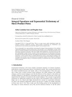
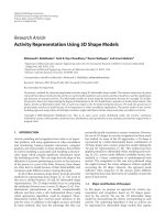
Figure 1 depicts the system that produces the observed signal
from the innovations process. We can see that the observed
signal is the output of H(z)/(1 − B(z, n)), which we call the
overall acoustic system, driven by the innovations process.
As mentioned above, our objective is to estimate the inverse filter of H(z). Despite this objective, we know only the
statistical property of the innovations process e(n), specified


4

EURASIP Journal on Advances in Signal Processing
Overall acoustic system
Speech production
system
(1-input 1-output)

e(n)
1

1
1 − B(z, n)

s(n)

Time-invariant
Time-variant
filter
filter
(M-input 1-output) (1-input 1-output)

Room acoustic
system
(1-input M-output)
x(n)

H(z)
1

e(n)

M

1

s(n)
x(n)
y(n)
1
1 − B(z, n) 1 H(z) M G(z) 1 1 − A(z, n) 1 d(n)
Room
Speech

acoustic
production
system
system
Overall acoustic system

Figure 1: Schematic diagram of system producing observed signal
from innovations process.

by assumption (1); neither the parameters of 1/(1 − B(z, n))
nor those of H(z) are available. Therefore, we face the critical problem of how to obtain the inverse filter of H(z) separately from that of 1/(1 − B(z, n)) with blind processing.
This is the cause of the so-called excessive whitening problem
[6], which indicates that applying methods designed for i.i.d.
series (e.g., see [15, 16] and references therein) to a speech
signal results in cancelling not only the characteristics of the
room acoustic system H(z) but also the average characteristics of the speech production system 1/(1 − B(z, n)).
3.

TIME-VARIANCE-BASED APPROACH

In order to overcome the problem mentioned above, we have
to exploit a characteristic that differs for the room acoustic system H(z) and the speech production system 1/(1 −
B(z, n)). We use the time variant nature of the speech production system as such a characteristic.
Let us consider the inverse filter of the overall acoustic
system H(z)/(1 − B(z, n)). Since the overall acoustic system
consists of a time variant part 1/(1 − B(z, n)) and a time invariant part H(z), the inverse filter accordingly has both time
invariant and time variant zeros. The set of time invariant zeros forms the inverse filter of the room acoustic system H(z)
while the time variant zeros constitute the inverse filter of
the speech production system 1/(1 − B(z, n)). Hence, we can
obtain the inverse filter of the room acoustic system by extracting the time invariant subfilter from the inverse filter of

the overall acoustic system.
3.1. Review of conventional methods
A method of implementing the time-variance-based inverse
filter estimation is proposed in [13, 17]. The method proposed in [13, 17] identifies the speech production system
and the room acoustic system assuming that both systems
are modeled as AR systems. The overall acoustic system is
first estimated from several contiguous disjoint observation
frames. In this step, it is assumed that the overall acoustic system is time invariant within each frame. Then, poles
commonly included in the framewise estimates of the overall acoustic system are collected to extract the time invariant
part of the overall acoustic system.

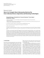
Figure 2: Schematic diagram of global system from innovations
process to its estimate.

The method imposes the following two conditions.
(i) The frame size is larger than the order of the room
acoustic system as well as that of the speech production system.
(ii) None of the system parameters change within a single
frame.
However, the parameters of the speech production system
change by tens of milliseconds while the order of the room
acoustic system may be equivalent to several hundred milliseconds. Therefore, we can never design a frame size that
meets those two conditions. This frame-size problem is discussed in more detail in Section 3.2.
Moreover, this method assumes that the room acoustic
system is minimum phase, which may be an unrealistic assumption. Therefore, it is difficult to apply this method to an
actual room environment.
Reference [14] proposes another method of implementing the time-variance-based inverse filter estimation. The
method estimates only the room acoustic system based on
maximum a posteriori estimation assuming that the innovations process e(n) is Gaussian white noise. However, the
method also assumes the room acoustic system to be minimum phase.

3.2.

Novel method based on joint estimation of time
invariant/time variant subfilters

The two requirements for the frame size with the conventional method arise from the fact that it estimates the overall
acoustic system in the first step. Therefore, we propose the
joint estimation of the time invariant and time variant subfilters of the inverse filter of the overall acoustic system directly
from the observed signal x(n).
Let us consider filtering x(n) with time invariant filter G(z) and then with time variant filter 1 − A(z, n) (see
Figure 2). If we represent the parameters of 1 − A(z, n) by
{a(k, n)}1≤k≤P , the final output d(n) is given as follows:

P

d(n) = y(n) −

a(k, n)y(n − k),
k=1

(12)


Takuya Yoshioka et al.

5

or equivalently,
d(n) = 1 − A(z, n) y(n),
P

A(z, n) =

−k

a(k, n)z ,

(13)
(14)

k=1

where y(n) is given by (5). Then, we have the following theorem under assumption (2).
Theorem 1. Assume that the final output signal d(n) is equalized with innovations process e(n) up to a constant scale and
delay, and that 1 − A(z, n) has no time invariant zero:
d(n) = αe(n − β),
GCD 1 − A(z, 1), . . . , 1 − A(z, N) = 1.

{d(n)}1≤n≤N satisfies assumption (1). In this section, we develop a criterion based only on the SOS of {d(n)}. To be more
precise, we try to uncorrelate {d(n)}.

We assume the following two conditions additionally in
this section.
(i) M ≥ 2, that is, we use multiple microphones.
(ii) Subchannel transfer functions H1 (z), . . . , HM (z) have
no common zero.
Under these assumptions, the observed signal x(n) is an AR
process driven by the source signal s(n) [16]. Therefore, we
can substitute an FIR inverse filter of order L for the doublyinfinite inverse filter in (4) as
L

(15)

Here, we can restrict the first tap of G(z) as
⎧
⎪1
⎨

m = 1,
gm (0) = ⎪
⎩0 m = 2, . . . , M,

Proof. The proof is given in Appendix A.
This theorem states that we simply have to set up the tap
weights {gm (k)}1 and {a(k, n)} so that d(n) is equalized with
αe(n − β). The calculated time invariant filter G(z) corresponds to the inverse filter of the room acoustic system H(z),
and the time variant filter 1 − A(z, n) corresponds to that of
the speech production system 1/(1 − B(z, n)). Thus, we can
conclude that the joint estimation of the time invariant/time
variant subfilters is a possible solution to the problem described in Section 2.2.
At this point, we can clearly explain the drawback of the
conventional method with a large frame size. When using a
large frame size, it is impossible to completely equalize d(n)
with αe(n − β) because 1/(1 − B(z, n)) varies within a single
frame. Hence, the estimate of the overall acoustic system in
each frame is inevitably contaminated by estimation errors.
These errors make it difficult to extract static poles from the
framewise estimates of the overall acoustic system. By contrast, the joint estimation that we propose does not involve
the estimation of the inverse filter of the overall acoustic system. Therefore, a frame size shorter than the order of the
room acoustic system can be employed, which enables us to

equalize d(n) with αe(n − β).
Since the innovations process e(n) is inaccessible in reality, we have to develop criteria defined solely by using d(n).
These criteria are provided in the next two sections. The algorithms derived can deal with a nonminimum phase system
as the room acoustic system since they use multiple microphones and/or the HOS of the output d(n) [15, 16].
ALGORITHM USING SECOND-ORDER STATISTICS

Since output signal d(n) is an estimate of innovations process
e(n), it would be natural to set up the tap weights {gm (k)}
and {a(k, n)} so that the statistical property of the outputs
1

Hereafter, we will omit the range of indices unless necessary.

(17)

k=0

(16)

Then, the time invariant filter G(z) satisfies (7).

4.

g(k)T x(n − k).

y(n) =

(18)

where the microphone with m = 1 is nearest to the source

(see [16] for details).
4.1.

Loss function

Let K(ξ1 , . . . , ξn ) denote a suitable measure of correlatedness
between random variables ξ1 , . . . , ξn . Then, the problem is
mathematically formulated as
minimize K d(1), . . . , d(N)

{a(k,n)}, {gm (k)}

subject to 1 − A(z, n)

1≤n≤N

being minimum phase.
(19)

The constraint of (19) is intended to stabilize the estimate,
1/(1 − A(z, n)), of the speech production system.
First, we need to define the correlatedness measure K(·).
Several criteria for measuring the correlatedness between
random variables have been developed [18, 19]. We use the
criterion proposed in [19] since it can be further simplified
as described later. The criterion is defined as
n

log υ ξi − log det Σ(ξ) ,

K ξ1 , . . . , ξn =

(20)

i=1
T

ξ = ξn , . . . , ξ1 ,

(21)

where υ(ξ1 ), . . . , υ(ξn ), respectively, represent the variances of
random variables ξ1 , . . . , ξn , and Σ(ξ) denotes the covariance
matrix of ξ. Definition (20) is a suitable measure of correlatedness in that it satisfies
K ξ1 , . . . , ξn ≥ 0

(22)

with equality if and only if random variables ξ1 , . . . , ξn are
uncorrelated as
i = j ⇐⇒ E ξi ξ j = 0,

(23)


6

EURASIP Journal on Advances in Signal Processing

where E{·} denotes an expectation operator. Then, we will

try to minimize

short time frame of several tens of milliseconds is almost stationary, we approximate 1 − A(z, n) by using a filter that is
globally time variant but locally time invariant as

N

log υ d(n) − log det Σ(d) ,

K d(1), . . . , d(N) =
n=1

(24)
d = d(N), . . . , d(1)

T

(25)

with respect to {a(k, n)} and {gm (k)}. This loss function can
be further simplified as follows under (18) (see Appendix B):
N

K d(1), . . . , d(N) =

log υ d(n) + constant.

(26)

n=1

1 − A(z, n) = 1 − Ai (z),

(29)

where W is the frame size and · represents the floor
function. Under this approximation, d(n) is produced from
y(n) as follows. The outputs { y(n)}1≤n≤N , of G(z) are segmented into T short time frames by using a W-sample
rectangular window function. This generates T segments
{ y(n)}N1 ≤n≤N1 +W −1 , . . . , { y(n)}NT ≤n≤NT +W −1 , where Ni is the
first index of the ith frame satisfying N1 = 1, NT +W − 1 = N,
and Ni + W = Ni+1 . Then, y(n) in the ith frame is processed
through 1 − Ai (z) to yield d(n) as
d(n) = y(n) −

ai (k)y(n − k).

(30)

k=1

N

log υ d(n)

minimize

n−1
+1 ,
W

P

Hence, problem (19) is finally reduced to

{a(k,n)}, {gm (k)}

i=

n=1

(27)

By using this approximation, problem (27) is reformulated
as

subject to 1 − A(z, n) being minimum phase.

N

Therefore, we have to set up tap weights {a(k, n)} and
{gm (k)} under (18) so as to minimize the logarithmic mean
of the variances of outputs {d(n)}.
Next, we show that the set of 1 − A(z, n) and G(z) that
minimizes the loss function of (27) equalizes the output signal d(n) with the innovations process e(n).
Theorem 2. Suppose that there is an inverse filter, G(z), of
the room acoustic system that satisfies (7) and (18). Then,
N
n=1 log υ(d(n)) achieves a minimum if and only if
d(n) = αe(n − β) = h1 (0)e(n).

(28)

{ai (k)}1≤i≤T, 1≤k≤P , {gm (k)}1≤m≤M, 1≤k≤L

subject to 1 − Ai (z)

With Theorems 1 and 2, a solution to problem (27) provides the inverse filters of the room acoustic system and the
speech production system.

1≤i≤T

(31)

n=1

being minimum phase.

We solve problem (31) by employing an alternating variables method. The method minimizes the loss function with
respect first to {ai (k)} for fixed {gm (k)}, then to {gm (k)} for
fixed {ai (k)}, and so on. Let us represent the fixed value of
gm (k) by gm (k) and that of ai (k) by ai (k). Then, we can formulate the optimization problems for estimating {ai (k)} and
{gm (k)} as
N

log υ d(n)

minimize

{ai (k)}1≤i≤T, 1≤k≤P

Proof. The proof is presented in Appendix C.

log υ d(n)

minimize

n=1

(32)

{gm (k)}={gm (k)}

subject to 1 − Ai (z) being minimum phase,
N

log υ d(n)

minimize

{gm (k)}1≤m≤M, 1≤k≤L

n=1

{ai (k)}={ai (k)}

.

(33)

Remark 1. Let us assume that the variance of d(n) is stationary. The loss function of (27) is then equal to N log υ(d(n)).
Because the logarithmic function is increasing monotonically, the loss function is further simplified to Nυ(d(n)),
which may be estimated by N=1 d(n)2 . Thus, the loss funcn
tion of (27) is equivalent to the traditional least squares (LS)
criterion when the variance of d(n) is stationary. However,
since the variance of the innovations process indeed changes
with time, the loss function of (27) may be more appropriate
than the LS criterion. This conjecture will be justified by the
experiments described later.

Note that only {gm (k)} with k ≥ 1 are adjusted. The first
tap weights {gm (0)} are fixed as (18). By repeating the optimization cycle of (32) and (33) R1 times, we obtain the final
estimates of ai (k) and gm (k).
First, let us derive the algorithm that accomplishes (32).
We first note that (32) is achieved by solving the following
problem for each frame number i:

4.2. Algorithm

Let us assume that d(n) is stationary within a single frame.
Then, the loss function of (34) becomes

In this section, we derive an algorithm for accomplishing
(27). Before we proceed, we introduce an approximation of
time variant filter 1 − A(z, n). Since a speech signal within a

Ni +W −1

log υ d(n)

minimize
{ai (k)}1≤k≤P

n=Ni

{gm (k)}={gm (k)}

(34)

subject to 1 − Ai (z) being minimum phase.

Ni +W −1

log υ d(n) = N log υ d(n) .
n=Ni

(35)


Takuya Yoshioka et al.

7

T

Ni +W −1
n=Ni
,
Ni +W −1
d(n)2 n=Ni

d(n)vm,i (n − k)

gm (k) = gm (k) + δ
i=1

ai (k)xm (n − k),

20 cm

100 cm

Source
80 cm
445 cm

Figure 3: Room layout.

(36)

P

vm,i (n) = xm (n) −

Room:
200 cm height
95 cm Source:
150 cm height
Microphones:
100 cm height

Microphones

65 cm

355 cm

Furthermore, because of the monotonically increasing property of the logarithmic function, the loss function becomes equivalent to Nυ(d(n)), which can be estimated
Ni
by n=+W −1 d(n)2 . Thus, the solution to (34) is obtained
Ni
by minimizing the mean square of d(n). Such a solution is calculated by applying linear prediction (LP) to
{ y(n)}Ni ≤n≤Ni +W −1 . It should be noted that LP guarantees
that 1 − Ai (z) is minimum phase when the autocorrelation
method is used [1].
Next, we derive the algorithm to solve (33). We realize
(33) by using the gradient method. By calculating the derivative of loss function N=1 log υ(d(n)), we obtain the follown
ing algorithm (see Appendix D for the derivation):

(37)

k=1
Ni
where · n=+W −1 is an operator that takes an average from
Ni
Ni th to (Ni +W − 1)th samples, and δ is the step size. The update procedure (36) is repeated R2 times. Since the gradientbased optimization of {gm (k)} is involved in each (32)-(33)
optimization cycle, (36) is performed R1 R2 times in total.

Table 2: Parameter settings. Each optimization (32) is realized by
LP whereas each (33) is implemented by repeating (36).
Number of microphones

Order of G(z)
Frame size
Order of Ai (z)
Number of repetitions of (32)-(33) cycle
Number of repetitions of (36)

M
L
W
P
R1
R2

4
1000
200
16
6
50

Remark 2. Now, let us consider the special case of R1 = 1.
Assume that we initialize {gm (k)} as
gm (k) = 0,

1 ≤ ∀m ≤ M, 1 ≤ ∀k ≤ L.

(38)

Then, {ai (k)} is estimated via LP directly from the observed
signal, and {gm (k)} is estimated by using those estimates of

{ai (k)}. This is essentially equivalent to methods that use the
prewhitening technique [7–10]. In this way, the prewhitening technique, which has been used heuristically, is derived
from the models of source and room acoustics explained in
Section 2. Moreover, by repeating the (32)-(33) cycle, we may
obtain more precise estimates.
4.3. Experimental results
We conducted experiments to demonstrate the performance
of the algorithm described above. We took Japanese sentences uttered by 10 speakers from the ASJ-JNAS database
[20]. For each speaker, we made signals of various lengths by
concatenating his or her utterances. These signals were used
as the source signals, and by using these signals, we could
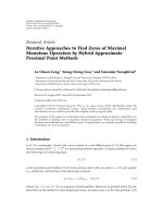
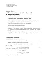
investigate the dependence of the performance on the signal length. The observed signals were simulated by convolving the source signals with impulse responses measured in
a room. The room layout is illustrated in Figure 3. The order of the impulse responses, K, was 8000. The reverberation
time was around 0.5 seconds. The signals were all sampled at
8 kHz and quantized with 16-bit resolution.
The parameter settings are listed in Table 2. The initial
estimates of the tap weights were set as
gm (k) = 0,

1 ≤ ∀m ≤ M, 1 ≤ ∀k ≤ L

while {gm (0)}1≤m≤M are fixed as (18).

(39)

Offline experiments were conducted to evaluate the fundamental performance. For each speaker and signal length,
the inverse filter was estimated by using the corresponding
observed signal. The estimated inverse filter was applied to
the observed signal to calculate the accuracy of the estimate.
Finally, for each signal length, we averaged the accuracies

over all the speakers to obtain plots such as those in Figure 4.
In Figure 4, the horizontal axis represents the signal length,
and the vertical axis represents the averaged accuracy, whose
measures are explained below.
Since the proposed algorithm estimates the inverse filters of the room acoustic system and the speech production
system, we accordingly evaluated the dereverberation performance by using two measures. One was the rapid speech
transmission index (RASTI2 ) [21], which is the most common measure for quantifying speech intelligibility from the
viewpoint of room acoustics. We used RASTI as a measure
for evaluating the accuracy of the estimated inverse filter
of the room acoustic system. According to [21], RASTI is
defined based on the modulation transfer function (MTF),
which quantifies the flattening of power fluctuations by reverberation. A RASTI score closer to one indicates higher
speech intelligibility. The other is the spectral distortion (SD)
[22] between the speech production system 1/(1 − B(z, n))
and its estimate 1/(1 − A(z, n + β)). Since the characteristics
of the speech production system can be regarded as those of
2

We used RASTI instead of the speech transmission index (STI) [21],
which is the precise version of RASTI, because calculating an STI score
requires a sampling frequency of 16 kHz or greater.


8

EURASIP Journal on Advances in Signal Processing
5.5

0.85

5
SD (dB)

RASTI score

0.9

0.8

4.5

0.75
0

2

4
6
Signal length (s)

8

4

10

0

Proposed
LS

2

4
6
Signal length (s)

8

10

Proposed
LS

Figure 4: RASTI as a function of observed signal length.

Figure 5: SD as a function of observed signal length.

0
Energy (dB)

the clean speech signal, the SD represents the extraction error of the speech characteristics. We used the SD as a measure
for assessing the accuracy of the estimated inverse filter of the
speech production sytem. The reference 1/(1 − B(z, n)) was
calculated by applying LP to the clean speech signal s(n) segmented in the same way as the recovered signal y(n).
To show the effectiveness of incorporating the nonstationarity of the innovations process (see the remark in the
last paragraph of Section 4.1), we compared the performance
of the proposed algorithm with that of an algorithm based
on the least squares (LS) criterion. The LS-based algorithm
solves

15 dB

−20
−40
−60

0

0.1

0.2

0.3

0.4

0.5

0.6

Time (s)
After
Before

Figure 6: Energy decay curves of impulse responses before and after
dereverberation.

N

d(n)2

minimize

{ai (k)},{gm (k)}

n=1

(40)

subject to 1 − Ai (z) being minimum phase.
Such an algorithm can be easily obtained by replacing the
algorithm solving (33) by the multichannel LP [16, 23].
Figure 4 shows the RASTI score averaged over the 10
speakers’ results as a function of the length of the observed
signal. Figure 5 shows the SD averaged over the results for all
time frames and speakers. There was little difference between
the results of the proposed algorithm and those of the LSbased algorithm when the length of the observed signal was
above 10 seconds. Hence, we plot the results for observed signals duration up to 10 seconds in Figures 4 and 5 to highlight
the difference between the two algorithms. We can see that
the proposed algorithm outperformed the algorithm based
on the LS criterion especially when the observed signals were
short.
We found that, among the 10 speakers, the dereverberation performance for the male speakers was a bit better than
that for the female speakers. This is probably because assumption (1) fits better for male speakers because the pitches

of male speeches are generally lower than those of female
speeches.
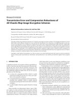
In Figure 6, we show examples of the energy decay curves
of impulse responses before and after the dereverberation obtained by using an observed signal of five seconds. A clear reduction in reflection energy can be seen; there was a 15 dB

reduction in the reverberant energy 50 milliseconds after the
arrival of the direct sound.
From the above results, we conclude that the proposed
algorithm can estimate the inverse filter of the room acoustic
system with a relatively short 3–5 second observed signal.
5.

ALGORITHM USING HIGHER-ORDER
STATISTICS

In this section, we derive an algorithm that estimates
{a(k, n)}1≤n≤N, 1≤k≤P and {gm (k)}1≤m≤M, 0≤k≤L so that the
outputs {d(n)}1≤n≤N become statistically independent of
each other. Statistical independence is a stronger requirement than the uncorrelatedness exploited by the algorithm
described in the preceding section since the independence of


Takuya Yoshioka et al.

9

random variables is characterized by both their SOS and their
HOS. Therefore, an algorithm based on the independence of
{d(n)} is expected to realize a highly accurate inverse filter
estimation because it fully uses the characteristics of the innovations process specified by assumption (1).
Before presenting the algorithm, we formulate a theorem
about the uniqueness of the estimates, {d(n)}, of the innovations {e(n)}. In this section, we also assume that
(i) the innovations {e(n)} have non-Gaussian distributions,
(ii) the innovations {e(n)} satisfy the Lindeberg condition
[24].

Under these assumptions, we have the following theorem.
Theorem 3. Suppose that variables {d(n)} are not deterministic. If {d(n)} are statistically independent with non-Gaussian
distributions, then d(n) is equalized with e(n) except for a possible scaling and delay.
Proof. The proof is deferred to Appendix E.
By using Theorems 1 and 3, it is clear that the inverse
filters of the room acoustic system and the speech production
system are uniquely identifiable.
In practice, the doubly-infinite inverse filter G(z) in (4) is
approximated by the L-tap FIR filter as
L

g(k)T x(t − k).

y(n) =

(41)

k=0

Unlike the SOS-based algorithm, we need not constrain the
first tap weights as (18). Thus, we estimate {gm (k)} with k ≥
0 in this section.
5.1. Loss function
Let us represent the mutual information of random variables
ξ1 , . . . , ξn by I(ξ1 , . . . , ξn ). By using the mutual information as
a measure of the interdependence of the random variables,
we minimize the loss function defined as I(d(1), . . . , d(N))
with respect to {a(k, n)} and {gm (k)} under the constraint
that instantaneous systems {1 − A(z, n)} are minimum phase
in a similar way to (19). The loss function can be rewritten as

(see Appendix F)

By comparing (43) with (19), it is found that (43) exploits the
negentropies of {d(n)} in addition to the correlatedness between {d(n)} as a criterion. Therefore, we try not only to uncorrelate outputs {d(n)} but also to make the distributions
of {d(n)} as far from the Gaussian as possible.
5.2.

Algorithm

As regards time variant filter 1 − A(z, n), we again use approximation (29). Then, we solve
N

minimize

{ai (k)}, {gm (k)}

J d(n) + K d(1), . . . , d(N)

−
n=1

subject to 1 − Ai (z) being minimum phase
(44)
instead of (43).
Problem (44) is solved by the alternating variables
method in a similar way to the algorithm in Section 4.
Namely, we repeat the minimization of the loss function with
respect to {ai (k)} for fixed {gm (k)} and minimization with
respect to {gm (k)} for fixed {ai (k)}. However, since the loss
function of (44) is very complicated, we derive a suboptimal

algorithm by introducing the following assumptions found
in our preliminary experiment.
(i) Given {gm (k)}, or equivalently, given y(n), the set of
parameters {ai (k)} that minimizes K(d(1), . . . , d(N))
also reduces the loss function of (44).
(ii) Given {ai (k)}, the set of parameters {gm (k)} that minimizes (− N=1 J(d(n))) also reduces the loss function
n
of (44).
With assumption (i), we again estimate {ai (k)}1≤k≤P by
applying LP to segment { y(n)}Ni ≤n≤Ni +W −1 , which is the output of G(z), for each i. It should be remembered that we can
obtain minimum-phase estimates of {1 − Ai (z)} by using LP.
Next, we estimate {gm (k)} for fixed {ai (k)} by maximizing N=1 J(d(n)) based on assumption (ii). By using the
n
Gram-Charlier expansion and retaining dominant terms, we
can approximate the negentropy J(ξ) of random variable ξ
as [26]
J(ξ)

κ3 (ξ)2
κ (ξ)2
+ 4
,
12υ(ξ)3 48υ(ξ)4

(45)

N

J d(n) + K d(1), . . . , d(N) ,

I d(1), . . . , d(N) = −
n=1

(42)
where J(ξ) denotes the negentropy [25] of random variable ξ. The computational formula of the negentropy is given
later. The negentropy represents the nongaussianity of a random variable. From (42), what we try to solve is formulated
as

where κi (ξ) represents the ith order cumulant of ξ. Generally,
the innovations of a speech signal have supergaussian distributions whose third-order cumulants are negligible compared with its fourth-order cumulants. Therefore, we finally
reach the following problem in the estimation of {gm (k)}:
N

maximize

{gm (k)}1≤m≤M, 0≤k≤L

M

N

minimize

{a(k,n)}, {gm (k)}

J d(n) +K d(1), . . . , d(N)

−

κ4 d(n)

2
υ d(n)
n=1
L

{ai (k)}={ai (k)}

(46)

2

gm (k) = 1.

subject to
m=1 k=0

n=1

subject to 1 − A(z, n) being minimum phase.
(43)

We again note that the range in k is from 0 to L unlike (33).
The constraint of (46) is intended to determine the constant


10

EURASIP Journal on Advances in Signal Processing
5.5

1

5

0.95

SD (dB)

RASTI score

4.5
0.9

4

0.85
3.5
0.8

0.75

3
2.5
0

10

20

30

40
Signal length (s)

50

60

0

scale α arbitrarily. We use the gradient method to realize this
maximization. By taking the derivative of the loss function of
(46), we have the following algorithm:

60

0.95

4

− d(n)4

d(n)2

2

(47)

RASTI score

4

d(n)2

× d(n)3 vm,i (n − k)

gm (k) =

50

1

gm (k) = gm (k)

i=1

30
40
Signal length (s)

Figure 8: SD as a function of observed signal length.

Figure 7: RASTI as a function of observed signal length.

T

20

HOS
SOS

HOS

SOS

+δ

10

0.9

0.85

d(n)2 d(n)vm,i (n − k) ,

gm (k)
M
L
2,
m=1 k=0 gm (k)

where the averages are calculated for indices Ni to Ni +W − 1.
Here, we have again used the assumption that d(n) is stationary within a single frame just as we did in the derivation of
(36).
Remark 3. While we can easily estimate {ai (k)} and {gm (k)}
with assumptions (i) and (ii), the convergence of the algorithm is not guaranteed because the assumptions may
not always be true. We examine this issue experimentally.
It is hoped that future work will reveal the theoretical background to the assumptions.
5.3. Experimental results
We compared the dereverberation performance of the HOSbased algorithm proposed in this section with that of the
SOS-based algorithm described in the previous section. We
used the same experimental setup as that in the previous section except for the iteration parameters R1 and R2 , which we
set at 10 and 20, respectively.

Figure 7 shows the RASTI score averaged over the 10
speakers’ results as a function of the length of the observed

0.8

0.75

0

2
4
6
8
Number of alternations of ai (k) and gm (k)
3 seconds
4 seconds
5 seconds

10

10 seconds
20 seconds
1 minute

Figure 9: RASTI as a function of iteration number.

signal. As expected, we can see that the HOS-based algorithm
outperformed the SOS-based algorithm when the observed
signal was relatively long. In particular, when an observed
signal of longer than 20 seconds was available, the RASTI

score was nearly equal to one. Figure 8 shows the average
SD. Again, we can confirm the great superiority of the HOSbased algorithm to the SOS-based algorithm in terms of
asymptotic performance.
In Figure 9, we plot the average RASTI score as a function of the number of alternations of estimation parameters {ai (k)} and {gm (k)}. We can clearly see the convergence


Takuya Yoshioka et al.

11

1
×10−2

0.95
Normalized number
of appearance

5

RASTI score

0.9
0.85
0.8

10

20

30

SNR (dB)

SOS, 5 seconds
SOS, 20 seconds

40

Inf.

HOS, 5 seconds
HOS, 20 seconds

Figure 10: RASTI obtained in the presence of noise.

1

DISCUSSION

6.1. Effect of additive noise
Thus far, we have considered a system without any additive
noise. In this section, we experimentally examine the effect
of additive noise on the performance of the proposed algorithms3 .
We tested a case where the observed signal was contaminated by additive white Gaussian noise with signal to
noise ratios (SNR) of 40, 30, 20, and 10 dB. Since the proposed methods do not involve noise reduction, we measured the performance as a RASTI score calculated by using the impulse response of equalized room acoustic system
G(z)T H(z).
In Figure 10, we plot the average RASTI scores as a function of the SNR for observed signals of five and twenty seconds. The SOS-based algorithm was relatively robust against
additive noise. Although the performance of the HOS-based
algorithm was degraded more severely than that of the SOSbased algorithm, the former still exhibited excellent performance in the presence of noise with an SNR of 30 dB or
greater when the observed signal was 20 seconds long.
Thus, it is a promising way to combine the proposed

algorithms with traditional noise reduction methods such
as spectral subtraction [28] in a noisy environment with a

We also conducted an experiment by using real recordings where the
room acoustic system might fluctuate and where there was slight background noise. Good dereverberation performance was achieved in this
experiment. The result is reported in [27].

0

ry p −0.5
ar t

−1

−1

−0.5

0

0.5

1

part
Real

Figure 11: Histogram showing the number of poles of the speech
production system in each small region in the complex plane.

severe SNR. An investigation of such a combination is however beyond the scope of this paper.
6.2.

of the RASTI score. The RASTI score converges particularly
rapidly when the observed signal length is sufficiently large.

3

2

0.5
Im
ag i
na

0.7

6.

3

0
1

0.75

0.65

4

Validity of assumption (2)

Assumption (2) is one of the essential assumptions that form
the basis of the proposed algorithms. Here we investigate its
validity.
Figure 11 is an example histogram showing the number
of poles of the speech production system included in a clean
speech signal of five seconds in each small region in the complex plane. The number of poles in each region is normalized
by the total frame number. Due to this normalization, regions with a value of one correspond to time invariant poles.
In Figure 11, we can see no such regions, which indicates that
there is no time invariant pole. This result supports assumption (2).
7.

CONCLUSION

We have described the problem of speech dereverberation.
The contribution of this paper is summarized as follows.
(i) We proposed the joint estimation of the time invariant
and time variant subfilters of the inverse filter of an
overall acoustic system. It was shown that these subfilters correspond to the inverse filters of a room acoustic
system and a speech production system, respectively.
(ii) We developed two distinct algorithms; one uses a criterion based on the SOS of the output while the other is
based on the HOS. The SOS-based algorithm improves
RASTI by 0.1 even when the observed signals are at
most 5-second long. By contrast, the HOS-based algorithm estimates the inverse filter with a RASTI score of
nearly one, as long as observed signals of longer than
20 seconds are available.
The main purpose of this paper is to elucidate the theoretical background of the joint estimation based speech
dereverberation and the corresponding algorithms and to
evaluate their fundamental performance. Thus, we have not

12

EURASIP Journal on Advances in Signal Processing

investigated practical issues such as computational costs and
adaptation to time varying environments. A simple way to
cope with these issues would be to employ stochastic gradient learning. An exaustive subjective listening test should also
be conducted. Investigating these issues in depth is a subject
for future study.
APPENDICES
A.

Relation Σ(d) = E{ddT } = AE{yyT }AT = AΣ(y)AT
leads to
log det Σ(d) = log det Σ(y) + 2 log | det A|.

Because the determinant of an upper triangular matrix is
the product of its diagonal components, we have det A = 1.
Hence, we obtain
log det Σ(d) = log det Σ(y) .

PROOF OF THEOREM 1
1 − A(z, n) G(z)T H(z) s(n).

M

(A.1)

y=

Substituting (15) into (A.1) yields
αe(n − β) =

(A.2)

On the other hand, from (9), we have

This equation is equivalent to
e(n − β) = 1 − B(z, n − β)z−β s(n).

(A.4)

Relations (A.2) and (A.4) give
1 − A(z, n) G(z)T H(z)

where xm , Gm , and Hm are written as
⎡

⎢
⎢
⎢
⎢
⎢
Gm = ⎢
⎢
⎢
⎢
⎣

(A.5)

⎡

Since both 1 − A(z, n) and 1 − B(z, n) have no time invariant
zero according to (16) and (11), we have

⎢
⎢
⎢
⎢
⎢
Hm = ⎢
⎢
⎢
⎢
⎣

1 ≤ ∀n ≤ N.

G(z)T H(z) = αz−β .

(A.6)

DERIVATION OF (26)

In this appendix, we show that log | det Σ(d)| is invariant with respect to {a(k, n)}1≤n≤N, 1≤k≤P and
{gm (k)}1≤m≤M, 1≤k≤L . We here assume that s(n) = 0
when n ≤ 0. Hence, relation (B.10), which we derive here,

may be an approximation.
Output vector d, defined by (25), is represented by using
y = [y(N), . . . , y(1)]T as
d = Ay,

⎢
⎢
⎢
⎢
⎢
⎢
⎢
⎢
⎢
⎢
⎢
⎢
⎢
⎢
⎢
⎢
⎢
⎢
⎢
⎢
⎢
⎢
⎢
⎢
⎢

⎣

1

(B.6)

⎤

hm (0) · · · hm (K)
O
⎥
⎥
..
..
⎥
.
.
⎥
⎥
hm (0) · · · hm (K)⎥ .
⎥
. ⎥
..
. ⎥
.
. ⎦
O
hm (0)

Hence, in a similar way to (B.3), we obtain

M

log det Σ(y) = log det Σ(s) + 2 log det

Gm Hm
m=1

M

= 2 log det

Gm Hm

+ constant.

m=1

(B.7)
Since M=1 Gm Hm is also an upper triangular matrix with
m
diagonal elements of M=1 hm (0)gm (0), we have
m

A=
···

⎤

gm (0) · · · gm (L)
O

⎥
⎥
..
..
⎥
.
.
⎥
⎥
gm (0) · · · gm (L)⎥ ,
⎥
. ⎥
..
. ⎥
.
. ⎦
O
gm (0)

(B.1)

where A is defined as (B.2):
1 −a(1, N)

(B.5)

T

(A.3)

⎡

Gm Hm s,
m=1

xm = xm (N), . . . , xm (1) ,

e(n) = 1 − B(z, n) s(n) = 1 − B(z, n)z−β s(n + β).

B.

M

Gm xm =
m=1

1 − A(z, n) G(z)T H(z) s(n).

= 1 − B(z, n − β) αz−β ,

(B.4)

y is related to s = [s(N), . . . , s(1)]T as

By using (2), (5), and (13), we obtain
d(n) =

(B.3)

⎤

· · · −a(P, N)

⎥
⎥
⎥
−a(1, N −1) · · · · · ·
−a(P, N −1)
⎥
⎥
⎥
..
..
⎥
⎥
.
.
⎥
⎥
···
· · · −a(P, P+1) ⎥
1 −a(1, P+1)
⎥
⎥
⎥.
1
−a(1, P) · · · −a(P−1, P)⎥
⎥
⎥
⎥

.
⎥
..
..
.
⎥
.
.
.
⎥
⎥
⎥
1 −a(1, 2) ⎥
⎥
⎦

1
(B.2)

M

M

Gm Hm

log det

= N log

m=1

hm (0)gm (0) .
m=1

(B.8)
Substituting (18) into (B.8) yields
M

Gm Hm

log det

= N log h1 (0) = constant.

m=1

(B.9)
By using (B.3), (B.7), and (B.9), we can derive
log det Σ(d) = constant.

(B.10)


Takuya Yoshioka et al.

13

C. PROOF OF THEOREM 2

D.

By (4) and (12), d(n) is written by using {s(n − k)}0≤k≤K+L+P
as

DERIVATION OF (36)

By using the assumption that d(n) is stationary within a single frame and replacing the variance υ(d(n)) by its sample
estimate, the loss function of (33), N=1 log υ(d(n)), is estin
mated by

d(n) = h1 (0)s(n) + Lc s(n − k); 1 ≤ k ≤ K + L + P ,
(C.1)

T

W log d(n)2
i=1

where Lc {·} stands for the linear combination. By substituting (8) into (C.1), d(n) is rewritten as

Ni +W −1
n=Ni

log d(n)2
i=1

Ni +W −1
.
n=Ni

(D.1)

The derivative of the right-hand side of (D.1) with respect to
gm (k) is
T

d(n) = h1 (0)e(n) + u n; G(z), A(z, n) ,

T

∝

∂
log d(n)2
∂gm (k) i=1

(C.2)

T

∂d(n)
d(n)
∂gm (k)

2

=

d(n)2

i=1

where u(n) is of the form

Ni +W −1
n=Ni

Ni +W −1
n=Ni

(D.2)

Ni +W −1
n=Ni

.

The derivative of d(n) belonging to the ith frame is
u(n) = Lc s(n − k); 1 ≤ k ≤ K + L + P .

P
∂y(n − l)
∂y(n)
∂d(n)
=
−
ai (l)
∂gm (k) ∂gm (k) l=1
∂gm (k)

(C.3)

P

Because s(n) is of the form

= xm (n − k) −

ai (l)xm (n − l − k)

(D.3)

l=1

s(n) = Lc e(n), s(n − k); 1 ≤ k ≤ P

= vm,i (n − k).

(C.4)

From (D.2) and (D.3), we have the update equation of (36).
as in (8), s(n) has no components of {e(n+k)}k≥1 . Therefore,
e(n) and u(n) are statistically independent. Then, we have

υ d(n) = h1 (0)2 υ e(n) + υ u(n) ≤ h1 (0)2 υ e(n)
(C.5)

with equality if and only if

υ u(n) = 0.

1 ≤ ∀n ≤ N.

PROOF OF THEOREM 3

Let { f (k, n)}−∞≤k≤∞ be the impulse response of the global
system (1 − A(z, n))G(z)T H(z)/(1 − B(z, n)) at time n. Since
d(n) has a non-Gaussian distribution, sequence { f (k, n)} has
finite nonzero components according to the central limit theorem [24]. Because d(n) is not deterministic, { f (k, n)} has at
least one nonzero component. Let the first nonzero component of { f (k, n)} be f (βn , n). Since the time variant part of
the global system (1 − A(z, n))G(z)T H(z)/(1 − B(z, n)) has
the first tap of weight one, we have

(C.6)

Because the logarithmic function is increasing monotonically, N=1 log υ(d(n)) reaches a minimum if and only if
n
υ u(n) = 0,

E.

βm = β n ,

f βm , m = f βn , n ,

∀m, ∀n.

(E.1)

So we can represent the index and value of the first nonzero

component as β and α, respectively. Because variables {d(n)}
are independent, we obtain the following relation by using
Darmois’ theorem [25]:
f (k, n) f (k − m, n − m) = 0,

(C.7)

∀n, ∀k, ∀m = 0.

(E.2)

If
According to (C.2), condition (C.7) is satisfied if and only if
d(n) is equalized with e(n) as

k = β + m,

(E.3)

we have
d(n) = h1 (0)e(n).

(C.8)

f (k − m, n − m) = f (β, n − m) = α = 0.

(E.4)


14

EURASIP Journal on Advances in Signal Processing

Therefore, if m = 0, we obtain by using (E.2)
f (k, n) = f (β + m, n) = 0.

(E.5)

Furthermore, since y is related to s by an N × N regular linear transformation according to (B.5), and the negentropy is
conserved by such linear transformation, we obtain

Thus, { f (k, n)} has only one nonzero component f (β, n) =
α. Since d(n) is represented as
1 − A(z, n) G(z)T H(z)
e(n),
1 − B(z, n)

d(n) =

(E.6)

d(n) is equalized with e(n) up to constant scale α and delay
β.
F.

DERIVATION OF (40)

Mutual information I(d(1), . . . , d(N)) is defined as
N

I d(1), . . . , d(N) =

H d(n) − H (d),

(F.1)

n=1

where H (ξ) represents the differential entropy of (multivariate) random variable ξ. From (B.1), we have
H (d) = H (y) + log | det A|.

(F.2)

Because of (B.3), we also have
1
log det Σ(d) − log det Σ(y) .
2
Substituting (F.2) and (F.3) into (F.1) gives
log | det A| =

(F.3)

I d(1), . . . , d(N)
N

H d(n) −

=
n=1

+

1
log det Σ(y) − H (y)
2
N

=−
n=1

+

1
log det Σ(d)
2

1
2

1
log υ d(n) − H d(n)
2

(F.4)

N

log υ d(n) − log det Σ(d)
n=1

1
log det Σ(y) − H (y).
2
Now, the negentropy of n-dimensional random variable ξ is
defined as
+

J(ξ) = H ξ gauss − H (ξ)
=

1
log det Σ ξ gauss
2

n
+ (1 + log 2π) − H (ξ),
2
(F.5)

where ξ gauss is a Gaussian random variable with the same covariance matrix as that of ξ. By using (20) and (F.5), (F.4) is
rewritten as
I d(1), . . . , d(N)
N

J d(n) + J(y) + K d(1), . . . , d(N) .

=−
n=1

(F.6)

J(y) = constant.

(F.7)

From (F.6) and (F.7), we finally reach (42).
REFERENCES
[1] L. R. Rabiner and R. W. Schafer, Digital Processing of Speech
Signals, Prentice-Hall, Upper Saddle River, NJ, USA, 1983.
[2] M. I. Gurelli and C. L. Nikias, “EVAM: an eigenvector-based
algorithm for multichannel blind deconvolution of input colored signals,” IEEE Transactions on Signal Processing, vol. 43,
no. 1, pp. 134–149, 1995.
[3] K. Furuya and Y. Kaneda, “Two-channel blind deconvolution
of nonminimum phase FIR systems,” IEICE Transactions on
Fundamentals of Electronics, Communications and Computer
Sciences, vol. E80-A, no. 5, pp. 804–808, 1997.
[4] S. Gannot and M. Moonen, “Subspace methods for multimicrophone speech dereverberation,” EURASIP Journal on Applied Signal Processing, vol. 2003, no. 11, pp. 1074–1090, 2003.
[5] T. Hikichi, M. Delcroix, and M. Miyoshi, “Blind dereverberation based on estimates of signal transmission channels without precise information on channel order,” in IEEE International Conference on Acoustics, Speech, and Signal Processing
(ICASSP ’05), vol. 1, pp. 1069–1072, Philadelphia, Pa, USA,
March 2005.
[6] M. Delcroix, T. Hikichi, and M. Miyoshi, “Precise dereverberation using multichannel linear prediction,” IEEE Transactions
Audio, Speech and Language Processing, vol. 15, no. 2, pp. 430–
440, 2007.
[7] B. Yegnanarayana and P. S. Murthy, “Enhancement of reverberant speech using LP residual signal,” IEEE Transactions on
Speech and Audio Processing, vol. 8, no. 3, pp. 267–281, 2000.
[8] B. W. Gillespie, H. S. Malvar, and D. A. F. Florˆ ncio, “Speech
e
dereverberation via maximum-kurtosis subband adaptive filtering,” in IEEE Interntional Conference on Acoustics, Speech,
and Signal Processing (ICASSP ’01), vol. 6, pp. 3701–3704, Salt
Lake, Utah, USA, May 2001.

[9] B. W. Gillespie and L. E. Atlas, “Strategies for improving audible quality and speech recognition accuracy of reverberant
speech,” in IEEE International Conference on Accoustics, Speech,
and Signal Processing (ICASSP ’03), vol. 1, pp. 676–679, Hong
Kong, April 2003.
[10] N. D. Gaubitch, P. A. Naylor, and D. B. Ward, “On the use
of linear prediction for dereverberation of speech,” in Proceedings of International Workshop on Acoustic Echo and Noise
Control (IWAENC ’03), pp. 99–102, Kyotp, Japan, September
2003.
[11] T. Nakatani, K. Kinoshita, and M. Miyoshi, “Harmonicitybased blind dereverberation for single-channel speech signals,” IEEE Transactions, Audio, Speech and Language Processing, vol. 15, no. 1, pp. 80–95, 2007.
[12] K. Kinoshita, T. Nakatani, and M. Miyoshi, “Efficient blind
dereverberation framework for automatic speech recognition,” in Proceedings of the 9th European Conference on Speech
Communication and Technology, pp. 3145–3148, Lisbon, Portugal, September 2005.


Takuya Yoshioka et al.
[13] P. S. Spencer and P. J. W. Rayner, “Separation of stationary and
time-varying systems and its application to the restoration of
gramophone recordings,” in IEEE International Symposium on
Circuits and Systems (ISCAS ’89), vol. 1, pp. 292–295, Portland,
Ore, USA, May 1989.
[14] J. R. Hopgood and P. J. W. Rayner, “Blind single channel
deconvolution using nonstationary signal processing,” IEEE
Transactions on Speech and Audio Processing, vol. 11, no. 5, pp.
476–488, 2003.
[15] O. Shalvi and E. Weinstein, “New criteria for blind deconvolution of nonminimum phase systems(channels),” IEEE Transactions on Information Theory, vol. 36, no. 2, pp. 312–321,
1990.
[16] K. Abed-Meraim, E. Moulines, and P. Loubaton, “Prediction error method for second-order blind identification,” IEEE
Transactions on Signal Processing, vol. 45, no. 3, pp. 694–705,
1997.
[17] B. Theobald, S. Cox, G. Cawley, and B. Milner, “Fast method

of channel equalisation for speech signals and its implementation on a DSP,” Electronics Letters, vol. 35, no. 16, pp. 1309–
1311, 1999.
[18] D.-T. Pham and J.-F. Cardoso, “Blind separation of instantaneous mixtures of nonstationary sources,” IEEE Transactions
on Signal Processing, vol. 49, no. 9, pp. 1837–1848, 2001.
[19] K. Matsuoka, M. Ohya, and M. Kawamoto, “A neural net for
blind separation of nonstationary signals,” Neural Networks,
vol. 8, no. 3, pp. 411–419, 1995.
[20] Acoustical Society of Japan, “ASJ Continuous Speech Corpus,”
/>[21] H. Kuttruff, Room Acoustics, Elsevier Applied Science, London,
UK, 1991.
[22] W. B. Kleijn and K. K. Paliwal, Eds., Speech Coding and Synthesis, Elsevier Science, Amsterdam, The Netherlands, 1995.
[23] A. Gorokhov and P. Loubaton, “Blind identification of
MIMO-FIR systems: a generalized linear prediction approach,” Signal Processing, vol. 73, no. 1-2, pp. 105–124, 1999.
[24] J. Jacod and A. N. Shiryaev, Limit Theorems for Stochastic Processes, Springer, New York, NY, USA, 1987.
[25] P. Comon, “Independent component analysis, a new concept?” Signal Processing, vol. 36, no. 3, pp. 287314, 1994.
[26] A. Hyvă rinen, J. Karhumen, and E. Oja, Independent Compoa
nent Analysis, John Wiley & Sons, New York, NY, USA, 2001.
[27] T. Yoshioka, T. Hikichi, M. Miyoshi, and H. G. Okuno, “Robust decomposition of inverse filter of channel and prediction error filter of speech signal for dereverberation,” in Proceedings of the 14th European Signal Processing Conference
(EUSIPCO ’06), Florence, Italy, 2006.
[28] S. F. Boll, “Suppression of acoustic noise in speech using
spectral subtraction,” IEEE Trans Acoust Speech Signal Process,
vol. 27, no. 2, pp. 113–120, 1979.

Takuya Yoshioka received the M.S. of Informatics degree from Kyoto University, Kyoto,
Japan, in 2006. He is currently with the Signal Processing Group of NTT Communication Science Laboratories. His research interests are in speech and audio signal processing and statistical learning.

15
Takafumi Hikichi was born in Nagoya, in
1970. He received his B.S. and M.S. of
electrical engineering degrees from Nagoya

University in 1993 and 1995, respectively.
In 1995, he joined the Basic Research Laboratories of NTT. He is currently working
at the Signal Processing Research Group of
the Communication Science Laboratories,
NTT. He is a Visiting Associate Professor
of the Graduate School of Information Science, Nagoya University. His research interests include physical
modeling of musical instruments, room acoustic modeling, and
signal processing for speech enhancement and dereverberation. He
received the 2000 Kiyoshi-Awaya Incentive Awards, and the 2006
Satoh Paper Awards from the ASJ. He is a Member of IEEE, ASA,
ASJ, and IEICE.
Masato Miyoshi received his M.E. degree
from Doshisha University in Kyoto in 1983.
Since joining NTT as a Researcher that year,
he has been studying signal processing theory and its application to acoustic technologies. Currently, he is the leader of the Signal
Processing Group, the Media Information
Laboratory, NTT Communication Science
Labs. He is also a Visiting Associate Professor of the Graduate School of Information
Science and Technology, Hokkaido University. He was honored to
receive the 1988 IEEE senior awards, the 1989 ASJ Kiyoshi-Awaya
incentive awards, the 1990 and 2006 ASJ Sato Paper awards, and the
2005 IEICE Paper awards, respectively. He also received his Ph.D.
degree from Doshisha University in 1991. He is a Member of IEICE, ASJ, AES, and a Senior Member of IEEE.