Báo cáo hóa học: " Research Article Human Hand Recognition Using IPCA-ICA Algorithm" doc

Hindawi Publishing Corporation
EURASIP Journal on Advances in Signal Processing
Volume 2007, Article ID 91467, 7 pages
doi:10.1155/2007/91467
Research Article
Human Hand Recognition Using IPCA-IC A Algorithm
Issam Dagher, William Kobersy, and Wassim Abi Nader
Department of Computer Engineering, University of Balamand, Elkoura, Lebanon
Received 3 July 2006; Revised 21 November 2006; Accepted 2 February 2007
Recommended by Satya Dharanipragada
A human hand recognition system is introduced. First, a simple preprocessing technique which extracts the palm, the four fingers,
and the thumb is introduced. Second, the eigenpalm, the eigenfingers, and the eigenthumb features are obtained using a fast incre-
mental principal non-Gaussian directions analysis algorithm, called IPCA-ICA. This algorithm is based on merging sequentially
the runs of two algorithms: the principal component analysis (PCA) and the independent component analysis (ICA) algorithms.
It computes the principal components of a sequence of image vectors incrementally without estimating the covariance matrix (so
covariance-free) and at the same time transforming these principal components to the independent directions that maximize the
non-Gaussianity of the source. Third, a classification step in which each feature representation obtained in the previous phase is
fed into a simple nearest neighbor classifier. The system was tested on a database of 20 people (100 hand images) and it is compared
to other algorithms.
Copyright © 2007 Issam Dagher et al. This is an open access article distributed under the Creative Commons Attribution License,
which permits unrestricted use, distribution, and reproduction in any medium, provided the original work is properly cited.
1. INTRODUCTION
Biometrics is an emerging technology [1, 2] that is used to
identify people by their physical and/or behavioral character-
istics and, so, inherently requires that the person to be iden-
tified is physically present at the point of identification. The
physical characteristics of an individual that can be used in
biometric identification/verification systems are fingerprint
[3, 4], hand geometry [5, 6], palm print [7–9], face [4, 10],
iris [11, 12], retina [13], and the ear [14].
The behavioral characteristics are signature [12], lip

movement [15], speech [16], keystroke dynamics [1, 2], ges-
ture [1, 2], and the gait [1, 2].
A single physical or behavioral characteristic of an in-
dividual can sometimes be insufficient for identification.
For this reason, multimodal biometric systems—that is,
systems that integrate two or more different biometrics
characteristics—are being developed to provide an accept-
able performance, and increase the reliability of decisions.
The human hand contains a wide variety of features, for ex-
ample, shape, texture, and principal palm lines—that can be
used by biometric systems. Features extracted by projecting
palm images into the subspace obtained by the PCA trans-
form are called eigenpalm features, whereas those extracted
by projecting images of fingers and thumb are called eigen-
finger and eigenthumb features. This paper merges sequen-
tially two techniques based on principal component analysis
and independent component analysis.
The first technique is called incremental principal com-
ponent analysis (IPCA) which is an incremental version of
the popular unsupervised principal component technique.
The traditional PCA [17] algorithm computes eigenvectors
and eigenvalues for a sample covariance matrix derived from
a well-known given image data matrix, by solving an eigen-
value system problem. Also, this algorithm requires that
the image data matrix be available before solving the prob-
lem (batch method). The incremental principal component
method updates the eigenvectors each time a new image is
introduced.
The second technique is called independent component
analysis (ICA) [18]. It is used to estimate the independent

characterization of human hand vectors (palms, fingers, or
thumbs). It is known that there is a correlation or depen-
dency between different human hand vectors. Finding the
independent basic vectors that form those correlated ones
is a very important task. The set of human hand vectors is
represented as a data matrix X where each row corresponds
to a different human hand. The correlation between rows
of matrix X can be represented as the rows of a mixing
matrix A. The independent basic vectors are represented as
rows of source matrix S. The ICA algorithm extr acts these
2 EURASIP Journal on Advances in Signal Processing
independent vectors from a set of dependent ones using
X
= A · S. (1)
When the dimension of the image is high, both the com-
putation and storage complexity grow dramatically. Thus,
the idea of using a real time process becomes very efficient
in order to compute the principal independent components
for observations arriving sequentially. Each eigenvector
or principal component will be updated, using FastICA
algorithm, to a non-Gaussian component. In (1), if the
source matrix S contains Gaussian uncorrelated elements
then the resulting elements in the mixed matrix X will be
also Gaussian but correlated elements.
The FastICA method does not have a solution if the ran-
dom variables to estimate are Gaussian random variables.
This is due to the fact that the joint distribution of the ele-
ments of X will be completely symmetric and does not give
any special information about the columns of A. In this pa-
per, S is always a non-Gaussian vector. It should be noted that

the centra l limit theorem states that the sum of several inde-
pendent random variables, such as those in S, tends towards
a Gaussian distribution. So x
i
= a
1
s
1
+ a
2
s
2
is more Gaussian
than either s
1
or s
2
. The central limit theorem implies that if
we can find a combination of the measured signals in X with
minimal Gaussian properties, then that signal will be one of
the independent signals. Once W is determined it is a simple
matter to invert it to find A.
Each image x, represented by an (n, m) matrix of pixels,
will be represented by a high-dimensional vector of n
×m pix-
els. These image vectors w ill be the rows of X and the result-
ing uncorrelated components will be the rows of S. There-
fore, each column of A, called w, will be a direction that max-
imizes the non-Gaussianity of the projection of the depen-
dent images x into w. The raw features that are sent to this

algorithm are the grayscale levels of every pixel in the image
without using any geometric features or wavelet-based fea-
tures.
It should be noted that the batch method no longer sat-
isfies an up coming new trend of signal processing research
in which all visual filters are incrementally derived from very
long online real-time video stream. Online development of
visual filters requires that the system perform while new sen-
sory signals flow in. When the dimension of the image is
high, both the computation and storage complexity grow
dramatically. Thus, the idea of using a real time process be-
comes very efficient in order to compute the principal in-
dependent components for observations (faces) arriving se-
quentially.
2. SYSTEM DESCRIPTION
The multimodal biometric identification system consists of
the following phases.
(i) The image-acquisition phase: a hand image is taken us-
ing a low-cost scanner; the spatial resolution of the im-
ages is 180 dots per inch (dpi) and 256 gray levels.
(ii) The preprocessing phase: three regions of interest are
localized: a palm region, four-finger region, and the
thumb region.
(iii) The processing phase: the three normalized regions
are transformed by the sequential PCA-ICA algorithm
into three spaces called eigenpalm space, eigenfinger
space, and eigenthumb space. The feature spaces are
spanned by a certain number of the largest eigenvec-
tors. The outputs of the feature-extraction modules,
for the sample x, are three feature vectors.

(iv) The recognition phase: the matching between the cor-
responding vectors and the templates from a database
is performed.
3. PREPROCESSING PHASE
Images of the right hand are scanned at 180 dpi/256 gr ay lev-
els using a low-cost scanner. The user puts his/her hand on
the scanner with the fingers spread naturally; there are no
pegs, or any other hand-position constrainers.
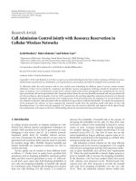
Figure 1 shows the separation the hand image of all users
into three different regions.
The regions are the thumb image (Figure 1(e)), the palm
(Figure 1(d)), and the remaining four fingers ( Figure 1(c)).
Figure 1(b) shows that the calculations of the regions is
quite simple and requires no hard or long processing time,
simply the four-fingers region is separated from the other
two by taking a horizontal line at 45 percent of the original
image. Then, the palm region is obtained by a vertical line at
70 percent of the subimage obtained before.
The method described above is applied to all users’ im-
ages since the entire scanned are acquired having 1020
× 999
pixels.
After acquiring and obtaining three regions, a geometry
normalization is also applied and the “four-fingers” region is
normalized to 454
×200 pixels, the “palm” region to 307×300
pixels, and the “thumb” region to 180
× 300 pixels.
4. DERIVATION OF THE IPCA-ICA ALGORITHM
Each time a new image is introduced, the non-Gaussian vec-

tors will be updated. They are presented by the algorithm in
a decreasing order with respect to the corresponding eigen-
value (the first non-Gaussian vector will correspond to the
largest eigenvalue). While the convergence of the first non-
Gaussian vector will be shown in Section 4.1, the conver-
gence of the other vectors will be shown in Section 4.2.
4.1. The first non-Gaussian vector
4.1.1. Algorithm definition
Suppose that the sample d-dimensional vectors, u(1); u(2);
, possibly infinite, which are the observations from a cer-
tain given image data, are received sequentially. Without loss
of generality, a fixed estimated mean image is initialized in
the beginning of the algorithm. It should be noted that a
simple way of getting the mean image is to present sequen-
tially all the images and calculate their mean. This mean
Issam Dagher et al. 3
(a)
45%
70%
(b)
(c)
(d) (e)
Figure 1: (a) original image. (b) original image with regions of in-
terest marked. (c) “four-fingers” subimage. (d) “palm” subimage.
(e) “thumb” subimage.
Image 1
Image 2
Image n
v
1

(1) v
2
(1)
v
k
(1)
v
1
(2) v
2
(2) v
k
(2)
v
1
(n) v
2
(n) v
k
(n)
···
···
···
.
.
.
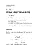
Figure 2: IPCA-PCA algorithm description.
canbesubtractedfromeachvectoru(n)inordertoob-
tain a normalization vector of approximately zero mean. Let
C

= E[u(n)u
T
(n)] be the d × d covariance matrix, which
is not known as an intermediate result. The IPCA-ICA algo-
rithm can b e described as follows.
The proposed algorithm takes the number of input im-
ages, the dimension of the images, and the number of de-
sired non-Gaussian directions as inputs and returns the im-
age data matrix, and the non-Gaussian vectors as outputs. It
works like a linear system that predicts the next state vec-
tor from an input vector and a current state vector. The
non-Gaussian components will be updated from the previ-
ous components values and from a new input image vector
by processing sequentially the IPCA and the FastICA algo-
rithms. While IPCA returns the estimated eigenvectors as a
matrix that represents subspaces of data and the correspond-
ing eigenvalues as a row vector, FastICA searches for the in-
dependent directions w where the projections of the input
data vectors will maximize the non-Gaussianity. It is based
on minimizing the approximate negentropy function [19]
given by J(x)
=

i
k
i
{E(G
i
(x)) − E(G
i

(v))}
2
using Newton’s
method. Where G(x) is a nonquadratic function of the ran-
dom variable x and E is its expected value.
The obtained independent vectors will form a basis
which describes the original data set without loss of infor-
mation. The face recognition can be done by projecting the
input test image onto this basis and comparing the resulting
coordinates with those of the training images in order to find
the nearest appropriate image.
Assume the data consists of n images and a set of k non-
Gaussian vectors are given, Figure 2 illustrates the steps of the
algorithm.
Initially, all the non-Gaussian vectors are chosen to de-
scribe an orthonor mal basis. In each step, all those vectors
4 EURASIP Journal on Advances in Signal Processing
Input
image
IPCA ICA
IPCA ICA
IPCA ICA
First estimated
non-Gaussian
vector
Second estimated
non-Gaussian
vector
Last estimated
non-Gaussian

vector
.
.
.
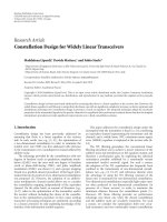
Figure 3: IPCA-ICA algorithm block diagram.
will be updated using an IPCA updating rule presented in
(7). Then each estimated non-Gaussian vector will be an in-
put for the ICA function in order to extract the correspond-
ing non-Gaussian vector from it (Figure 3).
4.1.2. Algorithm equations
By definition, an eigenvector x with a corresponding eigen-
value λ of a covariance matrix C satisfies
λ
· x = C · x. (2)
By replacing in (2) the unknown C with the sample covari-
ance matrix (1/n)

n
i=1
u(i) · u
T
(i) and using v = λ · x, the
following equation is obtained:
v(n)
=
1
n
n

i=1

u(i) · u
T
(i) · x(i), (3)
where v(n) is the nth step estimate of v after entering all the
n images.
Since λ
=v and x = v/v, x(i)issettov(i−1)/v(i −
1) (estimating x(i) according to the given previous value of
v). Equation (3) leads to the following equation:
v(n) =
1
n
n

i=1
u(i) · u
T
(i) ·
v(i − 1)


v(i − 1)


. (4)
Equation (4)canbewritteninarecursiveform:
v(n)
=
n − 1
n

v(n
− 1) +
1
n
u(n)u
T
(n)
v(n
− 1)


v(n − 1)


,(5)
where (n
− 1)/n is the weight for the last estimate and 1/n is
the weight for the new data.
To begin w ith, let v(0)
= u(1) the first direction of data
spread. The IPCA algorithm will give the first estimate of the
first principal component v(1) that corresponds to the max-
imum eigenvalue:
v(1)
= u(1)u
T
(1)
v(0)



v(0)


. (6)
Then, the vector will be the initial direction in the Fas-
tICA algorithm:
w
= v(1). (7)
The FastICA algorithms will repeat until convergence the
following rule:
w
new
= E

v(1) · G


w
T
· v(1)

−
E

G


w
T
· v(1)


·
w,
(8)
where G

(x) is the derivative of the function G

(x)(equation
(10)). It should be noted that this algorithm uses an approxi-
mation of negentropy in order to assure the non-Gaussianity
of the independent vectors. Before starting the calculation of
negentropy, a nonquadratic function G should be chosen, for
example,
G(u)
=−exp

−
u
2
2

,(9)
and its derivative:
G

(u) = u · exp

−
u

2
2

. (10)
In general, the corresponding non-Gaussian vector w,for
the estimated eigenvectors v
k
(n), will be estimated using the
following repeated rule:
w
new
= E

v
k
(n) · G


w
T
· v
k
(n)

−
E

G



w
T
· v
k
(n)

·
w.
(11)
4.2. Higher order non-Gaussian vectors
The previous discussion only estimates the first non-Gauss-
ian vector. One way to compute the other higher order vec-
tors is following what stochastic gradient ascent (SGA) does:
start with a set of orthonormalized vectors, update them us-
ing the suggested iteration step, and recover the orthogonal-
ity using Gram-Schmidt orthonormalization (GSO). For real-
time online computation, avoiding time-consuming GSO is
needed. Further, the non-Gaussian vectors should be orthog-
onal to each other in order to ensure the independency. So,
it helps to generate “observations” only in a complementary
space for the computation of the higher order eigenvectors.
For example, to compute the second order non-Gaussian
vector, first the data is subtracted from its projection on the
estimated first-order eigenvector v
1
(n), as shown in:
u
2
(n) = u
1

(n) − u
T
1
(n)
v
1
(n)


v
1
(n)


v
2
(n)


v
2
(n)


, (12)
where u
1
(n) = u(n). The obtained residual, u
2
(n), which is

in the complementary s pace of v
1
(n), serves as the input data
to the iteration step. In this way, the orthogonality is always
enforced when the convergence is reached, although not ex-
actly so at early stages. This, in effect, better uses the sample
available and avoids the time-consuming GSO.
After convergence, the non-Gaussian vector will also be
enforced to be orthogonal, since they are estimated in com-
plementary spaces. As a result, all the estimated vectors w
k
will be
Issam Dagher et al. 5
For i = 1:n
img = input image from image data matrix;
u(i)
= img;
for j
= 1:k
if j
== i, initialize the jth non-Gaussian
vector as
v
j
(i) = u(i);
else
v
j
(i) =
i − 1

i
v
j
(i − 1) +
1
i
u(i)u
T
(i)
v
j
(i − 1)


v
j
(i − 1)


; (vector update)
u(i) = u(i) − u
T
(i) ·
v
j
(i)


v
j

(i)


v
j
(i)


v
j
(i)


; (to ensure orthogonality)
end
w
= v
j
(i);
Repeat until convergence (wnew
= w)
w
new
= E

v
j
(i) · G



w
T
· v
j
(i)

−
E

G


w
T
· v
j
(i)

] · w;
(searching for the direction that
maximizes non-Gaussianity)
end
v
j
(i) = w
T
· v
j
(i); (projection on the direction of non-Gaussianity w)
end

end
Algorithm 1
(i) Non-Gaussian according to the learning rule in the al-
gorithm,
(ii) independent according to the complementary spaces
introduced in the algorithm.
4.3. Algorithm summary
Assume n different images u(n) are given; let us calculate the
first k dominant non-Gaussian vectors v
j
(n). Assuming that
u(n) stands for nth input image and v
j
(n) stands for nth up-
date of the jth non-Gaussian vector.
Combining IPCA and FastICA algorithms, the new algo-
rithm can be summarized as shown in Algorithm 1.
4.4. Comparison with PCA-ICA batch algorithm
The major difference between the IPCA-ICA algorithm and
the PCA-ICA batch algorithm is the real-time sequential pro-
cess. IPCA-ICA does not need a large memory to store the
whole data matrix that represents the incoming images. Thus
in each step, this function deals with one incoming image
in order to update the estimated non-Gaussian directions,
and the next incoming image can be stored over the previous
one. The first estimated non-Gaussian vectors (correspond-
ing to the largest eigenvalues) in IPCA correspond to the vec-
tors that c arry the most efficient information. As a result, the
processing of IPCA-ICA can be restricted to only a specified
number of first non-Gaussian directions. On the other side,

the decision of efficient vectors in PCA can be done only af-
ter calculating all the vectors, so the program wil l spend a
certain time calculating unwanted vectors. Also, ICA works
usually in a batch mode where the extraction of independent
components of the input eigenvectors can be done only when
these eigenvectors are present simultaneously at the input. It
is very clear that from the time efficiency concern, IPCA-ICA
will be more efficient and requires less execution time than
PCA-ICA algorithm. Finally, IPCA-ICA gives a better recog-
nition performance than batch PCA-ICA by taking only a
small number of basis vectors. These results are due to the
fact that applying batch PCA on all the images will give the
m noncorrelated basis vectors. Applying ICA on the n out of
these m vectors will not guarantee that the obtained vectors
are the most efficient vectors. The basis vectors obtained by
the IPCA-ICA algorithm will have more efficiency or contain
more information than those chosen by the batch algorithm.
5. EXPERIMENTAL RESULTS AND DISCUSSIONS
To demonstrate the effectiveness of the IPCA-ICA algorithm
on the human hand recognition problem, a database con-
sisting of 100 templates (20 users, 5 templates per user) was
utilized. Four recognition experiments were made. Three of
them were made using features from only one hand part
(i.e., recognition based only on eigenpalm features, recog-
nition based only on eigenfinger features, and recognition
based only on eigenthumb features). The final experiment
was done using a majority vote on the three previous recog-
nition results.
The IPCA-ICA algor ithm is compared against three fea-
ture selection methods, namely, the LDA algorithm, the PCA

algorithm, and the batch PCA-ICA. For each of the three
methods, the recognition procedure consists of (i) a feature
extraction step where two kinds of feature representation of
each training or test sample are extracted by projecting the
sample onto the two feature spaces generalized by the PCA,
the LDA, respectively, (ii) a classification step in which each
6 EURASIP Journal on Advances in Signal Processing
Table 1: Comparison between different algorithms.
Palm Finger Thumb Majority time (s)
PCA vectors = 60 82.5 % 80 % 47.5 % 84 % 40.52
PCA vectors = 20 80 % 75 % 42.5 % 82 % 40.74
LDA vectors 90.5% 88.5% 65% 91.5% 52.28
Batch PCA-ICA 88% 85.5% 60% 88% 54.74
IPCA-ICA
(users
= 20)
92.5% 92.5% 77.5% 94% 45.12
feature representation obtained in the first step is fed into a
simple nearest neighbor classifier. It should be noted at this
point that, since the focus in this paper is on feature extrac-
tion, a very simple classifier, namely, nearest Euclidean dis-
tance neighbor, is used in step (ii). In addition, IPCA-PCA
is compared to batch FastICA algorithm that applies PCA
and ICA one after the other. In FastICA, the reduced num-
ber of eigenvectors obtained by PCA batch algorithm is used
as input vectors to ICA batch algorithm in order to generate
the independent non-Gaussian vectors. Here FastICA pro-
cess is not a real time process because the batch PCA requires
a previous calculation of covariance matrix before processing
and calculating the eigenvectors. Notice here that PCA, batch

PCA-ICA, and PCA-ICA algorithms are experimented using
the same method of introducing and inputting the training
images and tested using also the same nearest neighbor pro-
cedure.
A summary of the experiment is shown below.
Number of users
= 20.
Number of images per user
= 5.
Number of trained images per user
= 3.
Number of tested images per user
= 2.
The recognition results are shown in Table 1.
For the PCA, LDA, the batch PCA-ICA, the maximum
number of vectors is 20
∗ 3 = 60 (number of users times the
number of tr ained images).
Taking the first 20 vectors for the PCA will decrease the
recognition rate as shown in the second row of Tab le 1.
The IPCA-ICA with 20 independent vectors (number of
users) yields better recognition rate than the other 3 algo-
rithms.
It should be noted that the execution training time in sec-
onds on our machine Pentium IV is shown in the last column
of Tab le 1.
Figure 4 shows the recognition results for the palm as a
function of the number of vectors.
It should be noted that as the algorithm precedes in time,
more number of non-Gaussian vectors are formed and the

recognition results get better.
6. CONCLUSION AND FUTURE WORK
In this paper, a prototype of an online biometric identifi-
cation system based on eigenpalm, eigenfinger, and eigen-
thumb features was developed. A simple preprocessing tech-
nique was introduced. It should be noted here that intro-
0
10
20
30
40
50
60
70
80
90
100
Recognition results
02468101214161820
Number of non-Gaussian vectors
Figure 4: Recognition results for the palm as a function of the num-
ber of vectors.
ducing constraints on the hand (using pegs especially at the
thumb) will definitely increase the system performance. The
use of a multimodal approach has improved the recognition
rate.
The IPCA-ICA method based on incremental update of
the non-Gaussian independent vectors has been introduced.
The method concentrates on a challenging issue of comput-
ing dominating non-Gaussian vectors from an incrementally

arriving high-dimensional data stream without computing
the corresponding covariance matrix and without knowing
the data in advance.
It is very efficient in memory usage (only one input image
is needed at every step) and it is very efficient in the calcula-
tion of the first basis vectors (unwanted vectors do not need
to be calculated). In addition to these advantages, this algo-
rithm gives an acceptable recognition success rate in compar-
ison with the PCA and the LDA algorithms.
In Tabl e 1, it is clear that IPCA-ICA achieves higher av-
erage success rate than the LDA, the PCA, and the FastICA
methods.
REFERENCES
[1] A. K. Jain, R. Bolle, and S. Pankanti, Eds., Biometrics: Personal
IdentificationinNetworkedSociety,KluwerAcademic,Boston,
Mass, USA, 1999.
[2] D. Zhang, Automated Biometrics: Technologies & Systems,
Kluwer Academic, Boston, Mass, USA, 2000.
[3] A. K. Jain, L. Hong, S. Pankanti, and R. Bolle, “An identity-
authentication system using fingerprints,” Proceedings of the
IEEE, vol. 85, no. 9, pp. 1365–1388, 1997.
[4] L. C. Jain, U. Halici, I. Hayashi, and S. B. Lee, Intelligent Bio-
metric Techniques in Fingerprint and Face Recognition,CRC
Press, New York, NY, USA, 1999.
[5] A. K. Jain, A. Ross, and S. Pankanti, “A prototype hand
geometry-based verification system,” in Proceedings of the 2nd
International Conference on Audio- and Video-Based Biometric
Person Authentication (AVBPA ’99), pp. 166–171, Washington,
DC, USA, March 1999.
Issam Dagher et al. 7

[6] R. Sanchez-Reillo, C. Sanchez-Avila, and A. Gonzalez-Marcos,
“Biometric identification through hand geometry measure-
ments,” IEEE Transactions on Pattern Analysis and Machine In-
telligence, vol. 22, no. 10, pp. 1168–1178, 2000.
[7] W. Shu and D. Zhang, “Automated personal identification by
palmprint,” Optical Engineering, vol. 37, no. 8, pp. 2359–2362,
1998.
[8] D. Zhang and W. Shu, “Two novel characteristics in palmprint
verification: datum point invariance and line feature match-
ing,” Pattern Recognition, vol. 32, no. 4, pp. 691–702, 1999.
[9] D. Zhang, W K. Kong, J. You, and M. Wong, “Online palm-
print identification,” IEEE Transactions on Pattern Analysis and
Machine Intelligence, vol. 25, no. 2, pp. 1041–1050, 2003.
[10] J. Zhang, Y. Yan, and M. Lades, “Face recognition: eigenface,
elastic matching, and neural nets,” Proceedings of the IEEE,
vol. 85, no. 9, pp. 1423–1435, 1997.
[11] R. P. Wildes, “Iris recognition: an emerging biometric tech-
nology,” in Automated Biometrics: Technologies & Systems,pp.
1348–1363, Kluwer Academic, Boston, Mass, USA, 2000.
[12] M. Negin, T. A. Chmielewski Jr., M. Salganicoff, et al., “An
iris biometric system for public and personal use,” Computer,
vol. 33, no. 2, pp. 70–75, 2000.
[13] R. Hill, “Retina identification,” in Biometrics:PersonalIdenti-
ficationinNetworkedSociety, pp. 123–141, Kluwer Academic,
Boston, Mass, USA, 1999.
[14] M. Burge and W. Burger, “Ear biometrics,” in Biometrics: Per-
sonal Identification in Networked Society, pp. 273–286, Kluwer
Academic, Boston, Mass, USA, 1999.
[15] C. Bregler and Y. Konig, “Eigenlips for robust speech recogni-
tion,” in Proceedings of IEEE Internat ional Conference on Acous-

tics, Speech, and Signal Processing (ICASSP ’94), vol. 2, pp. 669–
672, Adelaide, SA, Australia, April 1994.
[16] J. P. Campbell, “Speaker recognition: a tutorial,” in Automated
Biometrics: Technologies & Systems, pp. 1437–1462, Kluwer
Academic, Boston, Mass, USA, 2000.
[17] J. Karhunen and J. Joutsensalo, “Representation and separa-
tion of signals using nonlinear PCA type learning,” Neural
Networks, vol. 7, no. 1, pp. 113–127, 1994.
[18] P. Comon, “Independent component analysis. a new con-
cept?” Signal Processing, vol. 36, no. 3, pp. 287–314, 1994.
[19] A. Hyv
¨
arinen, “New approximations of differential entr opy for
independent component analysis and projection pursuit,” in
Advances in Neural Informat ion Processing Systems 10, pp. 273–
279, MIT Press, Cambridge, Mass, USA, 1998.
Issam Dagher is an Associate Professor at
the Department of Computer Engineering
in the University of Balamand, Elkoura,
Lebanon. He finished his M.S degree at
FIU, Miami, USA, and his Ph.D. degree at
the University of Central Florida, Orlando,
USA. His research interests include neural
networks, fuzzy logic, image processing, sig-
nal processing.
William Kobersy finished his M.S degree
at the Department of Computer Engineer-
ing in the University of Balamand, Elkoura,
Lebanon.
Wassim Ab i Nade r finished his M.S degree

at the Department of Computer Engineer-
ing in the University of Balamand, Elkoura,
Lebanon.