Báo cáo hóa học: " Research Article An Energy-Based Similarity Measure for Time Series" ppt

Hindawi Publishing Corporation
EURASIP Journal on Advances in Signal Processing
Volume 2008, Article ID 135892, 8 pages
doi:10.1155/2008/135892
Research Article
An Energy-Based Similarity Measure for Time Series
Abdel-Ouahab Boudraa,
1, 2
Jean-Christophe Cexus,
2
Mathieu Groussat,
1
and Pierre Brunagel
1
1
IRENav, Ecole Navale, Lanv
´
eoc Poulmic, BP600, 29240 Brest-Arm
´
ees, France
2
E3I2, EA 3876, ENSIETA, 29806 Brest Cedex 9, France
Correspondence should be addressed to Abdel-Ouahab Boudraa,
Received 27 August 2006; Revised 30 March 2007; Accepted 24 July 2007
Recommended by Jose C. M. Bermudez
A new similarity measure, called SimilB, for time series analysis, based on the cross-Ψ
B
-energy operator (2004), is introduced. Ψ
B
is a nonlinear measure which quantifies the interaction between two time series. Compared to Euclidean distance (ED) or the Pear-
son correlation coefficient (CC), SimilB includes the temporal information and relative changes of the time series using the first

and second derivatives of the time series. SimilB is well suited for both nonstationary and stationary time series and particularly
those presenting discontinuities. Some new properties of Ψ
B
are presented. Particularly, we show that Ψ
B
as similarity measure is
robust to both scale and time shift. SimilB is illustrated with synthetic time series and an artificial dataset and compared to the CC
and the ED measures.
Copyright © 2008 Abdel-Ouahab Boudraa et al. This is an open access article distributed under the Creative Commons
Attribution License, which permits unrestricted use, distribution, and reproduction in any medium, provided the original work is
properly cited.
1. INTRODUCTION
A Time Series (TS) is a sequence of real numbers where each
one represents the value of an attribute of interest (stock or
commodity price, sale, exchange, weather data, biomedical
measurement, etc.). TS datasets are common in various fields
such as in medicine, finance, and multimedia. For example,
in gesture recognition and video sequence matching using
computer vision, several features are extracted from each im-
age continuously, which renders them TSs [2]. Typical appli-
cations on TSs deal with tasks like classification, clustering,
similarity search, prediction, and forecasting. These applica-
tions rely heavily on the ability to measure the similarity or
dissimilarity between TSs [3]. Defining the similarity of TSs
or objects is crucial in any data analysis and decision mak-
ing process. The simplest approach typically used to define a
similarity function is based on the Euclidean distance (ED)
or some extensions to support various transformations such
as scaling or shifting. The ED may fail to produce a correct
similarity measure between TSs because it cannot deal with

outliers and it is very sensitive to small distortions in the time
axis [4]. The Pearson correlation coefficient (CC) is a popu-
lar measure to compare TSs. Yet, the CC is not necessarily
coherent with the shape and it does not consider the order
of time points and uneven sampling intervals. Furthermore,
similarity measures using the ED or the CC do not include
temporal information and the relative changes of the TSs.
Thus, clustering algorithms based on these metrics, such as
k-means, fuzzy c-means, or hierarchical clustering, cannot
cluster TSs correctly [5].Inthispaper,weintroduceanew
similarity measure, noted SimilB, which includes the tempo-
ral information and relative change of the TS. SimilB is based
on the Ψ
B
operator [1], a nonlinear similarity function which
measures the interaction between two time-signals including
their first and second derivatives [6]. Furthermore, the link
established between Ψ
B
operator and the cross Wigner-Ville
distribution shows that Ψ
B
and consequently SimilB are well
suited to study nonstationary signals [1].
2. THE Ψ
B
OPERATOR
To measure the interaction between two real time signals,
the cross Teager-Kaiser operator (CTKEO) has been defined
[7]. This operator has been extended to complex-valued sig-

nals noted Ψ
C
,in[1]. The CTKEO, applied to signals x(t)
and y(t), is given by [x,
˙
y]
≡
˙
xy
− x
˙
y, where [x,
˙
y] is the
Lie bracket which measures the instantaneous differences in
the relative rate of change between x and
˙
y. In the general
case, if x and y represent displacements in some generalized
motions, [x,
˙
y] has dimensions of energy (per unit mass), it
2 EURASIP Journal on Advances in Signal Processing
is viewed as a cross-energy between x and y [7]. Based on
Ψ
C
function, a symmetric and positive function, called cross-
Ψ
B
-energy operator, is defined [1]. We have shown that time-

delay estimation problem between two signals is an example
of interaction measure between these two signals by Ψ
B
[6].
Let x and y be two complex signals, Ψ
B
is defined as [1]
Ψ
B
(x, y) =
1
2

Ψ
C
(x, y)+Ψ
C
(y, x)

,
(1)
where Ψ
C
(x, y) = (1/2)[
˙
x
∗
˙
y +
˙

x
˙
y
∗
] −(1/2)[x
¨
y
∗
+ x
∗
¨
y]. The
Ψ
B
(x, y) of complex signals x and y is equal to the sum of
Ψ
B
(x, y) of their real and imaginary parts [1]:
Ψ
B
(x, y) = Ψ
B

x
r
, y
r

+ Ψ
B


x
i
, y
i

,
(2)
where x(t)
= x
r
(t)+jx
i
(t)andy(t) = y
r
(t)+jy
i
(t)and j de-
notes the imaginary unit. Subscripts r and i indicate the real
and imaginary parts of the complex signal. According to (2),
the Ψ
B
(x, y) is a real quantity, as expected for an energy oper-
ator. To compute the analytic signals x(t)ory(t), the Hilbert
transform is used. In the following we give the expression of
Ψ
B
for analytic signals.
3. EXPRESSION OF Ψ
B

FOR ASSOCIATED
ANALYTIC SIGNALS
Complex signals are used in various areas of signal process-
ing. In the continuous time, they appear, for example, in the
description for narrow-band signals. Indeed, the appropriate
definition of instantaneous phase or amplitude of such sig-
nals requires the introduction of the analytic signal, which
is necessarily complex. Let x and y be two real signals, and
x
A
and y
A
, respectively, their corresponding analytic signals:
x
A
= x + jH (x)andy
A
= y + jH (y), where H (·) is the
Hilbert transform.
1
By applying the relation
˙
u
˙
v
−
1
2
(u
¨

v + v
¨
u)
= 2
˙
u
˙
v −
1
2
d
2
uv
dt
2
(3)
in (2), for (u, v)
= (x, y)and(u, v) = (H (x), H (y)), respec-
tively, it comes that Ψ
B
(x
A
, y
A
) is expressed directly in terms
of x, y, H (x)andH (y)as
Ψ
B

x

A
, y
A

=
2

˙
x
˙
y +
˙
H (x)H (y)

−
1
2
d
2
dt
2

xy + H (x)H (y)

.
(4)
Equation (4) is used to calculate the interaction between con-
tinuous TSs.
4. DISCRETIZING THE CONTINUOUS-TIME
Ψ

B
OPERATOR
Discretized derivatives are combined to obtain from the con-
tinuous version of Ψ
B
an expression closely related to discrete
1
H (x) = h  x, where the frequency response of h is

h( f ) =−jsign( f ).
12345678910
Time
0.5
1
1.5
2
2.5
3
3.5
4
4.5
Amplitude
f
1
f
2
f
3
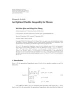
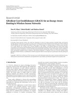
Figure 1: Three sampled TSs with different shapes.
Table 1: SimilB, the ED, the CC between f

2
and f
1
,and f
2
and f
3
in
Figure 1.
TSs ED CC SimilB

f
2
, f
1

3.9955 0.0917 0.930

f
2
, f
3

3.9955 0.0917 0.750
Table 2: Classification errors of clustering task using the SimilB, the
ED, and the CC for CBF.dat dataset.
SimilB ED CC
0.222 0.888 0.888
form of the operator noted Ψ
B

d
and operating on discrete-
time signals x(n)andy(n). Three sample differences are ex-
amined. For simplicity, we replace t by nT
s
(T
s
is the sam-
pling period), x(t)withx(nT
s
) or simply x(n). Using the
same reasoning as in [8] we obtain the following relations.
(i) Two-sample backward difference:
˙
x(t)
−→

x
k
(n) −x
k
(n −1)

T
s
,
¨
x(t)
−→


x
k
(n) −2x
k
(n −1) + x
k
(n −2)

T
2
s
,
Ψ
B
(x
k
(t), y
k
(t)) −→
x
k
(n −1)y
k
(n −1)
T
2
s
−
0.5


x
k
(n)y
k
(n −2) + y
k
(n)x
k
(n −2)

T
2
s
,
Ψ
B

x
k
(t), y
k
(t)

−→
Ψ
B
d

x
k

(n −1), y
k
(n −1)

T
2
s
, k ∈{i, r}.
(5)
Abdel-Ouahab Boudraa et al. 3
Table 3: Estimated T
B
value versus SNR signals s
1
(t)ands
2
(t) using SimilB.
SimilB SNR = −6 dB SNR = −2 dB SNR = 1 dB SNR = 3 dB SNR = 5 dB SNR = 9dB

s
1
(t),r
1
(t)

300 ±1 300 ±1 300 300 300 300

s
2
(t),r

2
(t)

300 ±2 300 ±1 300 ± 1 300 ±1 300 ±1 300
Finally, the discrete form of Ψ
B
(x(t), y(t)) is given by
Ψ
B

x(t), y(t)

−→

Ψ
B
d

x
r
(n−1), y
r
(n−1)

+ Ψ
B
d

x
i

(n−1), y
i
(n−1)

T
2
s
,
(6)
where
−→ denotes the mapping from continuous to discrete.
(ii) Two-sample forward difference:
˙
x(t)
−→

x
k
(n +1)− x
k
(n)

T
s
,
¨
x(t)
−→

x

k
(n +2)− 2x
k
(n +1)+x
k
(n)

T
2
s
,
Ψ
B

x
k
(t), y
k
(t)

−→
x
k
(n +1)y
k
(n +1)
T
2
s
−

0.5

x
k
(n +2)y
k
(n)+y
k
(n +2)x
k
(n)

T
2
s
,
Ψ
B

x
k
(t), y
k
(t)

−→
Ψ
B
d


x
k
(n +1),y
k
(n +1)

T
2
s
, k ∈{i, r}.
(7)
Thus, from Ψ
B
we obtain Ψ
B
d
shiftedbyonesampleto
the right and scaled by T
−2
s
. Finally, the discrete form of
Ψ
B
(x(t), y(t)) is given by
Ψ
B

x(t), y(t)

−→


Ψ
B
d

x
r
(n +1), y
r
(n +1)

+ Ψ
B
d

x
i
(n +1), y
i
(n +1)

T
2
s
.
(8)
Note that for both asymmetric two-sample differences, Ψ
B
is shifted by one sample and scaled by T
−2

s
. If we ignore the
one-sample shift and the scaling parameter, one can trans-
form Ψ
B
(x(t), y(t)) into Ψ
B
d
(x(n), y(n)) as follows:
Ψ
B

x(t), y(t)

−→
Ψ
B
d

x
r
(n), y
r
(n)

+ Ψ
B
d

x

i
(n), y
i
(n)

,
(9)
Ψ
B
d

x
k
(n), y
k
(n)

=
x
k
(n)y
k
(n) −0.5

x
k
(n +1)y
k
(n −1)
+ y

k
(n +1)x
k
(n −1)

, k ∈{i, r}.
(10)
0 20 40 60 80 100 120 140
Time
−5
0
5
10
Amplitude
Cylinder
(a)
0 20 40 60 80 100 120 140
Time
−5
0
5
10
Amplitude
Bell
(b)
0 20 40 60 80 100 120 140
Time
−5
0
5

10
Amplitude
Funnel
(c)
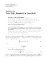
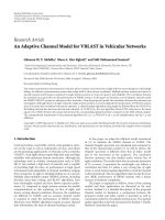
Figure 2: The Cylinder-Bell-Funnel dataset (CBF.dat) [10].
(iii) Three-sample symmetric difference:
˙
x(t)
−→

x
k
(n +1)− x
k
(n −1)

2T
s
,
¨
x(t)
−→

x
k
(n +2)− 2x
k
(n)+x
k
(n −2)


4T
2
s
,
Ψ
B

x
k
(t), y
k
(t)

−→
2x
k
(n)y
k
(n)
4T
2
s
−

x
k
(n+1)y
k
(n−1)+y

k
(n+1)x
k
(n−1)

4T
2
s
,
x
k
(n−1)y
k
(n−1)
4T
2
s
−
0.5

x
k
(n)y
k
(n−2) + y
k
(n)x
k
(n−2)


4T
2
s
+
x
k
(n+1)y
k
(n+1)
4T
2
s
−
0.5

x
k
(n+2)y
k
(n)+y
k
(n +2)x
k
(n)

4T
2
s
,
Ψ

B

x
k
(t), y
k
(t)

−→

Ψ
B
d

x
k
(n+1), y
k
(n+1)

+2Ψ
B
d

x
k
(n), y
k
(n)


+Ψ
B
d

x
k
(n −1), y
k
(n −1)

/4T
2
s
, k ∈{i, r}.
(11)
4 EURASIP Journal on Advances in Signal Processing
172589364
Labels
12
14
16
18
20
22
24
26
28
30
32
Threshold

Euclidean
(a)
172589364
Labels
0.2
0.3
0.4
0.5
0.6
0.7
0.8
0.9
1
Threshold
Correlation
(b)
123456789
Labels
300
350
400
450
500
550
Threshold
SimilB
(c)
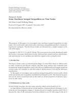
Figure 3: Comparison of the SimilB, the ED, the CC on a clustering task. Labels (1,2,3), (4,5,6), and (7,8,9) correspond to Cylinder, Bell,
and Funnel classes, respectively.
Compared to asymmetric two-sample differences, the three-

sample symmetric difference leads to more complicated
expression. Expression (11) corresponds to three-sample
weighted moving average of Ψ
B
d
(x
k
(n), y
k
(n)). Note if x =
y, Ψ
B
d
is reduced to the Teager-Kaiser operator (TKO):
Ψ
B
d
(x(n),x(n)) = x
2
(n) −x(n +1)x(n −1) (see [9]). Finally,
the asymmetric approximation is less complicated for imple-
mentation and is faster than the symmetric one.
5. PROPERTIES OF Ψ
B
WeprovideheresomenewpropertiesofΨ
B
[1]. We denote
Ψ
B
of x(t)andy(t)byΨ

B
(x, y; t) and denote by “← ” the
affectation operation.
Similarity measure:
Ψ
B
(x, y; t) = Ψ
B
(y, x; t). (12)
This is a basic requirement for most of similarity or distance
measures.
Time shift:
x
1
(t) ←− x

t −t
0

,
y
1
(t) ←− y

t −t
0

.
(13)
It is trivial that Ψ

B
is time-shift invariant, that is,
Ψ
B
(x
1
, y
1
; t) = Ψ
B
(x, y; t −t
0
). This property states that any
time translations in the signals, x(t)andy(t), should be
preserved in their measure of interaction, Ψ
B
(x, y; t). Thus,
Ψ
B
(x, y; t) is robust to time shifts.
Amplitude scale:
x
1
(t) ←− α·x(t),
y
1
(t) ←− β·y(t).
(14)
It is easy to verify that Ψ
B

(x
1
, y
1
; t) = α·βΨ
B
(x, y; t). Thus,
the time where Ψ
B
peaks, corresponding to the maximum
of interaction between x(t)andy(t), is robust to amplitude
scale.
Time scale:
x
1
(t) ←− x(at),
y
1
(t) ←− y(at).
(15)
It is easy to verify that Ψ
B
(x
1
, y
1
; t) = a
2
Ψ
B

(x, y; t). This
property states that if the time of the two signals is com-
pressed by a scale a, then the energy of interaction is com-
pressed by a
2
.
Abdel-Ouahab Boudraa et al. 5
0 50 100 150 200
Times
−1
−0.5
0
0.5
1
Signal X
(a)
0 50 100 150 200
Times
0.05
0.1
0.15
0.2
0.25
Normalized frequency
Signal X
Intersection frequency
(b)
0 50 100 150 200
Times
−1

−0.5
0
0.5
1
Signal Y
(c)
0 50 100 150 200
Times
0.05
0.1
0.15
0.2
0.25
Normalized frequency
Signal Y
Intersection frequency
(d)
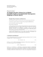
Figure 4: Linear chirp TSs (parabolic phase).
0 50 100 150 200
Times
0
0.2
0.4
0.6
0.8
1
1.2
1.4
1.6
1.8

Amplitude
Ψ (Y, Y) Ψ (X,X)
Ψ
(X, Y)
Intersection frequency
Figure 5: Similarity measure using SimilB with a sliding window
analysis.
5.1. Ψ
B
-based similarity measure
A similarity measure S(x(t), y(t)) is a function to compare
the TSs x(t)andy(t). Conventionally, this measure is a
0 50 100 150 200
Time
−0.2
−0.15
−0.1
−0.05
0
0.05
0.1
0.15
Amplitude
Figure 6: Similarity measure using CC with a sliding window anal-
ysis.
symmetric function whose value is large when x and y are
somehow similar. The proposed similarity measure based on
Ψ
B
(x, y), between x(t)andy(t), uses their interaction. A

6 EURASIP Journal on Advances in Signal Processing
0 50 100 150 200 250 300 350 400 450 500
Time
0 50 100 150 200 250 300 350 400 450 500
−2
0
2
4
6
Amplitude
−1
−0.5
0
0.5
1
Amplitude
s
2
(t)
s
1
(t)
(a) Signals s
1
(t)ands
2
(t)
0 50 100 150 200 250 300 350 400 450 500
Time
−500

−400
−300
−200
−100
0
100
200
300
400
500
Amplitude
CC
(b) CC with a sliding window analysis
0 50 100 150 200 250 300 350 400 450 500
Time
0
0.1
0.2
0.3
0.4
0.5
0.6
0.7
0.8
0.9
1
Amplitude
SimilB
(c) SimilB with a sliding window analysis
Figure 7: Similarity measure using SimilB and CC of sinusoidal TSs.

larger value indicates more interaction in energy between
TSs. If the input variables (or samples) of the TS x(t)(or
y(t)) have large range, then this can overpower the other in-
put variables of y(t)(orx(t)). Therefore, the proposed sim-
ilarity measure, SimilB, is a normalized version of Ψ
B
(x, y)
andisdefinedasfollows:
SimilB(x, y)
=
√
2

T
Ψ
B
(x, y)dt

T

Ψ
2
B
(x,x)+Ψ
2
B
(y, y)dt
. (16)
T is the TS duration or the size of sliding window analysis.
The similarity is symmetric when comparing two TSs:

SimilB(x, y)
= SimilB(y, x) ∀(x, y) ∈ C
2
. (17)
It is a basic requirement for most of similarity or distance
measures. Note that if x
= y then SimilB(x, y) = 1.
6. RESULTS
SimilB (equation (17)) is combined with relations (10)and
(11), and relation (3)or(4) to process discrete (Figure 2)and
continuous (Figures 1, 4, 7,and8) data, respectively. The ef-
fects of temporal information and the inclusion of the signal
derivatives are shown on nonstationary and stationary syn-
thetic TSs. Figure 1 shows three TSs with different shapes to
illustrate the limit of the ED and the CC. Since f
1
, f
2
,and f
3
have different shapes, then an appropriate similarity measure
would show, for example, that the similarity values between
f
1
and f
2
and that between f
3
and f
2

are different. Results of
the SimilB, the ED, and the CC between f
2
and f
1
and that
between f
2
and f
3
are reported in Table 1 . These results show
that SimilB is the unique measure which properly capture
the temporal information in the comparison of the shapes.
The most studied TS classification/clustering problem is the
Cylinder-Bell-Funnel dataset (noted CBF.dat) [10]. It is a 3-
class problem. Typical examples of each class are shown in
Figure 2. The classes are generated by the equations [10]
c(t)
= (6 + η)·X
[a,b]
(t)+(t) // Cylinder class,
b(t)
= (6 + η)·X
[a,b]
(t).
(t
−a)
(b − a)
+
(t) // Bell class,

f (t)
= (6 + η)·X
[a,b]
(t).
(b
−t)
(b − a)
+
(t) // Funnel class,
X
[a,b]
= 1ifa ≤ t ≤ b, else X
[a,b]
= 0,
(18)
where η and
(t) are drawn from a standard normal distribu-
tion N (0,1), a is an integer drawn uniformly from the range
[16, 32], and (b
− a) is an integer drawn uniformly from the
range [32, 96] (Figure 2).ThetaskistoclassifyaTSasone
of the three classes, Cylinder, Bell, or Funnel. We have per-
formed an experiment classification on CBF.dat dataset con-
sisting of 3 TSs of each class. TSs are clustered using group-
average hierarchical clustering. The dendrograms are formed
with nearest neighbor linkage for three of each type of TSs
using SimilB measure, the ED, and the CC. We have averaged
Abdel-Ouahab Boudraa et al. 7
0204060
Time

0
0.5
1
s
1
(t)
(a)
020406080
Time
−1
0
1
s
2
(t)
(d)
0 200 400 600
Time
−1
0
1
r
1
(t)
(b)
0 200 400 600
Time
−1
0
1

r
2
(t)
(e)
0 200 400 600
Time
−0.5
0
0.5
1
(s
1
(t), r
1
(t))
T
(c)
0 200 400 600
Time
−1
0
1
(s
2
(t), r
2
(t))
T
(f)
Figure 8: Similarity measure using SimilB of TSs of nonequal length.

the classification results over 45 runs. Figure 3 shows the re-
sult of these averaged runs where both the ED and the CC
fail to differentiate between the three classes. SimilB distin-
guishes the three original classes as shown in Figure 3. Clas-
sification errors reported in Ta ble 2 show that SimilB is more
effective than the ED and the CC. These results are expected
since the ED and the CC are not able to include the tempo-
ral information while SimilB using derivatives of the TS cap-
tures this kind of information. Moreover, these results may
be due to the fact that Ψ
B
is local operator [1, 6] while the
ED and the CC are global ones. Figure 4 shows an exam-
ple of nonstationary TSs (two linear FM signals), x(t)and
y(t). The instantaneous frequency (IF) of x(t) increases lin-
early with time while that of y(t) decreases with time. The
point where the IFs intercept (Figure 4), noted Q,islocated
at t
= 125. Figure 5 shows the energy of each TS and the en-
ergy of their interaction obtained with a sliding window anal-
ysis of T
= 15. The point Q corresponds to the maximum
of similarity and also where the energy of x(t) (SimilB(x,x))
and that of y(t) (SimilB(y, y)) are equal. Away from Q, the
amplitude of interaction decreases because there is less sim-
ilarity between TSs (the TSs tend to be more and more dif-
ferent). As the IFs converge from the time origin to Q (the
TSs tend to be equal), the interaction intensity of the TSs in-
creases and the maximum of similarity is achieved at t
= 125.

Figure 6 shows that the maximum of similarity given by CC
is located at t
= 240. Thus, the CC fails to point out, as ex-
pected (Figure 4), the maximum of similarity at Q. The in-
teraction measure using SimilB and CC is performed using
a sliding window analysis of size T.Different T values rang-
ing from 3 to 91 have been tested. Globally, we found com-
parable results. The CC is calculated with the same sliding
window as for SimilB. Furthermore, as the IFs converge to Q
or diverge from Q, the CC function has, globally, the same
behavior and thus the similarity study of such TSs is diffi-
cult. This example shows that the SimilB is more effective
to study nonstationary TSs than the CC. This may be due
the fact that the Ψ
B
is nonlinear operator while the CC is
linear one. Figure 7(a) shows an example of two sinusoidal
TSs, s
1
(t)ands
2
(t), of the same frequency and amplitude. TS
s
2
(t) presents a discontinuity located at t = 200. Both CC
and SimilB are calculated with T set to 17. CC measure fails
to detect the discontinuity and shows a maximum of interac-
tion at t
= 262 (Figure 7(b)). The result of SimilB is expected
(Figure 7(c)). Indeed, excepted for data point at t

= 200, s
1
(t)
and s
2
(t)areequalandΨ
B
behaves toward these two signals
as the TKO applied to s
1
(t)(s
2
(t)) and thus giving a constant
output (square of the amplitude times the frequency) [9].
This example shows the interest of SimilB to track disconti-
nuities (Figure 7(c)). Two synthetic signals, s
1
(t)ands
2
(t), of
8 EURASIP Journal on Advances in Signal Processing
nonequal lengths with size window observation T of 65 and
81, respectively, are shown in Figures 8(a) and 8(d). These
two signals are time shifted by 300 samples and corrupted
by additive Gaussian noise. The obtained signals, r
1
(t)and
r
2
(t), are shown in Figures 8(b) and 8(e), respectively. The

attenuation coefficient is set to 0.7. For both signals r
1
(t)and
r
2
(t), a similarity measure would show, in theory, a maxi-
mum of interaction located at t
= 300. No warping pro-
cess is used. We use the smallest TS length as a sliding win-
dow and calculate SimilB, inside this window, between two
TSs of the same length. Outputs of SimilB are shown in Fig-
ures 8(c) and 8(f) indicating a net maximum at t
= T
B
.
As expected, both SimilB(s
1
(t), r
1
(t)) and SimilB(s
2
(t),r
2
(t))
peak to T
B
= 300. Ta ble 3 lists the T
B
values calculated for
SimilB(s

1
(t), r
1
(t)) and SimilB(s
2
(t), r
2
(t)) for different SNRs
ranging from
−6dBto9dB.EachvalueofTa ble 3 corre-
sponds to the average of an ensemble of twenty five trials of
T
B
estimation. These results show that the performances of
SimilB are very close to that of the theory and also that SimilB
works correctly for moderately noisy TSs.
7. CONCLUSION
Relative change of amplitude and the corresponding tempo-
ral information are well suited to measure similarity between
TSs. In this paper, a new nonlinear similarity measure for TS
analysis, SimilB, which takes into account the temporal in-
formation is introduced. Using the first and second deriva-
tives of the TS, SimilB is able to capture temporal changes
and discontinuities of the TS. Some new properties of Ψ
B
are presented showing, particularly, that the interaction mea-
sure is robust both to time shift and amplitude scale. It is also
shown that if the time of the signals is scaled by a factor, the
corresponding interaction energy is proportional to that of
the original ones. Thus, the time corresponding to the max-

imum of interaction is unchanged by time scale. Note that
SimilB is not a unique measure of similarity based on Ψ
B
op-
erator. Different similarity based on Ψ
B
can be constructed.
To process continuous analytic TSs an expression of Ψ
B
is
provided. The discrete version of Ψ
B
, for its implementation,
is presented and three derivative approximations are exam-
ined. Only the asymmetric approximation which is less com-
plicated and less time consuming is implemented. Results of
different synthetic TSs (stationary and nonstationary) show
that SimilB performs better than the ED and the CC and
show the interest to take into account the relative changes
of the TSs. Compared to generative models (HMM, GMM,
) or distance kernel-based methods, SimilB is nonpara-
metric approach that does not require the specification of a
kernel or the selection of a probability distribution. Further-
more, SimilB is fast and easy to implement. SimilB may be
viewed as a data-driven approach because no a priori infor-
mation about the signals or parameters setting is required.
The processed TSs are either noiseless or moderately noisy.
For very noisy TSs, the robustness of SimilB must be studied.
In a future work, we plan to use smooth splines to give more
robustness to SimilB [11]. We also plan to include the Sim-

ilB measure in a clustering process or algorithm such as fuzzy
c-means or k-means for classification of TSs in different clus-
ters. To confirm the presented results, a large class of real TSs
datasets must be studied as well as the results compared to
other methods particularly those including the temporal in-
formation.
REFERENCES
[1] J C. Cexus and A O. Boudraa, “Link between cross-Wigner
distribution and cross-Teager energy operator,” Electronics Let-
ters, vol. 40, no. 12, pp. 778–780, 2004.
[2] J. Alon, S. Sclaroff, G. Kollios, and V. Pavlovic, “Discovering
clusters in motion time-series data,” in Proceedings of IEEE
Computer Society Conference on Computer Vision and Pattern
Recognition (CVPR ’03), vol. 1, pp. 375–381, Madison, Wis,
USA, June 2003.
[3] R. Agrawal, C. Faloutsos, and A. Swami, “Efficient similarity
search in sequence databases,” in Proceedings of the 4th Inter-
national Conference on Foundations of Data Organization and
Algorithms (FODO ’93), vol. 730 of Lecture Notes in Computer
Science, pp. 69–84, Chicago, Ill, USA, October 1993.
[4] S.Chu,E.Keogh,D.Hart,andM.Pezzani,“Iterativedeepen-
ing dynamic time warping for time series,” in Proceedings of the
2nd SIAM International Conference on Data Mining, Arlington,
Va, USA, April 2002.
[5]C.S.M
¨
oller-Levet, F. Klawonn, K. H. Cho, and O. Wolken-
hauer, “Fuzzy clustering of short time-series and unevenly
distributed sampling points,” in Proceedings of the 5th Inter-
national Symposium on Intelligent Data Analysis (IDA ’03),

vol. 2810 of Lecture Notes in Computer Science, pp. 330–340,
Berlin, Germany, August 2003.
[6] Z. Saidi, A O. Boudraa, J C. Cexus, and S. Bourennane,
“Time-delay estimation using cross-Ψ
B
-energy operator,” In-
ternational Journal of Signal Processing, vol. 1, no. 1, pp. 28–32,
2004.
[7] P. Maragos and A. Potamianos, “Higher order differential en-
ergy operators,” IEEE Signal Processing Letters, vol. 2, no. 8, pp.
152–154, 1995.
[8] P. Maragos, J. F. Kaiser, and T. F. Quatieri, “On amplitude
and frequency demodulation using energy operators,” IEEE
Transactions on Signal Processing, vol. 41, no. 4, pp. 1532–1550,
1993.
[9] J. F. Kaiser, “Some useful properties of Teager’s energy opera-
tors,” in Proceedings of IEEE International Conference on Acous-
tics, Speech, and Signal Processing (ICASSP ’93), vol. 3, pp. 149–
152, Minneapolis, Minn, USA, April 1993.
[10] N. Saito, Local feature extraction and its application using a li-
brary of bases, Ph.D. thesis, Yale University, New Haven, Conn,
USA, 1994.
[11] D. Dimitriadis and P. Maragos, “An improved energy demod-
ulation algorithm using splines,” in Proceedings of IEEE Inter-
national Conference on Acoustics, Speech, and Signal Process-
ing (ICASSP ’01), vol. 6, pp. 3481–3484, Salt Lake, Utah, USA,
May 2001.