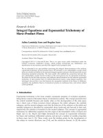
Báo cáo hóa học: " Research Article Downsampling Non-Uniformly Sampled Data" potx

Hindawi Publishing Corporation
EURASIP Journal on Advances in Signal Processing
Volume 2008, Article ID 147407, 10 pages
doi:10.1155/2008/147407
Research Article
Downsampling Non-Uniformly Sampled Data
Frida Eng and Fredrik Gustafsson
Department of Electrical Engineering, Link
¨
opings Universitet, 58183 Link
¨
oping, Sweden
Correspondence should be addressed to Fredrik Gustafsson,
Received 14 February 2007; Accepted 17 July 2007
Recommended by T H. Li
Decimating a uniformly sampled signal a factor D involves low-pass antialias filtering with normalized cutoff frequency 1/D
followed by picking out every Dth sample. Alternatively, decimation can be done in the frequency domain using the fast Fourier
transform (FFT) algorithm, after zero-padding the signal and truncating the FFT. We outline three approaches to decimate non-
uniformly sampled signals, which are all based on interpolation. The interpolation is done in different domains, and the inter-
sample behavior does not need to be known. The first one interpolates the signal to a uniformly sampling, after which standard
decimation can be applied. The second one interpolates a continuous-time convolution integral, that implements the antialias
filter, after which every Dth sample can be picked out. The third frequency domain approach computes an approximate Fourier
transform, after which truncation and IFFT give the desired result. Simulations indicate that the second approach is particularly
useful. A thorough analysis is therefore performed for this case, using the assumption that the non-uniformly distributed sampling
instants are generated by a stochastic process.
Copyright © 2008 F. Eng and F. Gustafsson. This is an open access article distributed under the Creative Commons Attribution
License, which permits unrestricted use, distribution, and reproduction in any medium, provided the original work is properly
cited.
1. INTRODUCTION
Downsampling is here considered for a non-uniformly sam-
pled signal. Non-uniform sampling appears in many applica-

tions, while the cause for nonlinear sampling can be classified
into one of the following two categories.
Event-based sampling
The sampling is determined by a nuisance event process. One
typical example is data traffic in the Internet, where packet
arrivals determine the sampling times and the queue length
is the signal to be analyzed. Financial data, where the stock
market valuations are determined by each transaction, is an-
other example.
Uniform sampling in secondary domain
Some angular speed sensors give a pulse each time the shaft
has passed a certain angle, so the sampling times depend on
angular speed. Also biological signals such as ECGs are natu-
rally sampled in the time domain, but preferably analyzed in
another domain (heart rate domain).
A number of other applications and relevant references
can be found in, for example, [1].
It should be obvious from the examples above that for
most applications, the original non-uniformly sampled sig-
nal is sampled much too fast, and that oscillation modes and
interesting frequency modes are found at quite low frequen-
cies compared to the inverse mean sampling interval.
The problem at hand is stated as follows.
Problem 1. The following is given:
(a) a sequence of non-uniform sampling times, t
m
, m =
1, , M;
(b) corresponding signal samples, u(t
m

);
(c) a filter impulse response, h(t); and
(d) a resampling frequency, 1/T.
Also, the desired intersampling time, T, is much larger than
the original mean intersampling time,
μ
T
 E

t
m
− t
m−1

≈
t
M
M
= T
u
. (1)
2 EURASIP Journal on Advances in Signal Processing
Let x denote the largest integer smaller than or equal to
x. Find
z(nT), n = 1, , N,
N
=

t
M

T


M
D
,
(2)
such that
z(nT) approximates z(nT), where
z(t)
= h  u(t) =

h(t −τ)u(τ)dτ (3)
is given by convolution of the continuous-time filter h(t)and
signal u(t).
For the case of uniform sampling, t
m
= mT
u
,twowell-
known solutions exist; see, for example, [2].
(a) First, if T/T
u
= D is an integer, then (i) u(mT
u
)isfil-
tered giving z(mT
u
), and (ii) z(nT) = z(nDT
u

)gives
the decimated signal.
(b) Further, if T/T
u
= R/S is a rational number, then a
frequency domain method is known. It is based on
(i) zero padding u(mT
u
)tolengthRM, (ii) computing
the discrete Fourier transform (DFT), (iii) truncating
the DFT a factor S, and finally computing the inverse
DFT (IDFT), where the (I)FFT algorithm is used for
the (I)DFT calculation.
Conversion between arbitrary sampling rates has also
been discussed in many contexts. The issues with efficient
implementation of the algorithms are investigated in [3–
6], and some of the results are beneficial also for the non-
uniform case.
Resampling and reconstruction are closely connected,
since a reconstructed signal can be used to sample at desired
timepoints.Thetaskofreconstructioniswellinvestigated
for different setups of non-uniform sampling. A number of
iterative solutions have been proposed, for example, [1, 7, 8],
several more are also discussed in [9]. The algorithms are
not well-suited for real-time implementations and are based
on different assumptions on the sampling times, t
m
,suchas
bounds on the maximum separation or deviation from the
nominal value mT

u
.
Russel [9] also investigates both uniform and non-
uniform resampling thoroughly. Russell argues against the
iterative solutions, since they are based on analysis with ideal
filters, and no guarantees can be given for approximate so-
lutions. A noniternative approach is given, which assumes
periodic time grids, that is, the non-uniformity is repeated.
Another overview of techniques for non-uniform sampling
is given in [10], where, for example, Ferreira [11] studies the
special case of recovery of missing data and Lacaze [12]re-
constructs stationary processes.
Reconstruction of functions with a convolutional ap-
proach was done by [13], and later also by [14]. The sampling
is done via basis functions, and reduces to the regular case if
delta functions are used. These works are based on sampling
sets that fulfill the non-uniform sampling theorem given in
[15].
Reconstruction has long been an interesting topic in im-
age processing, especially in medical imaging, see, for exam-
ple, [16], where, in particular, problems with motion arti-
facts are addressed. Arbitrary sampling distributions are al-
lowed, and the reconstruction is done through resampling
to a uniform grid. The missing pixel problem is given at-
tention in [9, 17]. In [18], approximation of a function with
bounded variation, with a band-limited function, is consid-
ered and the approximation error is derived. Pointwise re-
construction is investigated in [19], and these results will be
used in Section 5.
Here, we neither put any constraints on the non-uniform

sampling times, nor assumptions on the signal’s function
class. Instead, we take a more application-oriented approach,
and aim at good, implementable, resampling procedures. We
will consider three different methods for converting from
non-uniform to uniform sampling. The first and third al-
gorithm are rather trivial modifications of the time and
frequency-domain methods for uniformly sampled data, re-
spectively, while the second one is a new truly non-uniform
algorithm. We will compare performance of these three. In
all three cases, different kinds of interpolation are possible,
but we will focus on zero-order hold (nearest neighbor) and
first order hold (linear interpolation). Of course, which in-
terpolation is best depends on the signal and in particular
on its inter-sample behavior. Though we prefer to talk about
decimation, we want to point out that the theories hold for
any type of filter h(t).
A major contribution in this work is a detailed analysis of
the algorithms, where we assume additive random sampling,
(ARS),
t
m
= t
m−1
+ τ
m
,(4)
where τ
m
is stochastic additive sampling noise given by the
known probability density function p

τ
(t). The theoretical re-
sults show that the downsampled signal is unbiased under
fairly general conditions and present an equivalent filter that
generates z(t)
=

h  u(t), where

h depends on the designed
filter h and the characteristic function of the stochastic dis-
tribution.
The paper is organized as follows. The algorithms are de-
scribed in Section 2. The convolutional interpolation gives
promising results in the simulations in Section 3, and the last
sections are dedicated to this algorithm. In Section 4, theo-
retic analysis of both finite time and asymptotic performance
is done. The section also includes illustrative examples of the
theory. Section 5 investigates an application example and is-
sues with choosing the filter h(t), while Section 6 concludes
the paper.
2. INTERPOLATION ALGORITHMS
Time-domain interpolation can be used with subsequent fil-
tering. Since LP-filtering is desired, we also propose two other
methods that include the filter action directly. The main idea
is to perform the interpolation at different levels and the
problem was stated in Problem 1.
F. Eng and F. Gustafsson 3
For Problem 1, with T
u

= t
M
/M,compute
(1) t
j
m
= arg min
t
m
<jT
u
|jT
u
− t
m
|,
(2)
u(jT
u
) = u(t
j
m
),
(3)
z(kT) =
M

j=1
h
d

(kT − jT
u
)u(jT
u
),
where h
d
(t) is a discrete time realization of
the impulse response h(t).
Algorithm 1: Time-domain interpolation.
2.1. Interpolation in time domain
It is well described in literature how to interpolate a signal or
function in, for instance, the following cases.
(i) The signal is band-limited, in which case the sinc in-
terpolation kernel gives a reconstruction with no error
[20].
(ii) The signal has vanishing derivatives of order n +1and
higher, in which case spline interpolation of order n is
optimal [21].
(iii) The signal has a bounded second-order derivative, in
which case the Epanechnikov kernel is the optimal in-
terpolation kernel [19].
The computation burden in the first case is a limiting fac-
tor in applications, and for the other two examples, the inter-
polation is not exact. We consider a simple spline interpola-
tion, followed by filtering and decimation as in Algorithm 1.
This is a slight modification of the known solution in the uni-
form case as was mentioned in Section 1.
Algorithm 1 is optimal only in the unrealistic case where
the underlying signal u(t) is piecewise constant between the

samples. The error will depend on the relation between the
original and the wanted sampling; the larger the ratio M/N,
the smaller the error. If one assumes a band-limited signal,
where all energy of the Fourier transform U( f )isrestricted
to f<0.5N/t
M
, then a perfect reconstruction would be pos-
sible, after which any type of filtering and sampling can be
performed without error. However, this is not a feasible so-
lution in practice, and the band-limited assumption is not
satisfied for real signals when the sensor is affected by addi-
tive noise.
Remark 1. Algorithm 1 finds
u(jT
u
) by zero-order hold in-
terpolation, where of course linear interpolation or higher-
order splines could be used. However, simulations not in-
cluded showed that this choice does not significantly affect
the performance.
2.2. Interpolation in the convolution integral
Filtering of the continuous-time signal, u, yields
z(kT)
=

h(kT − τ)u(τ)dτ,(5)
For Problem 1,compute
(1)
z(kT) =
M


m=1
τ
m
h(kT − t
m
)u(t
m
).
Algorithm 2: Convolution interpolation.
and using Riemann integration, we get Algorithm 2. The al-
gorithm will be exact if the integrand, h(kT
−τ)u(τ), is con-
stant between the sampling points, t
m
,forallkT. As stated
before, the error, when this is not the case, decreases when
the ratio M/N increases.
This algorithm can be further analyzed using the inverse
Fourier transform, and the results in [22], which will be done
in Section 4.1.
Remark 2. Higher-order interpolations of (5) were studied
in [23] without finding any benefits.
When the filter h(t) is causal, the summation is only
taken over m such that t
m
<kT,andthusAlgorithm 2 is
ready for online use.
2.3. Interpolation in the frequency domain
LP-filtering is given by a multiplication in the frequency do-

main, and we can form the approximate Fourier transform
(AFT), [22], given by Riemann integration of the Fourier
transform, to get Algorithm 3. This is also a known approach
in the uniform sampling case, where the DFT is used in each
step. The AFT is formed for 2N frequencies to avoid circular
convolution. This corresponds to zero-padding for uniform
sampling. Then the inverse DFT gives the estimate.
Remark 3. The AFT used in Algorithm 3 is based on Rie-
mann integration of the Fourier transform of u(t), and
would be exact whenever u(t)e
−i2πft
is constant between
sampling times, which of course is rarely the case. As for the
two previous algorithms, the approximation is less grave for
large enough M/N. This paper does not include an investiga-
tion of error bounds.
More investigations of the AFT were done in [22].
2.4. Complexity
In applications, implementation complexity is often an issue.
We calculate the number of operations, N
op
, in terms of addi-
tions (a), multiplications (m), and exponentials (e). As stated
before, we have M measurements at non-uniform times, and
want the signal value at N time points, equally spaced with
T.
(i) Step (3) in Algorithm 1 is a linear filter, with one addi-
tion and one multiplication in each term,
N
1

op
= (1m +1a)MN. (6)
4 EURASIP Journal on Advances in Signal Processing
For Problem 1,compute
(1) f
n
= n/2NT, n = 0, ,2N − 1,
(2)

U( f
n
) =
M

m=1
τ
m
u(t
m
)e
−i2πf
n
t
m
, n = 0, , N,
(3)

Z( f
n
) =


Z( f
2N−n
)

= H( f
n
)

U( f
n
),
n
= 0, ,N,
(4)
z(kT) = 1/2NT
2N−1

n=0

Z( f
n
)e
i2πkT f
n
k = 0, , N − 1.
Here,

Z


is the complex conjugate of

Z.
Algorithm 3: Frequency-domain interpolation.
Computing the convolution in step (3) in the fre-
quency domain would require the order of M log
2
(M)
operations.
(ii) Algorithm 2 is similar to Algorithm 1,
N
2
op
= (2m +1a)MN,(7)
where the extra multiplication comes from the factor
τ
m
.
(iii) Algorithm 3 performs an AFT in step (2), frequency-
domain filtering in step (3) and an IDFT in step (4),
N
3
op
= (2m +le +la)2M(N +1)
+(lm)(N +1)
+(le +lm +la)2N
2
.
(8)
Using the IFFT algorithm in step (4) would give

Nlog
2
(2N) instead, but the major part is still MN.
All three algorithms are thus of the order MN, though Algo-
rithms 1 and 2 have smaller constants.
Studying work on efficient implementation, for example,
[9], performance improvements, could be made also here,
mainly for Algorithms 1 and 2, where the setup is similar.
Taking the length of the filter h(t) into account can sig-
nificantly improve the implementation speed. If the impulse
response is short, the number of terms in the sums in Algo-
rithms 1 and 2 will be reduced, as well as the number of extra
frequencies needed in Algorithm 3.
3. NUMERIC EVALUATION
We will use the following example to test the performance of
these algorithms. The signal consists of three frequencies that
are drawn randomly for each test run.
Example 1. A signal with three frequencies, f
j
,drawnfroma
rectangular distribution, Re, is simulated
s(t)
= sin

2πf
1
t −1

+sin


2πf
2
t −1

+sin

2πf
3
t

,(9)
f
j
∈ Re

0.01,
1
2T

, j = 1, 2,3. (10)
The desired uniform sampling is given by the intersampling
time T
= 4 seconds. The non-uniform sampling is defined
by
t
m
= t
m−1
+ τ
m

, (11)
τ
m
∈ Re(t
l
, t
h
), (12)
and the limits t
l
and t
h
are varied. In the simulation, N is set
to 64 and the number of non-uniform samples are chosen so
that t
M
>NTis assured. This is not in exact correspondence
with the problem formulation, but assures that the results for
different τ
m
-distributions are comparable.
The samples are corrupted by additive measurement
noise,
u

t
m

=
s


t
m

+ e

t
m

, (13)
where e(t
m
) ∈ N(0, σ
2
), σ
2
= 0.1.
The filter is a second-order LP-filter of Butterworth type
with cutoff frequency 1/2T, that is,
h(t)
=
√
2
π
T
e
−(π/T
√
2)t
sin


π
T
√
2
t

, t>0, (14)
H(s)
=
(π/T)
2
s
2
+
√
2π/Ts +(π/T)
2
. (15)
This setup is used for 500 different realizations of f
j
, τ
m
,
and e(t
m
).
We w il l te st fo ur d ifferent rectangular distributions (12):
τ
m

∈ Re(0.1, 0.3), μ
T
= 0.2, σ
T
= 0.06, (16a)
τ
m
∈ Re(0.3, 0.5), μ
T
= 0.4, σ
T
= 0.06, (16b)
τ
m
∈ Re(0.4, 0.6), μ
T
= 0.5, σ
T
= 0.06, (16c)
τ
m
∈ Re(0.2, 0.6), μ
T
= 0.4, σ
T
= 0.12, (16d)
and the mean values, μ
T
, and standard deviations, σ
T

,are
shown for reference. For every run, we use the algorithms
presented in the previous section and compare their results
to the exact, continuous-time, result,
z(kT)
=

h(kT − τ)s(τ)dτ. (17)
We calculate the root mean square error, RMSE,
λ 




1
N

k


z(kT) − z(kT)


2
. (18)
The algorithms are ordered according to lowest RMSE, (18),
and Ta bl e 1 presents the result. The number of first, second
and third positions for each algorithm during the 500 runs,
are also presented. Figure 1 presents one example of the re-
sult, though the algorithms are hard to be separated by visual

inspection.
A number of conclusions can be drawn from the previous
example.
F. Eng and F. Gustafsson 5
Table 1: RMSE values, λ in (18), for estimation of z(kT), in
Example 1. The number of runs, where respective algorithm fin-
ished 1st, 2nd, and 3rd, is also shown.
E[λ]Std(λ)1st2nd3rd
Setup in (16a)
Alg. 1 0.281 0.012 98 258 144
Alg. 2 0.278 0.012 254 195 51
Alg. 3 0.311 0.061 148 47 305
Setup in (16b)
Alg. 1 0.338 0.017 9 134 357
Alg. 2 0.325 0.015 175 277 48
Alg. 3 0.330 0.038 316 89 95
Setup in (16c)
Alg. 1 0.360 0.018 6 82 412
Alg. 2 0.342 0.015 144 329 27
Alg. 3 0.341 0.032 350 89 61
Setup in (16d)
Alg. 1 0.337 0.015 59 133 308
Alg. 2 0.331 0.015 117 285 98
Alg. 3 0.329 0.031 324 82 94
200190180170160150140130120110100
Time, t
−3
−2
−1
0

1
2
3
Figure 1: The result for the four algorithms, in Example 1, and a
certain realization of (16c). The dots represent u(t
m
), and z(kT)is
shown as a line, while the estimates
z(kT)aremarkedwitha∗(Alg.
1),
◦ (Alg.2)and+(Alg.3),respectively.
(i) Comparing a given algorithm for different non-
uniform sampling time pdf, Ta bl e 1 shows that p
τ
(t),
in (16a), (16b), (16c), (16d), has a clear effect on the
performance.
(ii) Comparing the algorithms for a given sampling time
distribution shows that the lowest mean RMSE is no
guarantee of best performance at all runs. Algorithm 2
has the lowest E[λ]forsetup(16a), but still performs
worst in 10% of the cases, and for (16d), Algorithm 3
is number 3 in 20% of the runs, while it has the lowest
mean RMSE.
(iii) Usually, Algorithm 3 has the lowest RMSE (1st posi-
tion), but the spread is more than twice as large (stan-
dard deviation of λ), compared to the other two algo-
rithms.
(iv) Algorithms 1 and 2 have similar RMSE statistics,
though, of the two, Algorithm 2 performs slightly bet-

ter in the mean, in all the four tested cases.
In this test, we find that Algorithm 3 is most often number
one, but Algorithm 2 is almost as good and more stable in its
performance. It seems that the realization of the frequencies,
f
j
, is not as crucial for the performance of Algorithm 2.As
stated before, the performance also depends on the down-
sampling factor for all the algorithms.
The algorithms are comparable in performance and com-
plexity. In the following, we focus on Algorithm 2,becauseof
its nice analytical properties, its online compatibility, and, of
course, its slightly better performance results.
4. THEORETIC ANALYSIS
Given the results for Algorithm 2 in the previous section, we
will continue with a theoretic discussion of its behavior. We
consider both finite time and asymptotic results. A small note
is done on similar results for Algorithm 3.
4.1. Analysis of A lgorithm 2
Here, we study the aprioristochastic properties of the es-
timate,
z(kT), given by Algorithm 2. For the analytical cal-
culations, we assume that the convolution is symmetric, and
get
z(kT) =
M

m=1
τ
m

h

t
m

u

kT − t
m

=
M

m=1
τ
m

H(η)e
i2πηt
m
dη

U(ψ)e
i2πψ(kT−t
m
)
dψ
=

H(η)U(ψ)e

i2πψkT
M

m=1
τ
m
e
−i2π(ψ−η)t
m
dψ dη
=

H(η)U(ψ)e
i2πψkT
W

ψ − η; t
M
1

dψ dη
(19)
with
W

f ; t
M
1

=

M

m=1
τ
m
e
−i2πft
m
. (20)
Let
ϕ
τ
( f ) = E

e
−i2πfτ

=

e
−i2πfτ
p
τ
(τ)dτ = F

p
τ
(t)

(21)

denote the characteristic function for the sampling noise τ.
Here, F is the Fourier transform operator. Then, [22,Theo-
rem 2] gives
E

W( f )

=−
1
2πi
dϕ
τ
( f )
df
1
− ϕ
τ
( f )
M
1 − ϕ
τ
( f )
, (22)
6 EURASIP Journal on Advances in Signal Processing
where also an expression for the covariance, Cov(W( f )), is
given. The expressions are given by straightforward calcula-
tions using the fact that the sampling noise sequences τ
m
are
independent stochastic variables and t

m
=

m
k
=1
τ
k
in (20).
These known properties of W( f ) make it possible to find
E[
z(kT)] and Var(z(kT)) for any given characteristic func-
tion, ϕ
τ
( f ), of the sampling noise, τ
k
.
The following lemma will be useful.
Lemma 1 (see [22, Lemma 1]). Assume that the continuous-
time function h(t) with FT H( f ) fulfills the following condi-
tions.
(1) h(t) and H( f ) belong to the Schwartz class, S.
1
(2) The sum g
M
(t) =

M
m=1
p

m
(t) obeys
lim
M−→∞

g
M
(t)h(t)dt =

1
μ
T
h(t)dt =
1
μ
T
H(0), (23)
for this h(t).
(3) The initial value is zero, h(0)
= 0.
Then, it holds that
lim
M−→∞

1 − ϕ
τ
( f )
M
1 − ϕ
τ

( f )
H( f )df
=
1
μ
T
H(0). (24)
Proof. The proof is conducted using distributions from func-
tional analysis and we refer to [22] for details.
Let us study the conditions on h(t)andH( f )givenin
Lemma 1 a bit more. The restrictions from the Schwartz class
could affect the usability of the lemma. However, all smooth
functions with compact support (and their Fourier trans-
forms) are in S, which should suffice for most cases. It is
not intuitively clear how hard (23) is. Note that, for any ARS
case with continuous sampling noise distribution, p
m
(t)is
approximately a Gaussian for higher m, and we can confirm
that, for a large enough fixed t,
g
M
(t) =
M

m=1
1
√
2πmσ
T

e
−(t−mμ
T
)
2
/2mσ
2
T
−→
1
μ
T
, M −→ ∞ ,
(25)
with μ
T
and σ
T
being the mean and the standard deviation
of the sampling noise τ, respectively. The integral in (23)can
then serve as some kind of mean value approximation, and
the edges of g
N
(t) will not be crucial. Also, condition 3 fur-
ther restricts the behavior of h(t) for small t,whichwillmake
condition 2 easier to fulfill.
Theorem 1. The estimate given by Algorithm 2 can be written
as
z(kT) =


h  u(kT), (26a)
11
h ∈ s ⇔ t
k
h
(1)
(t)isbounded,thatis,h
(1)
(t) = θ(|t|
−k
), for all k, l ≥ 0.
where

h(t) is given by

h(t) = F
−1

H  W( f )

(t), (26b)
w ith W( f ) as in (20).
Furthermore, if the filter h(t) and signal u(t) belong to the
Schwartz class, then S [24],
E
z(kT) −→ z(kT) if
M

m=1
p

m
(t) −→
1
μ
T
, M −→ ∞, (26c)
E
z(kT) = z(kT) if
M

m=1
p
m
(t) =
1
μ
T
, ∀M, (26d)
w ith μ
T
= E[τ
m
],andp
m
(t) is the pdf for time t
m
.
Proof. First of all, (5)gives
z(kT)
=


H(ψ)U(ψ)e
i2πψkT
dψ, (27a)
and from (19), we get
z(kT) =

U(ψ)e
i2πψkT

H(η)W(ψ − η)dη
  


H(ψ)
dψ (27b)
which implies that we can identify

H( f ) as the filter opera-
tion on the continuous-time signal u(t), and (26a) follows.
From Lemma 1 and (22), we get

E

W( f )

y( f )df
=

E


τe
−i2πfτ

1 − ϕ
τ
( f )
M
1 − ϕ
τ
( f )
y( f )df
−→ y(0)
(28)
for any function y( f ) fulfilling the properties of Lemma 1.
This gives
E

z(kT)

=

H(η)U(ψ)e
i2πψkT
E

W(ψ − η)

dψ dη
−→


H(ψ)U(ψ)e
i2πψkT
dψ
= z(kT),
(29)
when H( f )andU( f ) behave as requested, and (26c) follows.
Using the same technique as in the proof of Lemma 1,
(26d) also follows.
From the investigations in [22], it is clear that

H( f ), in
(27b), is the AFT of the sequence h(t
m
) (cf. the AFT of u(t
m
)
in step (2) of Algorithm 3).
Requiring that both h(t)andu(t) be in the Schwartz class
is not, as indicated before, a major restriction. Though, some
thought needs to be done for each specific case before apply-
ing the theorem.
Algorithm 3 can be investigated analogously.
Theorem 2. TheestimategivenbyAlgorithm 3 can be written
as
z(kT) =

h  u(kT), (30a)
F. Eng and F. Gustafsson 7
where


h(t) is given by the inverse Fourier transform of

H( f ) =
1
2NT

N−1

n=0
H

f
n

e
−i2π( f −f
n
)kT
W( f
n
− f )
+
2N−1

n=N
H

− f
n


e
−i2π( f −f
n
)kT
W

− f
n
− f


,
(30b)
and W( f ) was given in (20).
Proof. First, observe that real signals u(t)andh(t)give
U( f )

= U(−f )andH( f )

= H(−f )

, respectively, the
rest is completely in analogue with the proof of Theorem 1,
with one of the integrals replaced with the corresponding
sum.
Numerically, it is possible to confirm that the require-
ments on p
m
(t), in (26c), are true for Additive Random Sam-

pling, since p
m
(t) then converges to a Gaussian distribution
with μ
= mμ
T
and σ
2
= mσ
T
. A smooth filter with compact
support is noncausal, but with finite impulse response (see
e.g., the optimal filter discussed in Section 5).
A noncausal filter is desired in theory, but often not pos-
sibleinpractice.Theperformanceof
z
BW
(kT)comparedto
the optimal noncausal filter in Tab le 2 is thus encouraging.
4.2. Illustration of Theorem 1
Theorem 1 shows that the originally designed filter H( f )is
effectively replaced by another linear filter

H( f ) when using
Algorithm 2. Since

H( f ) only depends on H( f ) and the re-
alization of the sampling times t
m
,weherestudy


H( f )to
exclude the effects of the signal, u(t), on the estimate.
First, we illustrate (26b) by showing the influence of the
sampling times, or, the distribution of τ
m
,onE[

H]. We
use the four different sampling noise distributions in (16a),
(16b), (16c), (16d), using the original filter h(t)from(14)
with T
= 4 seconds. Figure 2 shows the different filters

H( f ),
when the sampling noise distribution is changed. We con-
clude that both the mean and the variance affect
|E[

H( f )]|,
and that it seems possible to mitigate the static gain offset
from

H( f ) by multiplying z(kT) with a constant depending
on the filter h(t) and the sampling time distribution p
τ
(t).
Second, we show that E

H −→ H when M increases, for a

smooth filter with compact support, (26c). Here, we use
h(t)
=
1
4d
f
cos

π
2
t
− d
f
T
d
f
T

2
,


t −d
f
T


<d
f
T, (31)

where d
f
is the width of the filter. The sampling noise distri-
bution is given by (16b). Figure 3 shows an example of the
sampled filter h(t
m
).
To produce a smooth causal filter, the time shift d
f
T is
used. This in turn introduces a delay of d
f
T in the resampling
procedure. We choose the scale factor d
f
= 8forabetterview
of the convergence (higher d
f
gives slower convergence). The
width of the filter covers approximately 2d
f
T/μ
T
= 160 non-
uniform samples, and more than 140 of them are needed for
10
−1
10
−2
Frequency, f (Hz)

0.85
0.88
0.91
0.94
0.97
1
Re(0.1, 0.3)
Re(0.3, 0.5)
Re(0.4, 0.6)
Re(0.2, 0.6)
H( f )
Figure 2: The true H( f ) (thick line) compared to |E[H( f )]| given
by (14)andTheorem 1,forthedifferent sampling noise distribu-
tions in (16a), (16b), (16c), (16d), and M
= 250.
24T20T16T12T8T4T0T
Time, t (s)
0
0.005
0.01
0.015
0.02
0.025
0.03
0.035
Figure 3: An example of the filter h(t
m
)givenby(31), (16b), and
T
= 4.

a close fit also at higher frequencies. The convergence of the
magnitude of the filter is clearly shown in Figure 4.
5. APPLICATION EXAMPLE
As a motivating example, consider the ubiquitous wheel
speed signals in vehicles that are instrumental for all driver
assistance systems and other driver information systems. The
wheel speed sensor considered here gives L
= 48 pulses per
revolution, and each pulse interval can be converted to a
wheel speed. With a wheel radius of 1/π,onegets24ν pulses
per second. For instance, driving at ν
= 25 m/s (90 km/h)
gives an average sampling rate of 600 Hz. This illustrates the
need for speed-adaptive downsampling.
8 EURASIP Journal on Advances in Signal Processing
10
−1
10
−2
Frequency, f (Hz)
10
−4
10
−3
10
−2
10
−1
10
0

H( f )
M
= 160
M
= 150
M
= 140
M
= 120
M
= 100
Figure 4:Thetruefilter,H( f ) (thick line), compared to |E[

H( f )]|
for increasing values of M, when h(t)isgivenby(31).
Example 2. Data from a wheel speed sensor, like the one dis-
cussed above, have been collected. An estimate of the angular
speed, ω(t),
ω

t
m

=
2π
L

t
m
− t

m−1

, (32)
can be computed at every sample time. The average inter-
sampling time, t
M
/M, is 2.3 milliseconds for the whole sam-
pling set. The set is shown in Figure 5. We also indicate the
time interval where the following calculations are performed.
A sampling time T
= 0.1 second gives a signal suitable for
driver assistance systems.
We begin with a discussion on finding the underlying sig-
nalinanoffline setting and then continue with a test of dif-
ferent online estimates of the wheel speed.
5.1. The optimal nonparametric estimate
For the data set in Example 2, there is no true reference sig-
nal, but in an offline test like this, we can use computationally
expensive methods to compute the best estimate. For this ap-
plication, we can assume that the measurements are given by
u

t
m

=
s

t
m


+ e

m

(33)
with
(i) independent measurement noise, e(t
m
), with variance
σ
2
,and
(ii) bounded second derivative of the underlying noise-
free function s(t), that is,


s
(2)
(t)


<C, (34)
which in the car application means limited accelera-
tion changes.
1400120010008006004002000
Time, t (s)
0
10
20

30
40
50
60
70
80
90
100
110
Instantaneous angular speed estimate, ω (rad/s)
Figure 5: The data from a wheel speed sensor of a car. The data in
the gray area is chosen for further evaluation. It includes more than
600 000 measurements.
Under these conditions, the work by [19] helps with opti-
mally estimating z(kT). When estimating a function value
z(kT)fromasequenceu(t
m
)attimest
m
, a local weighted lin-
ear approximation is investigated. The underlying function is
approximated locally with a linear function
m(t)
= θ
1
+(t − kT)θ
2
, (35)
and m(kT)
= θ

1
is then found from minimization,

θ = arg min
θ
M

m=1

u

t
m

−
m

t
m

2
K
B

t
m
− kT

, (36)
where K

B
(t) is a kernel with bandwidth B, that is, K
B
(t) = 0
for
|t| >B.TheEpanechnikov kernel,
K
B
(t) =

1 −

t
B

2

+
, (37)
is the optimal choice for interior points, t
1
+B<kT<t
M
−B,
both in minimizing MSE and error variance. Here, subscript
+ means taking the positive part. This corresponds to a non-
causal filter for Algorithm 2.
This gives the optimal estimate
z
opt

(kT) =

θ
1
, using the
noncausal filter given by (35)–(37)withB
= B
opt
from [19],
B
opt
=

15σ
2
C
2
MT/μ
T

1/5
. (38)
In order to find B
opt
, the values of σ
2
, C,andμ
T
were roughly
estimated from data in each interval [kT

−T/2,kT +T/2] and
a mean value of the resulting bandwidth was used for B
opt
.
The result from the optimal filter,
z
opt
(kT), is shown
compared to the original data in Figure 6, and it follows a
smooth line nicely.
For end points, that is, a causal filter, the error variance is
still minimized by said kernel, (37), restricted to t
∈ [−B,0],
F. Eng and F. Gustafsson 9
700695690685680675
Time, t (s)
83
84
85
86
87
88
89
90
91
92
93
94
Angular speed, ω (rad/s)
Figure 6: The cloud of data points, u(t

m
)black,fromExample 2,
and the optimal estimates, z
opt
(kT) gray. Only part of the shaded
interval in Figure 5 is shown.
but K
B
(t) = (1 −t/B)
+
, t ∈ [−B, 0] is optimal in MSE sense.
Fan and Gijbels still recommend to always use the Epanech-
nikov kernel, because of both performance and implemen-
tation issues. [19] does not include a result for the optimal
bandwidth in this case. In our test we need a causal filter and
then choose B
= 2B
opt
in order to include the same number
of points as in the noncausal estimate.
5.2. Online estimation
The investigation in the previous section gives a reference
value to compare the online estimates to. Now, we test four
different estimates:
(i)
z
E
(kT): the casual filter given by (35), (36), the kernel
(37)for
−B<t≤ 0andB = 2B

opt
;
(ii)
z
BW
(kT): a causal Butterworth filter, h(t), in Algo-
rithm 2; the Butterworth filter is of order 2 with cutoff
frequency 1/2T
= 5 Hz, as defined in (14),
(iii)
z
m
(kT): the mean of u(t
m
)fort
m
∈ [kT − T/2, kT +
T/2];
(iv)
z
n
(kT): a nearest neighbor estimate;
and compare them to the optimal z
opt
(kT). The last two
estimates are included in order to show if the more clever
estimates give significant improvements. Figure 7 shows the
first two estimates, z
E
(kT)andz

BW
(kT), compared to the
optimal z
opt
(kT).
Ta bl e 2 shows the root mean square errors compared to
the optimal estimate,
z
opt
(kT), calculated over the interval
indicated in Figure 5. From this, it is clear that the casual
“optimal” filter, giving
z
E
(kT), needs tuning of the band-
width, B, since the literature gave no result for the opti-
mal choice of B in this case. Both the filtered estimates,
z
E
(kT)andz
BW
(kT), are significantly better than the sim-
ple mean, z
m
(kT). The Butterworth filter performs very well,
and is also much less computationally complex than using
654653652651650649648647
Time, t (s)
78
78.2

78.4
78.6
78.8
79
79.2
79.4
79.6
79.8
Angular speed, ω (rad/s)
Figure 7: A comparison of three different estimates for the data in
Example 2:optimalz
opt
(kT) (thick line), casual “optimal” z
E
(kT)
(thin line), and causal Butterworth z
BW
(kT) (gray line). Only a part
of the shaded interval in Figure 5 is shown.
Table 2:RMSEfromoptimalestimate,

E[|z
opt
(kT) − z
∗
(kT)|
2
],
in Example 2.
Casual “optimal” Butterworth Local mean Nearest neighbor

z
E
(kT) z
BW
(kT) z
m
(kT) z
n
(kT)
0.0793 0.0542 0.0964 0.3875
the Epanechnikov kernel. It is promising that the estimate
from Algorithm 2,
z
BW
(kT), is close to z
opt
(kT), and it en-
courages future investigations.
6. CONCLUSIONS
This work investigated three different algorithms for down-
sampling non-uniformly sampled signals, each using inter-
polation on different levels. Two algorithms are based on ex-
isting techniques for uniform sampling with interpolation
in time and frequency domain, while the third alternative is
truly non-uniform where interpolation is made in the con-
volution integral. The results in the paper indicate that this
third alternative is preferable in more than one way.
Numerical experiments presented the root mean square
error, RMSE, for the three algorithms, and convolution inter-
polation has the lowest mean RMSE together with frequency-

domain interpolation. It also has the lowest standard devia-
tion of the RMSE together with time-domain interpolation.
Theoretic analysis showed that the algorithm gives
asymptotically unbiased estimates for noncausal filters. It
was also possible to show how the actual filter implemented
by the algorithm was given by a convolution in the frequency
domain with the original filter and a window depending only
on the sampling times.
In a final example with empirical data, the algorithm gave
significant improvement compared to the simple local mean
estimate and was close to the optimal nonparameteric esti-
mate that was computed beforehand.
10 EURASIP Journal on Advances in Signal Processing
Thus, the results are encouraging for further investiga-
tions, such as approximation error analysis and search for
optimality conditions.
ACKNOWLEDGMENTS
The authors wish to thank NIRA Dynamics AB for providing
the wheel speed data, and Jacob Roll, for interesting discus-
sions on optimal filtering. Part of this work was presented at
EUSIPCO07
REFERENCES
[1] A. Aldroubi and K.Gr
¨
ochenig, “Nonuniform sampling and re-
construction in shift-invariant spaces,” SIAM Review, vol. 43,
no. 4, pp. 585–620, 2001.
[2] S. K. Mitra, Digital Signal Processing: A Computer-Based Ap-
proach, McGraw-Hill, New York, NY, USA, 1998.
[3] T. A. Ramstad, “Digital methods for conversion between ar-

bitrary sampling frequencies,” IEEE Transactions on Acoustics,
Speech, and Signal Processing, vol. 32, no. 3, pp. 577–591, 1984.
[4]A.I.RussellandP.E.Beckmann,“Efficient arbitrary sam-
pling rate conversion with recursive calculation of coeffi-
cients,” IEEE Transactions on Sig nal Processing, vol. 50, no. 4,
pp. 854–865, 2002.
[5] A.I.Russell,“Efficient rational sampling rate alteration using
IIR filters,” IEEE Signal Processing Letters, vol. 7, no. 1, pp. 6–7,
2000.
[6] T. Saram
¨
aki and T. Ritoniemi, “An efficient approach for con-
version between arbitrary sampling frequencies,” in Proceed-
ings of the IEEE International Symposium on Circuits and Sys-
tems (ISCAS ’96), vol. 2, pp. 285–288, Atlanta, Ga, USA, May
1996.
[7]F.J.Beutler,“Error-freerecoveryofsignalsfromirregularly
spaced samples,” SIAM Review, vol. 8, no. 3, pp. 328–335,
1966.
[8] F. Marvasti, M. Analoui, and M. Gamshadzahi, “Recovery of
signals from nonuniform samples using iterative methods,”
IEEE Transactions on Signal Processing, vol. 39, no. 4, pp. 872–
878, 1991.
[9] A. I. Russell, “Regular and irregular signal resampling,” Ph.D.
dissertation, Massachusetts Institute of Technology, Cam-
bridge, Mass, USA, 2002.
[10] F. Marvasti, Ed., Nonuniform Sampling: Theory and Practice,
Kluwer Academic Publishers, Boston, Mass, USA, 2001.
[11] P. J. Ferreira, “Iterative and noniterative recovery of missing
samples for 1-D band-limited signals,” in Sampling: Theory

and Practice, F. Marvasti, Ed., chapter 5, pp. 235–282, Kluwer
Academic Publishers, Boston, Mass, USA, 2001.
[12] B. Lacaze, “Reconstruction of stationary processes sampled at
random times,” in Nonuniform Sampling: Theory and Prac-
tice, F. Marvasti, Ed., chapter 8, pp. 361–390, Kluwer Academic
Publishers, Boston, Mass, USA, 2001.
[13] H. G. Feichtinger and K. Gr
¨
ochenig, “Theory and practice
of irregular sampling,” in Wavelets: Mathematics and Applica-
tions, J. J. Benedetto and M. W. Frazier, Eds., pp. 305–363, CRC
Press, Boca Raton, Fla, USA, 1994.
[14] Y. C. Eldar, “Sampling with arbitrary sampling and recon-
struction spaces and oblique dual frame vectors,” Journal of
Fourier Analysis and Applications, vol. 9, no. 1, pp. 77–96, 2003.
[15] K. Yao and J. B. Thomas, “On some stability and interpolatory
properties of nonuniform sampling expansions,” IEEE Trans-
actions on Circuits and Systems, vol. 14, no. 4, pp. 404–408,
1967.
[16] M. Bourgeois, F. Wajer, D. van Ormondt, and F. Graveron-
Demilly, “Reconstruction of MRI images from non-uniform
sampling and its application to intrascan motion correction in
functional MRI,” in Modern Sampling Theory,J.J.Benedetto
and P. J. Ferreira, Eds., chapter 16, pp. 343–363, Birkh
¨
auser,
Boston, Mass, USA, 2001.
[17] S. R. Dey, A. I. Russell, and A. V. Oppenheim, “Precompen-
sation for anticipated erasures in LTI interpolation systems,”
IEEE Transactions on Signal Processing, vol. 54, no. 1, pp. 325–

335, 2006.
[18] P. J. Ferreira, “Nonuniform sampling of nonbandlimited sig-
nals,” IEEE Signal Processing Letters, vol. 2, no. 5, pp. 89–91,
1995.
[19] J. Fan and I. Gijbels, Local Polynomial Modelling and Its Appli-
cations, Chapman & Hall, London, UK, 1996.
[20] A. Papoulis, Signal Analysis, McGraw-Hill, New York, NY,
USA, 1977.
[21] M. Unser, “Splines: a perfect fit for signal and image process-
ing,” IEEE Signal Processing Magazine, vol. 16, no. 6, pp. 22–38,
1999.
[22] F. Eng, F. Gustafsson, and F. Gunnarsson, “Frequency domain
analysis of signals with stochastic sampling times,” to appear
in IEEE Transactions on Signal Processing.
[23] F. Gunnarsson and F. Gustafsson, “Frequency analysis using
non-uniform sampling with application to active queue man-
agement,” in Proceedings of IEEE International Conference on
Acoustics, Speech, and Signal Processing (ICASSP ’04, vol. 2, pp.
581–584, Montreal, Canada, May 2004.
[24] C. Gasquet and P. Witkomski, Fourier Analysis and Applica-
tions, Springer, New York, NY, USA, 1999.