Báo cáo hóa học: " Research Article Unequal Weighting for Improved Positioning in GPS-Less Sensor Networks" pot

Hindawi Publishing Corporation
EURASIP Journal on Advances in Signal Processing
Volume 2008, Article ID 281635, 9 pages
doi:10.1155/2008/281635
Research Article
Unequal Weighting for Improved Positioning in
GPS-Less Sensor Networks
Thomas Haenselmann, Marcel Busse, Thomas King, and Wolfgang Effelsberg
Applied Computer Science IV, University of Mannheim, A5, 6-68159 Mannheim, Germany
Correspondence should be addressed to Thomas Haenselmann,
Received 17 November 2006; Revised 9 July 2007; Accepted 8 October 2007
Recommended by Richard J. Barton
Positioning can be done by means of triangulation in which triples of position-aware nodes estimate a neighbor’s position with
the help of distances. If a larger number of nodes exist, multiple position estimates can be averaged to yield a more precise mean
position. Rather than applying equal weights to each position estimate, we propose an unequal weighting scheme which empha-
sizes those summands in the averaging process that are more reliable than others. We will show that significant improvements
of the overall estimate can be achieved, given that additional information about the error variance of a contributing estimate is
known. A major advantage of the approach is that the precision of existing positioning systems can be improved without technical
modifications.
Copyright © 2008 Thomas Haenselmann et al. This is an open access article distributed under the Creative Commons Attribution
License, which permits unrestricted use, distribution, and reproduction in any medium, provided the original work is properly
cited.
1. INTRODUCTION
The value of measured data in a sensor network increases sig-
nificantly if each node’s position is known, for example, to
assign the measurement to a position on a map. However,
the knowledge of the position of several nodes can also be
helpful to jointly estimate an event’s position like a distant
explosion, a moving animal, or vehicle, which may not coin-
cide with the coordinate of a particular node. Derivative in-
formation, like speed, acceleration, and so forth, can also be

obtained by means of local or global coordinates [1]. Last but
not least, some routing protocols require positioned nodes.
As a consequence, extensive research in recent years has
focused on finding either global or local coordinates of nodes
in a sensor network. A typical and still realistic assumption is
that no global positioning system (GPS) is available. GPS is
still not considered to be an option for sensor networks due
to its price, form factor, and the energy consumption of the
hardware available today. Besides, a line of sight between a
sensor node and the satellites cannot always be ensured.
1.1. Outline of our suggestion
The novelty of our approach is thatthe presented model takes
into account whether or not a location-aware node can con-
tribute a more or less precise estimate of the position of a not
yet positioned node. We will devise a weighting scheme that
strengthens the influence of good estimates over bad ones.
In order to profit from our weighting approach, the fol-
lowing preconditions have to be met.
(i) The algorithm does not depend on the way distances
are estimated. They can origin from measurements of
the received signal strength as well as from time differ-
ence of arrival measurements or even from other kinds
of estimates. However, it has to hold true that estimates
of internode distances tend to become coarser on av-
erage with increasing distance. Note that in practice, a
monotonic relationship between an increased distance
and a decreased precision cannot be expected. How-
ever, our approach does not require such a monotonic
behavior. We only need the tendency to get a larger er-
ror on average in the event of an increasing internode

distance.
(ii) Antennas send roughly omnidirectional on average.
This means, that the average antenna has no tendency
to direct more power into a specific direction.
(iii) The measurements that lead to distance estimates
should be calibrated in advance. In fact, this is no
special assumption for this approach in particular but
should be considered for all kinds of measurements.
2 EURASIP Journal on Advances in Signal Processing
Range of both
A-nodes
node β
A
1
A
2
α
B
1
B
2
β
(a)
Range of both
A-nodes and
node β
A
1
A
2

α
B
1
B
2
β
(b)
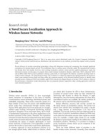
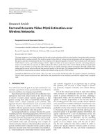
Figure 1: Localized nodes A and B are drawn darker than the unlo-
calized ones, α and β.Ontheleft-handside,α and β are positioned
based only on information about their localized neighbors. As a
result, they are positioned right in the middle, respectively. With
the additional information that α and β are within a mutual radio
range, the area of uncertainty (shown only for α on the right side of
the figure) can be decreased significantly.
(iv) The positioning suggested aims at providing 2D co-
ordinates only. But note that the convex combination
used here works in the same way in 3D, in particular as
we use dimensionless expressions only.
Determining the distance measure itself is not the focus
of this work, but we did some evaluations with the ESB sen-
sor nodes (described in Section 4.1) on the suitability of ra-
dio and sound beacons for distance measurements.
2. PREVIOUS WORK
2.1. Global positioning
Approaches to the global positioning of a node need at least
some nodes which have already acquired their position in
world-coordinates.
The position-aware units may be a small number of ad-
vanced nodes which can be equipped with positioning sys-
tems to serve a much greater number of simple devices. Af-

ter all nodes have been scattered in their destination area
and once each has obtained its position, the failure of the
advanced nodes would no longer be a problem. Similarly, a
small number of simple nodes can be placed manually into
the field of sensors. A human operator would have to obtain
the exact global position, which could then be entered into
the node before dropping it. Despite the simplicity of the ap-
proach, these manually initialized nodes could provide a lo-
cation service for their fellows. The approach trades costs of
nodes against effort for user interaction.
In order to obtain a global position for a node, an equally
weighted average of the coordinates of all position-aware
one-hop neighbors can be built according to an approach
proposed by Bulusu et al. [2]. If the neighboring nodes form
the vertices of a convex patch, then their average lies in the
center of gravity of the patch. In a sense, this approach is
in the spirit of the weighted convex combination proposed
in this paper but with the additional difficulty that no mu-
tual distance measures are available among nodes and that
the quality of the radio or sound signal is not considered in
the calculation of the position. We will, however, utilize this
information in Section 3.
Another equally weighted sum of positions was proposed
by Adebutu et al. [3]. The difference to the approach men-
tioned above is that from the beginning, both location-aware
and unaware nodes are considered, as is shown in Figure 1.
Obviously, position-unaware nodes are not helpful in the be-
ginning. Initially, their position will be set to the position of
an arbitrary neighbor or to that of another first guess. In each
iteration, a node with a yet uncertain position builds the av-

erage coordinates of its neighbors, thus gaining certainty of
its location. In the next iteration, its improved position will
contribute to the calculation of the other nodes’ positions,
which will in the end converge against a stable result. The
approach is a bit stronger than the previous one as it consid-
ers both positioned and not yet positioned nodes. Doherty
et al. [4] adopted the same approach, choosing a linear pro-
gramming scheme for the solution. All location-aware nodes
are represented by constant locations, while nodes with un-
certain positions are variable. The linear program has to be
posed such that none of the existing one-hop connectivities
will be violated.
2.2. Relative positioning
Another class of approaches requires no global coordinates.
Nodes can localize themselves only with regard to their
neighbors. In the beginning, local coordinates are computed
only for the cluster of nodes within the same radio range.
Later, those local coordinates are consolidated into an over-
all base for the entire network. The advantage of relative
positioning is that nodes can estimate distances and angles
among one another just as they would if using global coordi-
nates. However, their location and orientation on the world
map is unknown.
ˇ
Capkun et al. [5] have proposed such approach, which
builds a local coordinate system (CS) if only mutual distances
between nodes within the same proximity are known. The
basic idea is that each node considers itself to be the origin of
its own local CS. Without any global reference it has to define
the direction into which its axes point. For the X-axis, this is

done simply by choosing an arbitrary neighbor. By defini-
tion, the axis is declared to point towards that neighboring
node. So far, this is a very abstract definition, because the
neighbor is unlocalized as well.
The definition of the Y -axis is determined almost im-
plicitly in 2D because it stands perpendicular to the X-axis.
However, its direction can be flipped without violating the
orthogonality constraint. Again, an arbitrary neighboring
node is chosen and the direction of the Y-axis is declared to
point towards that node. With the help of mutual distances,
all remaining nodes in the proximity of the origin can now
be localized within the artificial CS.
Thomas Haenselmann et al. 3
1
5
3
4
a
b
2
n
d
2,n
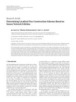
Figure 2: In this example, node n is surrounded by nodes 1, ,5
which form the convex hull of neighbors. a and b are called inner
nodes, which will be ignored at the moment. The location of n has
yet to be determined with the help of the known locations of 1, ,5
and their distances d
k,n
to node n.

This process is repeated by all nodes. The rest of
ˇ
Capkun’s
work deals with consolidating all local CS into a single global
one.
2.3. Triangulation
The process of positioning (here within a plane) by means
of either three known positions and three distances, or two
positions and two angles is referred to in the literature as tri-
angulation.
If three distances are known, circles are drawn around
each of the three anchor points. The radius of each circle cor-
responds to the distance between the anchor point and the
node to be positioned. The circles will yield a common in-
tersection at the position of the floating node. For in-depth
coverage, please refer to [6].
3. PRECISION-AWARE CONVEX COMBINATION
3.1. Introduction to the weighting scheme
We will now address our precision-aware position calcula-
tion, which assumes the following conditions. We consider
an unlocalized node n somewhere in an outdoor space that
has a set of localized neighbors k
∈ 1, , K.Anodek is con-
sidered to be a neighbor of n if both are within the same ra-
dio range and k knows its own global position. Furthermore,
we assume that all neighboring nodes enclose a convex patch
around n. Figure 2 shows an example of such a setting. The
convex patch will be denoted as the neighborhood patch.The
aim of our approach is to derive the location p
n

of the new
node n from the (surrounding) neighbors.
Hint
In case n is not contained in a neighborhood patch, the pro-
posed convex combination is not possible. This can happen
if the node is part of the convex hull of the entire network,
as is true, for example, for node 2 in Figure 2, and there is
another case in which a convex combination will not be pos-
sible. In a very sparsely scattered network, inner nodes may
be connected in one direction only. This would theoretically
be the case if node b was connected to nodes “1,” “2,” and
“a” only. Note that this does not mean that the node in ques-
tion cannot be positioned by triangulation if it has at least
three neighbors. It only means that in these special cases, the
proposed convex combination cannot be applied.
Except for the special case mentioned above, two neigh-
boring nodes on the convex hull i, j
∈{1, , K}in different
places will suffice to localize node n if the distance between i
and n,denotedasd
i,n
, and the distance d
j,n
is known. As de-
scribed in Section 2.3, the two circles around i and j are cho-
sen such that they intersect at node n. They will then produce
two intersections. For the following reason, in our case, only
two nodes suffice to determine a node’s position. In the pro-
posed convex combination, only neighboring nodes on the
convex hull are involved in estimating the position of node n.

As a consequence, one intersection (the valid one) will be in-
side the patch, while the invalid one lies outside. Thus, it can
be excluded in the first place. Another simple way to identify
the right choice for the position of n is to look for a cluster
of suggested positions. Only those positions near the cluster
center are valid in our context; the alternative positions are
scattered around the patch and are not considered. The clus-
ter will be obtained anyway in the subsequent calculation.
3.2. What is the gain of unequal weighting?
As stated above, only two known locations p
i
and p
j
along
with the distances to nodes n, d
i,n
,andd
j,n
are needed to de-
rive the location of node n.However,wehavetokeepinmind
that all distance measures will be more or less disturbed. Ob-
viously, more accurate results can be expected by incorpo-
rating all neighbors rather than relying only on two of them.
We can imagine a situation in which all nodes “provide a
suggestion” for the estimated location p
n
of node n.Some
suggestions by nodes within a close proximity will be more
accurate, while others will be less reliable due to long dis-
tances. So ideally, the position estimate from a near-by node

should contribute more to the calculation of p
n
than the po-
sition suggested by those nodes with weak incoming signals
(the perception of the signal strength is always based on the
perspective of node n).
Our approach expresses the location p
n
by means of a
convex combination [7, 8] of the position suggestions p
(k)
n
coming from each neighbor k, as shown in (2). We denote
the suggestion of node k as (k) in the superscript. The n in
the subscript represents the suggested position of node n
p
n
=
K

k=1
l
k
p
(k)
n
,
K

k=1

l
k
= 1.
(1)
The weights l
k
that define the influence of each position
p
(k)
n
should satisfy the following constraint. As node n ap-
proaches an arbitrary node k, there should be an increasing
contribution of location p
(k)
n
to p
n
. Generally, the contribu-
tion of the location p
(k)
n
to p
n
should be inversely propor-
tional to the distance between n and k, causing nearby nodes
to have more influence on each other than distant nodes will
4 EURASIP Journal on Advances in Signal Processing
1
5
3

4
α
1
α
5
α
4
2
n
α
2
α
3
π
3
= α
1
α
5
α
4
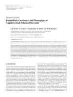
Figure 3: An area α
k
is formed by the inner node n and two neigh-
boring outer nodes of the convex polygon. The product π
3
can be
thought of as the weighting factor of node 3. Note that π
3
consists of

the dark-shaded areas which do not share the common edge between
node n and node 3.
have. Intuitively speaking, we might say that if k is close to n it
will have a better understanding of position of n and should
thus be given a greater weight.
Before going into detail on how to obtain the weights for
each node, we will introduce the atoms from which they are
constructed, namely the areas α
k
. Figure 3 shows that each
area α
k
is formed by the triangle Δ(p
n
p
k
, p
(k mod K)+1
). The
slightly clumsy expression in the subscript (k mod K)+1of
the last vertex of the triangle is required to calculate the area
of α
K
.Forα
K
, the positions of both the last and of the first
nodes are needed, which are obtained by using the mod-
ulo operator. The calculation or area α
k
is done according

to Heron’s formula [9]:
s
= d
k,k+1
+ d
n,k
+ d
n,k+1
,
α
k
=

s

s − 2d
k,k+1

s − 2d
n,k

s − 2d
n,k+1

4
.
(2)
Since the location p
n
is not yet known, the areas α

k
have
to be obtained using the distances between the nodes. This is
done in (2) by means of the distances d
i,j
between two nodes
i and j:
π
k
=

K
i=1
α
i
α
k−1
α
k
= α
1
α
2
···α
k−2
α
k+1
···α
K
.

(3)
Equation (4) almost immediately derives the weights for
each sensor node (or more precisely for the location sug-
gested by each of them) from the weight π
k
in (4). The only
difference between the weights π
k
and the actual weights l
k
that are used for the convex combination in (2)(andwhich
so far have been omitted for didactic reasons) is that the l
k
will be normalized in order to sum up to 1, which is not the
case for the sum over all π
k
.
The calculation of π
k
is now described more intuitively.
To obtain the (unnormalized) weight π
k
, multiply all areas
except for the two areas which share the common edge be-
tween node n and k. Figure 3 makes clear that the two trian-
gles α
2
and α
3
are not included in the product. Now it be-

comes obvious why the influence of a particular node k in-
creasesasitisapproachedbyn. The reason is that, as shown
in Figure 4, the two white areas α
2
and α
3
become smaller
and smaller, while the other three dark areas tend to cover
more of the entire polygon. However, the weight π
3
does not
include the shrinking areas but only the dark-shaded grow-
ing areas. All the other weights π
k=3
actually do include the
shrinking areas in their product. Note that all weights π
k=3
except for π
3
containawhitearea(resp.,asmallfactor)in
their product. Multiplying by a small factor α also renders
the according weights π
k=3
small, while π
3
is not influenced
by the two shrinking triangles.
Finally, (4) defines the actual weights l
k
for the convex

combination in (2), which eventually leads to an optimized
approximation of the true location of n.Thel
k
are simply a
version of the π
k
normalized in order to sum up to 1:
l
k
=
π
k

K
i=0
π
i
. (4)
We did not yet define how to obtain what we have so far
called node k’s “suggestion” p
(k)
n
for the location of node n.At
this point, the reader should not be misled into believing that
a convex combination of the actual locations of the neighbor-
ing nodes may lead to the true location of n as shown in (5):
p
n
=
K


k=1
l
k
p
k
+error

p
n

. (5)
In fact, a simple convex combination of the known world
coordinates p
k
of the neighboring nodes would also result
in an approximation of the location p
n
. Figure 5 displays the
magnitude of the displacement error that would be made us-
ing this particular kind of simplified approximation. Areas
near the vertices of the polygon suffer more than those in the
middle from smaller deviations from the actual coordinates.
It can be shown that the error made using (5) is zero over the
whole polygon only in the special case of equilateral neigh-
borhood polygons.
Obviously, the combination of the neighbors’ coordi-
nates p
k
has to be replaced by using what was already men-

tioned as “node k’s suggestion” p
(k)
n
of the assumed location
p
n
, which is again used in (6):
p
n
=
K

k=1
l
k
p
(k)
n
. (6)
Geometrically, p
(k)
n
is obtained by drawing a circle around
node k, as sketched in Figure 6. Only locations at the bound-
ary of the circle are candidates for location p
(k)
n
. Intersecting
with another circle around node k
−1ork +1providesafirst

estimate. However, there is no need to choose either k
−1or
k + 1 because both of them can be utilized at the same time.
As a result, two valid intersections s
1
and s
2
evolve. The mid-
point p
(k)
n
on the line between both intersections can be used
as an improved approximation of the location of n. Note that
the distance d
k,n
between a node k and a node n can only be
estimated and is thus error-prone. We denote the approxima-
tion of d as

d.Iftheestimateswerecorrect,s
1
and s
2
would
Thomas Haenselmann et al. 5
1
5
3
4
α

1
α
5
α
4
2
n
α
2
α
3
π
3
= α
1
α
5
α
4
Figure 4: As node n approaches node 3, the dark areas α
1
, α
5
,and
α
4
gain area at the expense of the white areas α
2
and α
3

. Since π
3
is composed only of the dark areas, its overall influence converges
against that of the entire polygon area.
No error
Maximum error
Figure 5: Simply combining the known global location of the
neighboring nodes to estimate the coordinates of node n results in
an error of varying magnitude depending on the true location of n.
meet exactly at p
n
, so that two intersections would not be
necessary.
We will show in the next section that this weighted
combination causes a smaller average mistake than does an
equally weighted sum of all p
(k)
n
.
4. EVALUATION OF THE PRECISION-GAIN
Let us quickly summarize what we did in the last section and
analyze the benefits of our approach. A sensor node in an un-
known place has to derive its position with the help of sur-
rounding nodes which already know their global coordinates.
Each of them can estimate the distance to the unlocalized in-
ner node with a degree of uncertainty. By means of triangu-
lation, a first guess of a position can be made with the help of
two nodes.
In a straightforward procedure, the estimates of sur-
rounding pairs of nodes could be averaged. If we interpret

a single position guess as a random variable with a specific
standard deviation σ, then the average out of n samples will
decrease σ by the factor of
√
n.
k −1
k

d
n,k

d
n,k−1

d
n,k+1
k +1
n
p
(k)
n
s
1
n
s
2
Figure 6: Location of node np
(k)
n
is calculated from the viewpoint

of node k. A circle around k is intersected by circles around k
− 1
and k + 1. The two arising valid intersections are denoted as s
1
and
s
2
. The location right between those two intersections can be used
as the approximation p
(k)
n
for the location of n proposed by node k.
In contrast to the equally weighted average, the unequal
weighting scheme aims to improve the precision further by
moving the weights to those nodes which are able to make a
better guess. In more statistical terms, we focus on the con-
tributing nodes with a lower variance while still maintain-
ing the benefits of the mean calculation consisting of several
measures. We exploit the fact that an estimate for a distance
to a distant node tends to be coarser than the guess of a node
in a close proximity.
In this section, we want to analyze under which condi-
tions the unequal weighting scheme improves the precision
gain the most by means of a simulation. Before we go into
detail, we examine in the following subsection under which
circumstances our assumption holds true that estimates of
long distances are coarser as compared to short distances.
4.1. Background on distance estimates
Most positioning approaches need estimates of distances be-
tween nodes. Depending on the capabilities of the hardware,

distances can be derived from the strength of the incom-
ing radio signal, which is often referred to as Received sig-
nal strength indicator (RSSI), for example, in the context of
the RADAR system [10]. As an alternative, the time of arrival
(TOA) or time difference of arrival (TDOA) of beacons be-
tween communicating nodes can be used to estimate mutual
distances.
In order to evaluate the fitness of a typical sensor node
platform, we did some tests on TDOA with radio beacons on
the ESB nodes. However, TDOA did not prove to be a feasible
approach in this context. The main reason is the coarseness of
the internal clock. The Texas Instruments MSP430 processor
used for the ESB nodes is clocked at about 8 MHz. Even if an
incoming bit (which is the shortest unit the transceiver can
send) could be detected within a single cycle of the proces-
sor, it would take 1.25
× 10
−7
seconds. If the signal travels at
about 300 000 km/s, a radio beacon will bridge a distance of
about 37.5 meters within one clock cycle. In practice, the de-
tection of a bit takes much longer on most sensor node plat-
forms since they are not optimized for the fast detection of
radio signals. The order of magnitude of the error and the er-
ror variance introduced by these delays renders TDOA-based
6 EURASIP Journal on Advances in Signal Processing
approaches unsuitable for most of today’s sensor node plat-
forms.
Theoretically,soundbeaconsaremoresuitablefor
TDOA-based positioning on sensor nodes as sound travels

only about 300 m/s. Early work on range estimation using
acoustic sensing has been done by Girod and Estrin using
standard PCs and Linux [11]. Sallai et al. report an average
error of below 10 cm using MICA nodes [12].
On the ESB nodes, a single clock cycle allows sound to
travel only about 0.0375 mm. So even if the detection of the
beacon takes 1000 cycles or more, the accuracy is still suf-
ficient. In our evaluations, the detection of the specific fre-
quency the piezo-buzzer could produce proved to be chal-
lenging. Particularly for longer distances, the microphone
was not sensitive enough to ensure a reliable detection. Fur-
thermore, the 2048 bytes of RAM do not encourage the im-
plementation of sophisticated signal analysis algorithms, es-
pecially since the memory is shared with the operating sys-
tem.
Acoustic distance measurements have also been done by
Sallai et al. [12]. The authors encountered a tight correla-
tion between the sound propagation delay and internode dis-
tances, however, with larger outliers for increased distances.
According to their analysis, these outliers are due, for ex-
ample, to reflections or multipath propagation. These phe-
nomena tend to become more important with increasing dis-
tance, while short distances often allow the signal propaga-
tion along the direct line of sight. So even for TDOA-based
approaches, we can conclude that longer distances tend to
introduce larger errors.
As a consequence of the simplicity of our hardware used,
we tried to focus on the received signal strength. Its simplicity
makes it suitable for very simple devices with no audio sen-
sors and actuators, and even for very constrained resources

of even simpler hardware often referred to as smart dust. The
readings of the signal strength allow only for very coarse dis-
tance estimates, which was the main motivation to come up
with our approach.
As we assume that the hardware has to be used as pro-
vided by the sensor node, we focused on its particular charac-
teristic to find a way to improve the precision of the distance
estimate. It proved to be helpful to have a closer look at the
received radio signal strength s between two nodes, which is
known to degrade inversely proportional to the squared in-
ternode distance d:
s
∼
1
d
2
. (7)
A sensor node samples the incoming signal in equally
sized quantization steps. This means that the resolution of
the received radio signal in the proximity of a node is rela-
tively high. The greater the distance between two nodes, the
larger the interval that has to be covered by a single digital
value. Another more practical cause of error influence is that
the detection of bits, for example, by means of a rising and
falling radio signal, becomes more error-prone over larger
distances on average.
For the sake of completeness we want to mention another
class of positioning algorithms which do not require distance
FLOAT improvement(position P, nodes[k] N)
// calculate distances to all spanning nodes

FOR EACH of the k nodes N[i] spanning the patch
BEGIN
dist
PN[i] = distance(P, N[i])
dist
PN[i] += error(dist PN[i]) // and distrb
by certain error
END
// each triple (i, i + 1, i + 2) of nodes
// creates a position estimate
FOR EACH of the k nodes N[i] spanning the patch
position
suggestion[i] =
triangulate(dist PN[i], dist PN[(i+1)MODk],
dist
PN[(i+2)MODk]
// the final position is a weighted sum
// of the position estimates
estimation
weighted = estimation trivial = 0
FOR EACH of the k nodes N[i] spanning the patch
BEGIN
estimation
weighted += position suggestion[i]
∗ weight[i]
estimation
trivial += position suggestion[i]/k
END
improvement
= ABS(P-estimationtrivial) − ABS(P-

estimation
weighted)
return improvement
Algorithm 1
estimates. They operate based only on the mere connectivity
between nodes. APIT is an instance of these range-free lo-
calization schemes which has been proposed by He et al. It
operates based on beacons that allow a node to determine
whether it is inside or outside a particular triangle [13]. By
intersecting several triangles, the valid area can be narrowed
down successively. Doherty et al. have proposed a convex po-
sition estimation which is also based on simple connectivity
constraints [14]. The authors analyze the precision of posi-
tion estimates in a more or less populated neighborhood. To
take the remaining uncertainty of the estimates into account,
they define bounding boxes for candidate regions.
Niculescu and Nath suggested to use the angle of arrival
(AOA) of a signal to determine the position by means of tri-
angulation. Here, the problem of determining mutual dis-
tances is shifted to determining the direction of a sender [7].
4.2. Assessment of the unequal weighting scheme
Inordertosimulateothertopologiesofnodesorerrorchar-
acteristics than the ones proposed below, our simulator can
be obtained free of charge. (The tar-archive of the simulation
can be obtained at -mannheim
.de/
∼haensel/sensor location.tgz.).
Thomas Haenselmann et al. 7
Table 1: The column example topology shows four example topologies in which the positioned nodes span a patch. Column normal average
shows the mean deviation between the true position and the calculated one for the average computation in absolute distance units. Un-

equal weights column depicts the same calculations based on unequal weights. The mean improvement over the equally weighted average is
provided by column gain.
Example topology Normal average Unequal weights Gain Example topology Normal average Unequal weights Gain
Triangle 27.4 18.7 31.8% Quadrangle 25.3 19.0 24.9%
5 vertices 24.8 19.5 21.4% Colinear 26.2 23.2 11.5%
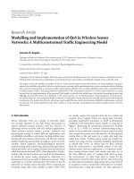
Figure 7: The precision gain of the unequal weighting scheme over
the normal average is displayed for an example topology spanned
by six positioned nodes. The strongest improvements displayed in
dark shades take place at the edges and vertices of the patch. The
improvements vanish towards the center of gravity in the middle
because here the weights become more and more equal, thus con-
verging against an equally weighted average.
In the simulation, the neighborhood patch is built up by
means of the spanning nodes. Then, the software iterates over
each inner position P on a fine-grained grid. For a given posi-
tion P, the pseudo code below evaluates the gain between our
proposed unequal weighting scheme and an equally weighted
one. In particular, the variable estimation
weighted
contains
the error caused by the unequal weighting scheme, while
estimation
trivial
contains the error of the equally weighted av-
erage. Both error values state the spatial distance between the
actual position P and the calculated one. A difference of zero
means that the exact position was calculated. Any other pos-
itive value reflects the magnitude of the distance vector be-
tween P and the assumed position.
In the end, the proposed approach is an improvement

only if its calculated position is closer to the real position P as
compared to the equally weighted scheme. Figure 7 shows a
plot of the positioning improvement return by Algorithm 1.
If the distances dist
P,N
were all precise, the calculated co-
ordinate of P should match the true one, perfectly. However,
in a real-world scenario, those distances can only be guessed
at,aswehavepointedoutinSection 4.1. Depending on the
internode distance, each distance measurement is disturbed
by a certain error in the simulation.
The degree of distortion of a measurement and the im-
provements achieved in the end are put as a fraction of the
radio range below.
The error (error(dist) in the pseudocode) added to the
internode distances never drops below 5% of the radio range
for short distances, and rises to up to 20% for distances up
to the maximum radio range. As stated in Section 4.1, the
assumption is that longer distances are more prone to exhibit
larger errors than are shorter ones.
Figure 7 shows a plot of the improvement over a sample
patch in which darker areas indicate stronger improvements
and lighter areas less improvement. Obviously, the vertices
and the boundary of the patch profit more from the unequal
weighting scheme, while the inner part of the patch exhibits
no significant gain. The reason for this is that the positions
in the middle are about equally distant from the spanning
nodes. As a consequence, their weights are also more or less
equal. So the positioning quality between the equally and un-
equally weighted scheme can only be marginal, the more a

position P converges into the center of gravity of the patch.
Ta bl e 1 and the accompanying Figure 8 provide a closer
quantitative analysis of the precision gain over the different
patch topologies.
Figure 8 shows different configurations of nodes, a tri-
angle, a rectangular quadrangle, and an irregular shape with
five vertices. Again, the darker shades show regions in which
larger improvements can be achieved, while the light shades
depict areas with little or no improvement. All images includ-
ing Figure 7 exhibit a noisy salt-and-pepper-like structure, in
particular in the darker areas. This shows that positioning
improvements occur irregularly. In other words, some posi-
tions profit highly from the unequal weighting, while others
are hardly or not at all influenced.
Responsible for this phenomenon is the introduced error.
As described above, the inter-node distances are disturbed
as much as 20% of the node’s radio range. However, the
equally distributed random error can by coincidence cause
both strong disturbances or none at all. So sometimes the
distortion of the inter-node distances will by chance be close
to zero. If the error is small or negligible, then the differ-
ence between the results of the equal and the unequal weight-
ing schemes can also only be marginal. Because all the sum-
mands of which the weighted average consists are good es-
timates. And moving the weight from one good estimate to
another hardly alters the final result. As a consequence, the
precision gain will be negligible as well.
For a more intuitive example, the reader may imagine
the bullet holes caused by a shotgun. Some will be strong
outliers, while others may be clustered close to the target

point. Calculating the target point based on those which are
closely scattered around the actual target will result in a good
approximation, which is what the weighted average tries to
achieve. However, including all outliers with a high variance
will result in a higher variance of the average as well, thus
yielding worse results. However, if by chance there are no
8 EURASIP Journal on Advances in Signal Processing
Positioning error
improved on avg.:
Region 1: 5%
Region 2: 20%
Region 3: 30%
Region 4: 40%
Region 5: 50%
4
3
2
1
(a) Three nodes span a triangular patch
5
4
3
2
1
(b) Rectangular quadrangle
5
4
3
2
1

(c) Five vertices of which four
nodes form two pairs
5
4
3
2
1
(d) Four almost colinearly positioned
nodes spanning a slim patch
Figure 8: Different topologies of nodes were evaluated to assess their positioning gain. Numerical figures are given in Ta bl e 1 . Obviously,
the largest improvements which cut down the error about 50% on average are made at positions which have neighbors (the vertices of the
polygon) near by and in a larger distance. Unequal positioning achieves the least improvements if all nodes have about the same distance (in
the middle of the polygons).
strong outliers, weighting some bullet holes unequally will
not change the average position significantly.
Ta bl e 1 shows the positioning gain. For the triangle, we
can see that the deviation of the distance in absolute units is
27.4 for the equally weighted sum and 18.7 for the unequally
weighted sum. This means that on average, an improvement
of about 31.8% was achieved. For the other topologies, the
error can be cut by 25%–21% which is a significant improve-
ment, given that the scheme exploits the characteristics of the
measurements only and does not alter the hardware at all.
Figure 8(d) shows another topology of four nodes that
are almost co-linear. As a result, they form a long and narrow
patch. In this simulation, the gain the unequal positioning
can achieve is lower, at only about 11%. This effect can be
explained by the patch’s geometry. As seen in the examples of
Figure 8, the outer regions of the patch profit most from the
proposed scheme.

Let us consider a circular patch. If we increase the ra-
dius, the outer area increases proportional to the square of
the radius. In contrast, a linear structure increases propor-
tional only to its length. Though the slim patch has an area
as well, it’s growth does not result in a significant gain in the
beginning.
Put into more mathematical terms: the function f (x)
=
x
2
remains close to the abscissa for some time before gaining
large values. For this reason, mostly colinear structures gain
area only after significant scaling. So the outer parts of these
patches which profit most from the proposed approach do
not grow that easily, which results in smaller improvements
since the ratio between the outer regions which profit much
and the inner regions which profit least remains more equili-
brate for some time. Even more formally we can simply state
that x
×x grows faster than (x + c) ×(x −c).
The degenerated patch of Figure 8(d) does not play an
important role in practice since a set of randomly scattered
nodes do not often produce these topologies.
4.3. Computational requirements
In the context of sensor networks, the feasibility and the effi-
ciency of an algorithm have to be taken into account. The cal-
culations we performed are composed of a sum of estimates
p
(k)
n

with one weight l
k
for each summand (see (6)). Since
the weights l
k
essentially are the triangular areas π
k
, scaled
in order to sum up to one, the total effort is increased only
by a constant factor. Only the areas π
k
are each composed
of all distance estimates. So n neighbors lead to a compu-
tational effort proportional to O(n
2
). A number of about 10
neighbors lead to several hundred multiplications, additions,
and a few root calculations. However, even the highly energy
efficient MSP430 processor running at 8 MHz can perform
about 2.6 million instructions per second with an average
number of three clock cycles per instruction. Since the ar-
chitecture has zero wait states (the memory is in sync with
the processor), this performance is actually achieved. After
all, the calculations only have to be done once in the startup
phase of the network, so the requirement for additional time
and energy is negligible.
5. CONCLUSION AND OUTLOOK
We have proposed an approach to positioning a wireless
sensor node by means of the distance from surrounding
nodes with known world coordinates. We consider each lo-

calized node to suggest a new node’s position. But not all
suggestions will be of the same quality. The distant nodes
Thomas Haenselmann et al. 9
will propose coordinates with greater uncertainty than will
nearby nodes. The position of the unlocalized node is ob-
tained by a weighting scheme which emphasizes coordinate
suggestions of nearer nodes, thus gaining certainty over the
new node’s true position.
From the field tests with the ESB platform, we know that
the degradation of signal quality is not influenced signifi-
cantly by the internode distances up to a certain range, but
drops relatively fast at a further distance. In our future work
we will try to adapt the weighting scheme more closely to the
reception characteristics in order to strengthen the influence
of nodes within the more deterministic shorter rang.
APPENDIX
Our evaluation is based on a simulation, which we pro-
vide for download under the GPL at www.informatik.uni-
mannheim.de/
∼haensel/location simulation.tgz.
It runs under GNU/Linux using the simple direct media
layer (SDL). The polygon can be chosen arbitrarily but has to
be defined in the source code in the beginning.
REFERENCES
[1] U. E. Ruttimann, R. A. J. Groenhuis, and R. L. Webber,
“Restoration of digital multiplane tomosynthesis by a con-
strained iteration method,” IEEE Transactions on Medical
Imaging, vol. 3, no. 3, pp. 141–148, 1984.
[2] N. Bulusu, J. Heidemann, and D. Estrin, “GPS-less low-cost
outdoor localization for very small devices,” IEEE Personal

Communications, vol. 7, no. 5, pp. 28–34, 2000.
[3] T.Adebutu,L.Sacks,andI.Marshall,“Simplepositionestima-
tionforwirelesssensornetworks,”inLondon Communications
Symposium (LCS ’03), pp. 300–305, London, UK, September
2003.
[4] L. Doherty, K. S. J. Pister, and L. El Ghaoui, “Convex position
estimation in wireless sensor networks,” in Proceedings of the
20th Annual Joint Conference of the IEEE Computer and Com-
munications Societies (INFO COM ’01), vol. 3, pp. 1655–1663,
Anchorage, Alaska, USA,, April 2001.
[5] S. Capkun, M. Hamdi, and J. Hubaux, “GPS-free positioning
in mobile ad-hoc networks,” in Proceedings of the 34th Hawaii
International Conference on System Sciences (HICSS ’01),p.
255, Big Island, Hawaii, USA, January 2001.
[6] T. Haenselmann, An FDL’ed Textbook on Sensor Networks,
chapter 3, 4, University of Mannheim, Mannheim, Germany,
2007.
[7] D. Niculescu and B. Nath, “Ad hoc positioning system (APS)
using AOA,” in Proceedings of the 22nd Annual Joint Conference
of the IEEE Computer and Communications Societies (INFO-
COM ’03), pp. 1734–1743, San Francisco, Calif, USA, March-
April 2003.
[8] C. T. Loop and T. D. DeRose, “Multisided generalization of
Bezier surfaces,” ACM Transactions on Graphics,vol.8,no.3,
pp. 204–234, 1989.
[9] D. P. Robbins, “Areas of polygons inscribed in a circle,” The
American Mathematical Monthly, vol. 102, no. 6, pp. 523–530,
1995.
[10] D. Niculescu and B. Nath, “Dv based positioning in ad hoc
networks,” Telecommunication Syste ms,vol.22,no.1—4,pp.

267–280, 2003.
[11] L. Girod and D. Estrin, “Robust range estimation using acous-
tic and multimodal sensing,” in Proceedings of IEEE Interna-
tional Conference on Intelligent Robots and Systems (IROS ’01),
vol. 3, pp. 1312–1320, Maui, Hawaii, USA, October 2001.
[12] J. Sallai, G. Balogh, M. Mar
´
oti, A. L
´
edeczi, and N. Kusy,
“Acoustic ranging in resource constrained sensor networks,”
Tech. Rep. ISIS-04-504, Institute for Software Integrated Sys-
tems, Vanderbilt University, Nashville, Tenn, USA, 2004.
[13] T. He, C. Huang, T. Abdelzaher, B. M. Blum, and J. A.
Stankovic, “Range-free localization schemes for large scale
sensor networks,” in Proceedings of the 9th Annual Interna-
tional Conference on Mobile Computing and Networking (MO-
BICOM ’03), pp. 81–95, San Diego, Calif, USA, September
2003.
[14] L. Doherty, K. S. J. Pister, and L. El Ghaoui, “Convex position
estimation in wireless sensor networks,” in Proceedings of the
20th Annual Joint Conference of the IEEE Computer and Com-
munications Societies (INFO COM ’01), vol. 3, pp. 1655–1663,
Anchorage, Alaska, USA,, April 2001.