Báo cáo hóa học: " Research Article Determining Localized Tree Construction Schemes Based on Sensor Network Lifetime" doc

Hindawi Publishing Corporation
EURASIP Journal on Wireless Communications and Networking
Volume 2010, Article ID 350198, 13 pages
doi:10.1155/2010/350198

Research Article
Determining Localized Tree Construction Schemes Based on
Sensor Network Lifetime
Jae-Joon Lee,1 Bhaskar Krishnamachari,2 and C.-C. Jay Kuo2
1 Jangwee

Research Institute for National Defence, Ajou University, Suwon 443-749, Republic of Korea
of Electrical Engineering, University of Southern California, Los Angeles 90089-2564, CA, USA

2 Department

Correspondence should be addressed to Jae-Joon Lee,
Received 27 October 2009; Revised 2 June 2010; Accepted 1 July 2010
Academic Editor: Yu Wang
Copyright © 2010 Jae-Joon Lee et al. This is an open access article distributed under the Creative Commons Attribution License,
which permits unrestricted use, distribution, and reproduction in any medium, provided the original work is properly cited.
The communication energy consumption in a data-gathering tree depends on the number of descendants to the node of concern
as well as the link quality between communicating nodes. In this paper, we examine the network lifetime of several localized tree
construction schemes by incorporating the communication overhead due to imperfect link quality. Our study is conducted based
on empirical data obtained from a real-world deployment, which is further supported by mathematical analysis. For the case of a
sparse node density, a large network size and a low link threshold, we show that the link-quality-based scheme provides the longer
network lifetime than the minimum hop routing schemes. We present a lower bound on the number of nodes per hop and the
link quality threshold of the radio range, which work together to result in a superior localized scheme for longer network lifetime.

1. Introduction
For data-gathering path construction, nodes have to determine the next node to forward the data to the sink with

a parent selection strategy. A localized tree construction
scheme allows each node to select a parent node using its
one-hop neighboring node information. Thus, the purpose
of localized schemes is to reduce the communication overhead for the construction of a data-gathering path, which
is desirable for energy-constrained wireless networks. Even
though there have been studies on wireless network lifetime
[1–6], and a few studies on localized tree construction
[7], the effect of localized tree construction scheme on
the network lifetime has not been extensively examined.
Here, we examine localized tree construction schemes with
different parent selection strategies and analyze their impact
on the network lifetime in conjunction with diverse network
conditions such as node density, network size, and link
quality between communicating nodes.
The routing path selection in conjunction with link
quality have been examined in several studies. De Couto
et al. present a path selection metric, which is called
expected transmission (ETX) count. This metric is used to
select the minimum number of transmissions required for

successful delivery to a destination among different paths
by incorporating the quality of each link on the path in
[8]. Draves et al. provide comparison among path selection
schemes based on link quality metrics and minimum hop
counts through detailed experiment in [9]. They find that
the expected transmission (ETX) count scheme provides
higher throughput than minimum hop count scheme when
a DSR routing protocol [10] is used with stationary nodes.
Woo et al. [11] examine the effect of link quality on
different routing strategies in terms of hop distribution, path

reliability, success rate from a source to the sink, and path
stability. In their work, the minimum expected transmission
scheme results in the highest end-to-end success rate. Seada
et al. [12] present the analysis of forwarding strategies by
incorporating link quality and calculate the energy efficiency
in geographic routing. They show that the product of a
packet reception rate and a distance metric provides the most
energy efficient geographic forwarding path. In addition to
the above work, several studies including [13, 14] examine
the link quality effect on connectivity.
In this paper, we examine several localized tree construction schemes and point out the trade-off between linkquality-based schemes and minimum-hop-routing-based
schemes in terms of network lifetime. If we use high quality


2

EURASIP Journal on Wireless Communications and Networking

links to reduce the number of retransmissions, the number
of descendants to be processed in the data-gathering tree will
increase, which results in the increase of energy consumption
for communication due to more data. On the other hand, if
we decrease the amount of forwarded data by distributing
workload to more nodes, selected link’s quality may not
be the best and retransmissions can increase. Our study
is conducted as follows. First, we examine the empirical
data obtained from a real-world sensor deployment to
capture the effects of different tree construction schemes on
energy consumption. Then, to obtain the insight into the
above trade-off and derive criteria to reach longer network

lifetime, the energy consumption of each scheme is analyzed
and compared. Finally, the global optimum is presented
and compared with the analytical results of different tree
construction schemes.
Our study shows that when the network size is small
and the node density is high with a high link threshold
(i.e., minimum packet reception rate that determines onehop direct link or not between two nodes), minimum hop
routing schemes achieve longer network lifetime than the
scheme whose selection is based only on the link quality.
However, with the opposite network conditions, the linkquality-based scheme can achieve longer network lifetime.
We present lower bound on the number of nodes in a hop
as a function network size, transmission energy portion,
and radio range link quality, which guarantees that the
load-balanced scheme achieves longer lifetime than the linkquality-based scheme. In addition, we present lower bound
on link threshold as a function of node density, which
guarantees the longer lifetime of the load-balanced scheme
regardless of other network conditions such as the network
size and the transmission energy portion. When the link
√
threshold is less than 1/ 2, the load-balanced scheme does
not guarantee longer lifetime than the link-quality-based
scheme in 1D linear topology and 2D grid topology.
The localized data-gathering tree construction schemes
with different parent selection criteria are described in
Section 2. We examine the effect of these schemes on energy
consumption and network lifetime by incorporating a link
quality metric and the communication load distribution
based on the empirical data in Section 3 as well as analysis
in Section 4. Criteria for superiority of a localized scheme
in terms of network lifetime are analyzed in Section 5. The

comparison with the global optimal strategy is presented in
Section 6. Finally, concluding remarks and future research
directions are presented in Section 7.

2. Localized Tree Construction Schemes
Data-gathering path can be selected based on the diverse
criteria. The link quality can be used as a metric for routing
path selection. Recently, the expected transmission (ETX)
count of a link between two nodes is considered, which can
be derived from the packet reception rate (PRR) of the link
[8, 9]. Mathematically, we have
ETXi j = ETX ji =

1
,
PRRi j · PRR ji

(1)

where ETXi j is the expected number of transmission
required for successful transmission over a link between
nodes i and j. Qualitatively speaking, a low ETX link can
require less energy consumption due to redundant retransmission than a higher ETX link. However, the quantitative
effect of a link-quality-based path selection scheme on energy
consumption and/or network lifetime has not been fully
investigated before.
Besides link quality, the number of hops (called the hop
count) to the destination is widely used for routing path
selection. Each link can be counted as one hop. Then, the
routing path with the minimum number of hop counts to the

sink is the shortest path. The minimum hop routing (MHR)
path can be constructed using the currently known hop
level of neighboring nodes. In order to know its minimum
hop level, the sink node sends the broadcasting message to
all nodes initially once. In the MHR, each node selects a
neighbor node in the upper hop level, which provides the
minimum number of hops to the sink. Detailed discussion
of energy consumption in the MHR can be found in [15].
Rigorously speaking, the link quality and the radio range
will also affect energy consumption in addition to the hop
counts. Here, we incorporate the link quality into the energy
consumption analysis of MHR schemes. By using the ETX
link quality metric and the hop count to the sink, we
will examine the following four localized tree construction
schemes.
(i) The lowest ETX parent selection scheme, where a
node selects a neighbor node that provides the lowest
ETX link between each other and is closer to the sink.
This scheme does not necessarily select a node in the
upper hop level and accordingly the minimum hop
(shortest path) routing may not be achieved.
(i) The random parent selection scheme with the MHR,
where a node randomly chooses a parent among
neighbor nodes in the upper hop level, which provides the minimum hop routing to the sink.
(i) The lowest ETX parent selection scheme with the
MHR, where a node chooses its neighbor node in the
upper hop level that provides the lowest ETX.
(i) The balanced parent selection scheme with the MHR,
where a node selects the neighbor node in the upper
hop level that has the fewest number of children as a

parent in the data-gathering tree.
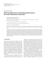
The data-gathering trees for the lowest ETX parent selection
and the minimum hop routing schemes are illustrated in
Figure 1.
The first scheme does not utilize the hop count but the
link quality metric only while the other three schemes take
the hop count into consideration for parent selection as well.
These localized schemes are examined by real empirical data
and analysis in the following sections.

3. Case Study with Real Empirical Data
In this section, with the empirical data in a real deployment,
we examine four localized tree construction schemes to


EURASIP Journal on Wireless Communications and Networking

Sink

Radio
range

(a) The lowest ETX parent selection

3

Sink

Hop = 1 Hop = 2 Hop = 3

Radio
range

(b) The minimum hop routing

Figure 1: The illustration of the data-gathering tree with the lowest ETX parent selection and the minimum hop routing schemes.

understand their impact on the communication load and
discuss their differences. The data are from the experiments
conducted by the UCLA/CENS group [16], where the PRR of
each node from all other nodes is given. A set of 55 nodes was
deployed in the ceiling of the lab in their indoor experiment.
With this PRR information, we examine the connectivity between adjacent hop levels and the communication
overhead distribution among nodes. Without respect to a
target node, any other node that has a PRR for bidirectional
links higher than the link threshold is called its neighboring
node. In other words, every pair of neighboring nodes can
directly communicate with each other if the successful packet
transmission and reception rates are above the link threshold.
Communication to all the other nodes may require multihop
forwarding through neighboring nodes. The link threshold
can be adjusted, which will change the hop level of nodes
from the sink. The use of this threshold makes routing more
reliable. As the link threshold increases, a constructed tree
with more hop levels can provide higher throughput due to
higher successful transmission rate of the link than a simple
minimum hop count routing.
3.1. Data-Gathering Topology Maps. Figure 2 shows the
deployment map of 55 sensor nodes and hop levels with
four different tree construction schemes. A line represents a

data-gathering link between adjacent hop levels, which will
be discussed further. To forward the data to a sink, which is
assumed to be located at Figure 2(a), each node should select
a parent node towards the sink among neighboring nodes to
construct a data-gathering tree. Nodes that have connection
with the sink with the packet transmission and reception
rates higher than the link threshold belong to the first-hop
level and are represented by a diamond shape. For the lowest
ETX parent selection, since the main objective of this scheme
is to provide a high packet successful transmission rate, the
link threshold for the first-hop level is set to 0.95. For all the
other schemes that are based on the minimum hop routing
(MHR), the link threshold is set to 0.9.
As shown in Figure 2(a), the lowest ETX parent selection
without hop count consideration results in longer hop levels.

The longest hop level is 7. Since each node uses the lowest
ETX parent selection, the distance between the parent and
the children nodes tends to be close and the number of hop
levels increases. All possible direct links between adjacent
hop level nodes by the random parent selection scheme with
MHR are presented in Figure 2(b). Each node randomly
selects one among nodes that are connected with a direct link
as its parent node. As the distance from the sink increases,
the first-hop nodes have more direct links to the second-hop
level nodes. With the link threshold 0.9, the MHR scheme
significantly reduces the hop count as compared with the
lowest ETX scheme in Figure 2(a). Figure 2(c) shows the
connectivity graph of the lowest ETX parent selection with
MHR. Since each node selects the lowest ETX neighboring

nodes in the upper hop level, the selected parent nodes tend
to be located at the edge of the hop level, closer to the
second-hop level nodes. For the balanced scheme shown in
Figure 2(d), data forwarding paths to the sink are almost
evenly spread among the first-hop level nodes.
We can summarize observations from these topology
maps produced by four localized schemes as follows. If
we exploit only link quality without using the hop count
in the parent selection decision, the distance between the
chosen link becomes relatively short and hop levels increases
accordingly. When the MHR scheme is used, the linkquality-based selection results in an unbalanced topology
where fewer nodes at the border of hop levels handle most
data forwarding tasks from larger hop level nodes.
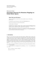
3.2. Link Quality and Communication Load. There exists
trade-off between the link-quality-based and the MHR-based
schemes, which will be examined in this section. Figure 3
shows the average link quality (ETX) of data forwarding
paths selected by four localized tree schemes. The link
threshold varies from 0.7 to 0.9. Regardless of the link
threshold, we observe that the average link quality has the
following order from the highest to the lowest: the lowest
ETX selection, the lowest ETX selection with MHR, the
random selection, and the balanced selection. The reason
for the poor link quality for the balanced selection scheme


4

EURASIP Journal on Wireless Communications and Networking
9

9
Sink

6

Sink

55

8

7

9

16

10

40

31

32

25

22

11

6

13

51

49

54

24

18

2

3

14

8

7

9

16

10

40

31

32

25

22

11

6

13

51

49

54

24

18

2

3

14

39

47

53

23

19

1

5

12

36

6

55

33

7

46

35

8

52

37

46

33

7

52

35

8

50

41

15

27

21

5

5

37

39

47

53

23

19

36

50

41

15

27

21

1

5

12

4

4
3

3

4

4

2

42

38

48

30

28

20

2

42

38

48

30

28

20

1

44

43

45

29

26

17

1

44

43

45

29

26

17

0

0

2

4

6

Hop = 1
Hop = 2
Hop = 3
Hop = 4

8

10

12

0

0

2

6

8

10

12

Hop = 1
Hop = 2
Hop = 3

Hop = 5
Hop = 6
Hop = 7

(b) Random parent selection (MHR)

(a) Lowest ETX parent selection
9

9
Sink

46

55

8

7

9

16

10

35

40

31

32

25

22

11

6

13

6

33

51

49

54

24

18

2

3

14

37

39

47

53

23

19

1

5

12

3

36

50

41

15

27

21

2

42

38

48

30

28

20

1

44

43

45

29

26

17

46

55

8

7

9

16

10

8

40

31

32

25

22

11

6

13

7

33

7

Sink

52

52

35

8

51

49

54

24

18

2

3

14

6
5

5

37

39

47

53

23

19

3

36

50

41

15

27

21

2

42

38

48

30

28

20

1

44

43

45

29

26

17

1

5

12

4

0

4

4

4

4

0

2

4

6

8

10

12

Hop = 1
Hop = 2
Hop = 3
(c) Lowest ETX parent selection (MHR)

0

0

2

4

6

8

10

12

Hop = 1
Hop = 2
Hop = 3
(d) Balanced parent selection (MHR)

Figure 2: The indoor deployment location of nodes and four data-gathering topology maps with localized tree construction schemes using
the PRR data obtained by UCLA/CENS group: (a) the lowest ETX parent selection, (b) the random parent selection scheme (all possible
links) with MHR, (c) the lowest ETX parent selection scheme with MHR, and (d) the balanced parent selection scheme with MHR.

is that it chooses a parent node with the fewest children,
which is consequently far from a selecting node. As the link
threshold increases, the average link quality improves for
both the random selection and the balanced selection scheme
while the lowest ETX selection remains almost the same.
The amount of communication energy of a node during
a data-gathering round is determined by the amount of data
received from children nodes and transmitted to the parent

node and their link quality (ETX). Basically, the amount of
data received from a child node is the product of the link
ETX from that child node and the amount of data that is
transmitted by that child node. As discussed in other work
such as [17, 18], since receiving of corrupted packet incurs
energy consumption at the receiving node, retransmission
of packets increases energy consumption not only at the
transmitting node, but also at the receiving node.


EURASIP Journal on Wireless Communications and Networking

Expected transmission counts (ETX)

1.2

1.15

1.1

1.05

1

0.7

0.75

0.8
0.85
Link threshold

Lowest ETX
Random + MHR

0.9

Lowest ETX + MHR
Balanced + MHR

Figure 3: The comparison of localized tree construction schemes:
the average ETX of data-gathering paths with respect to link
threshold.

Thus, the amount of communication energy per datagathering round by node i can be calculated as
Ei =

f ji ETX ji + β
j ∈Ci

fik ETXik ,
k∈Pi

(2)

where Ei is the normalized energy consumption with respect
to the energy consumption for receiving denoted by Erx and
β=

Eamp
Etx
=1+
,
Erx
Eelec dκ

(3)

where Eamp and Eelec denote the amplifier energy and the
electronic energy, respectively, and d is the radio range and
κ is the path loss exponent similar to [19]. By following
the parameters given in [1], we set Eelec = 50 nJ/bit and
Eamp = 100 pJ/bit/m2 . Besides, when d = 20 m and κ = 2,
β = 1.8. We use Ci to denote the set of children nodes of i and
Pi the set of parent nodes of i. The localized selection scheme
chooses one parent, and f ji consists of data generated by the
descendant nodes of node j in addition to the data generated
by node j. Thus, fik consists of j ∈Ci f ji and data generated
by node i.
When the amount of generated data by each node per

data-gathering round is assumed to be one unit, the number
of descendants in the data-gathering tree constructed by
localized tree schemes determines the communication load
of each node. For the lowest ETX without MHR, there exists
a larger communication load on the first-hop nodes due to
longer hop levels and fewer first-hop nodes. The maximum
number of descendants obtained from Figure 2(a) is 33.
When MHR is used, the communication load is distributed
among a larger number of first-hop nodes than the case of the
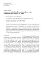
lowest ETX without MHR. Figure 4 compares the number
of children nodes as a function of the distance between the

5

sink and the first-hop level nodes for three different tree
construction schemes with MHR. For the random parent
selection, the expected number of children of first-hop node
p
i is calculated as j ∈Ci 1/n j , where j is a node belonging
to the second-hop level neighboring nodes of node i(Ci ),
p
and n j is the number of upper hop level neighboring nodes
of node j. Since there are only two nodes in the third hop
level, the number of children and descendants are almost
the same.
Overall, the number of descendants tends to increase
along the distance in the random selection scheme. The
lowest ETX parent selection scheme can provide higher
throughput at a given time, but it results in an extremely
unbalanced communication load. This causes much faster

energy depletion of some nodes so as to result in a large gap
of energy depletion time among first-hop level nodes. The
balanced parent selection scheme provides a similar energy
depletion time among nodes.
In this paper, the maximum energy consumption,
denoted by maxi Ei , is defined to be the time before the
death of the first node. The duration in which all nodes are
functional is called the network lifetime. As discussed in [15],
even if workloads are different among the first-hop nodes
due to the use of different parent selection schemes with same
hop levels, the energy depletion time of the last surviving
node in the first hop would be the same. Thus, we focus on
the time before the death of the first node.
Figure 5 compares the maximum energy consumption
of different localized tree construction schemes with the
MHR when the maximum energy consumption of the lowest
ETX without MHR is scaled to 1. The link quality based
schemes result in significantly faster initial energy depletion
while they provide high link quality. The balanced scheme
maintains the initial network operation for longer time and
the random selection scheme has relatively longer network
lifetime, too. However, this observation is obtained from a
small network with few hop levels and nodes. We need more
general discussion to analyze the trade-off among various
localized tree construction schemes with different network
parameters in the following section.

4. Analysis of Localized Tree
Construction Schemes
In the last section, we examined the effect of different

localized tree schemes on communication loads for one real
deployment case. It was observed that the effect of link
quality is not significant when MHR has a relatively large
number of nodes in the first hop, since the communication
load can be distributed and the energy consumption of
a single node is reduced accordingly. However, it is not
clear from this empirical data set whether a lower node
density with a small number of nodes in the first hop
produces the same result. In this section, we characterize
how diverse network conditions (such as the node density
and the network size) affect the energy consumption of each
localized tree construction scheme in conjunction with the
link threshold. Based on the analysis in this section, we
examine whether a balanced scheme can always produce


6

EURASIP Journal on Wireless Communications and Networking
14

12

12

12

10
8
6

4
2
0

Number of nodes

14
Number of nodes

Expected number of nodes

14

10
8
6
4
2

0

2
4
6
8
Distance from the sink

10

Number of descendants

Number of children
(a) Random parent selection

0

10
8
6
4
2

0

2
4
6
8
Distance from the sink

0

10

0

Number of descendants
Number of children

2
4

6
8
Distance from the sink

10

Number of descendants
Number of children

(b) Lowest ETX parent selection

(c) Balanced parent selection

Figure 4: The number of descendants for the first-hop level nodes as a function of their distance to the sink under three parent selection
schemes with MHR.

0.5

PRR = 0.1

Maximum energy consumption ratio

PRR = 0.5
PRR = 0.8

0.4

PRR = 1
Sink

0.3

1

2

3

4

5

···

N −1

N

Figure 6: Illustration of the linear topology.
0.2

0.1

0

0.7

0.75

0.8

0.85
Link threshold

0.9

Random + MHR
Lowest ETX + MHR
Balanced + MHR

Figure 5: The ratio of the maximum energy consumption of MHR
schemes to the maximum energy consumption of the lowest ETX
scheme.

longer network lifetime than the link-quality-based scheme
for any network conditions in the next section.
4.1. Energy Consumption of Localized Schemes. To capture
the effect of tree construction schemes with respect to
the node density and the network size, we examine the
communication load of the linear topology as given in
Figure 6, where nodes are deployed linearly with equidistance. Furthermore, analysis of 2D topology is conducted
in Section 5.2 to derive the criteria needed for a localized
scheme to reach longer network lifetime.
The average link quality (PRR) is a decreasing function of
the distance from the transmitting node as presented in [13].

Following the PRR model in [13], we adopt the approximate
PRR as a function of the distance, whose decreasing rate
accelerates along the distance until the PRR reaches 0.5. The
notation used in this analysis is summarized in Table 1. Note
that, when dr = d1 , there would be only one way to forward

the data to the sink. The only possible parent is the next
node to the sink, which does not require any analysis and
comparison. Thus, we consider the cases where dr is greater
equidistance,
than d1 . In the case of linear topology with √
dr ≥ 2d1 . In the case of 2D grid topology, dr ≥ 2d1 .
Some considerations in our analysis are explained below.
While there could be fluctuation in link quality even in
the static node deployment, energy depletion time can be
analyzed through a long-term average of link quality for
a given link length. In addition, as discussed in previous
work [14, 20], temporal variation of link quality should be
minimal for links with good quality. It is worthwhile to
point out that the PRR is actually the result built upon all
underlying layer interactions. Since our focus is the longterm effect of the routing layer on network lifetime, we use
the PRR to represent the cumulative effect of all underlying
layers (including the MAC layer). Investigation on energy
consumption with MAC layer interactions is an interesting
research topic, which has been studied in previous work, for
example, [21, 22].
4.1.1. Lowest ETX Parent Selection. For the lowest ETX
parent selection scheme as shown in Figure 7, since the link


EURASIP Journal on Wireless Communications and Networking

7

Table 1: Summary of notation.
N

Total number of nodes (network size)
Number of nodes in one hop level with
MHR in linear topology
Number of children of node i
Number of descendants of node i
Energy consumption of node i per round
Distance between the nearest adjacent nodes
Radio range determined by link threshold
Distance between sink and the furthest node
(network radius)
Number of nodes in a radio range
Expected transmission count (ETX)
between nodes i and j, and distance d
Link threshold ETX and PRR

r
nc
i
nd
i
Ei
d1
dr
dN
Nr
ETXi j , ETX(d)
ETX(dr ), PRR(dr )

Sink

1

2

3

4

5

···

N −1

Sink

2 ··· r

1
dr

Hop = 1

N

Hop = 2

Figure 8: The random parent selection scheme with MHR.

the maximum distance from the node that satisfies the link
threshold. To calculate the maximum energy consumption
for the random parent selection scheme with MHR, we first
obtain the expected number of children of each node since
each node selects a parent node randomly with an equal
probability among upper hop level neighboring nodes within
the radio range as shown in Figure 8. Since the expected
number of children attached to node i can be calculated as
p
j ∈Ci 1/n j , the ith node in the first-hop level, with 1 ≤ i ≤ r,
has the expected number of children as

N

i

E nc =
i

to the closet neighboring node provides the lowest ETX, each
node selects its adjacent node that is closer to the sink as the
parent node, that is, the next hop to the sink. Accordingly,
each hop consists of one node and the maximum hop level
is N. Thus, node 1, which is next to the sink, has the largest
communication load to handle data-gathering (arg maxi nd =
i
1). Thus, the energy consumption of node 1 determines the
network lifetime, which is defined to be the initial node death
time.
To analyze the energy consumption, we incorporate the

link quality between adjacent nodes of node 1 in the datagathering tree. When every node generates and sends one
unit of data to the sink, the expected number of data units
received from children of node 1 is ETX(d1 )(N − 1), where
ETX(d1 ) is the number of transmission between nodes that
are one-node apart and d1 is the node distance. The child of
node 1 is its adjacent node; that is, node 2. In addition, the
expected number of transmission from node 1 to the sink is
ETX(d1 )N. Thus, the energy consumption by node 1 during
a data-gathering round, which is normalized in terms of the
reception energy consumption based on the notation in (2)
is equal to
i

···

dr

Figure 7: The lowest ETX parent selection scheme.

max Ei = E1 = ETX(d1 )(N − 1) + βETX(d1 )N,

· · · 2r

r +1

(4)

which is the maximum energy consumption by the lowest
ETX parent selection scheme.
4.1.2. Random Parent Selection with MHR. The link threshold is used to determine the neighboring nodes that can

directly communicate in a single-hop in the MHR schemes.
Thus, each node selects a parent node in the upper hop level
neighboring nodes within the radio range dr , where dr is

1
.
r − j+1
j =1

(5)

The rth node, which is furthest from the sink among the firsthop nodes, has the maximum expected number of children
(arg maxi nc = r) as rj =1 1/ j.
i
The expected number of descendants of node i can be
calculated recursively as
i

1 + E nd j
r+
j =1

1
.
r −i+1

(6)

The largest expected number of transmission from children
to a first-hop node, which is to node r, is

r

max f rxi =
i

ETX d j

1 + E nd j
r+

j =1

1
.
r − j +1

(7)

The expected number of transmission to a sink from node r
is
⎛

max ftxi
i

= ETX(dr )⎝1 +

r
j =1

1 + E nd j
r+
r − j +1

⎞
⎠.

(8)

Then, the maximum energy consumption by the random
parent selection scheme in a data-gathering round can be
computed via (2), which is the energy consumption of node
r during a data-gathering round.
4.1.3. Lowest ETX Parent Selection with MHR. In the lowest
ETX parent selection with MHR, each node selects a parent
node that provides the lowest ETX among the upper hop
level neighboring nodes. As shown in Figure 9, the node
that is closest to the boundary of the next longer hop level
is selected. Thus, the maximum number of descendants is
N − r, which is associated with node r, and the maximum


8

EURASIP Journal on Wireless Communications and Networking

Sink

2 ··· r

1

· · · 2r

r +1

···

N

dr

dr
Hop = 1

Hop = 2

Figure 9: The lowest ETX parent selection scheme with MHR.

Sink

2 ··· r

1

· · · 2r

r +1

dr

N

dr

Hop = 1

···

Hop = 2

Figure 10: The balanced parent selection scheme.

number of received data in the lowest ETX with MHR can be
calculated as
r

max frxi = ETX(dr )(N − 2r) +
i

ETX d j .

(9)

j =1

The expected number of data transmitted to the sink from
node r is
max ftxi = ETX(dr )(N − r + 1).
i

(10)

The maximum energy consumption in the lowest ETX
parent selection can be computed via (2) for node r.
4.1.4. Balanced Parent Selection with MHR. To achieve the
balanced load among nodes in the same hop level, each node
selects the furthest neighboring node (i.e., closest to the sink)
in the upper hop level within the radio range that satisfies
the link threshold as shown in Figure 10. The first-hop nodes
have an equally distributed number of descendants from the
second-hop level, which is (N − r)/r. The maximum amount
of data received from the children is ETX(dr )(N − r)/r, and
the maximum transmitted data to the sink is ETX(dr )N/r.
Thus, the maximum number of data communication is equal
among first-hop nodes. The maximum energy consumption
by the balanced parent select scheme is
max Ei = ETX(dr )
i

N −r
N
+ βETX(dr ) .
r
r

(11)

4.2. Comparison of Localized Tree Construction Schemes.
Based on the obtained maximum energy consumption of

each localized scheme, we study the effects of the network
size (the total number of nodes), the node density, and the
link threshold on the network lifetime. The network size
effect is compared in Figure 11. The number of nodes in a
hop level is r = 10 in both figures. The lowest ETX scheme
achieves longer network lifetime than the random selection
and the lowest ETX with MHR as the network size increases.
Among MHR schemes, the difference of the maximum

energy consumption between the balanced scheme and other
schemes becomes larger.
Figure 12 compares the effect of the node density on
the maximum energy consumption. Two link thresholds
(expressed in terms of PRR) are presented in this figure and
the network size (N) is 20. We compare the minimum hop
routing (MHR) schemes and the link quality scheme with
respect to the node density. As the node density increases, the
energy consumption of three MHR schemes decreases while
that of the lowest ETX scheme without MHR remains almost
the same. The random selection scheme with MHR and
the lowest ETX with MHR can provide longer lifetime than
the lowest ETX as the number of nodes in a hop increases
since communication loads can be more evenly distributed
among the same hop level nodes. The lowest ETX without
MHR can provide longer network lifetime when both the
link threshold and the node density are low. When the link
threshold is equal to 0.5 as given in Figure 12(a), the balanced
scheme does not achieve longer network lifetime than the
lowest ETX when the number of nodes in a hop level is less
than around 3.5. From this observation, we will examine

the criteria needed to achieve longer network lifetime of the
balanced scheme in the next subsection.
The energy consumption result from the empirical data
as presented in Figure 5 is consistent with that of the linear
topology with a high link threshold, a high node density and
a small network size. Under these conditions, the lowest ETX
without MHR has the larger maximum energy consumption
as compared to MHR-based tree construction schemes.

5. Criteria for Longer Lifetime of
Balanced Scheme with MHR
As shown in Figure 12, the balanced scheme with the MHR
does not always achieve longer network lifetime than the
lowest ETX scheme. This is because the balanced parent
selection scheme may select a link of poor quality, which
results in more data transmission over the link. Network
lifetime is also related to the node density for a given network
size. Thus, we would like to determine (1) the number
of nodes in a hop, which share the communication load
from the nodes in the longer hop levels and (2) the link
threshold needed to guarantee longer network lifetime of the
balanced scheme. First, we will investigate the criteria for
linear topology based on the discussion in Section 4.1. Then,
we will analyze the case of 2D topology.
5.1. Linear Topology Case. To obtain criteria for longer network lifetime of the balanced scheme than the lowest ETX,
we compare the maximum energy consumption obtained
in (4) and (11). The energy consumption of the balanced
scheme should be less than that of the lowest ETX scheme.
First, we determine lower bound of the number of nodes in
a hop, r, to ensure longer lifetime of the following balanced

scheme
r>

1 − 1 − 1/N 1 + β

1
.
(1 − (ETX(d1 )/ETX(dr )))
(12)


EURASIP Journal on Wireless Communications and Networking

9

400
Maximum energy consumption

450

900
Maximum energy consumption

1000

800
700
600
500
400

300
200

300
250
200
150
100
50

100
0
20

350

40

60
Number of nodes (N)

Lowest ETX
Random + MHR

80

0
20

100

Lowest ETX + MHR
Balanced + MHR

40

60
Number of nodes (N)

Lowest ETX
Random + MHR

(a) Link threshold (PRR): 0.5

80

100

Lowest ETX + MHR
Balanced + MHR

(b) Link threshold (PRR): 0.75

Figure 11: The maximum energy consumption as a function of the network size (i.e., the total number of nodes, N, in a network).

We see that this lower bound is a function of the network
size, the portion of energy consumption for transmission (β),
and the link threshold. The effect of the network size and
1. As N increases, the increase of r
β is minor since N

that quickly saturates and the gap between small and large N
values is quite small. For the link threshold effect, r decreases
as the link threshold improves.
We can also obtain the link threshold that guarantees
longer lifetime of the balanced scheme regardless of network
size and β that depends on the transmitter power.
Theorem 1. The balanced scheme guarantees the longer
lifetime regardless of other network conditions including the
network size, the transmitter power, if the link threshold
√
PRR(dr ) is greater or equal to 1/r.
Proof. For a given network size and a node density, the
condition for link threshold to achieve longer network
lifetime of the balanced scheme can be obtained as
1
r −1
.
PRR(dr ) > PRR(d1 )
1−
r
N 1+β −1

(13)

Basically, lower bound of the link threshold is determined by
node density r in a hop. Since r ≥ 2, N > r, and β ≥ 1,
(r − 1)/(N(1 + β) − 1) is always greater than 0 and less
than 1. Thus, (1 − (r − 1)/(N(1 + β) − 1)) is less than 1. In
addition, PRR(d1 ) is less or equal to 1. Thus, the right-hand
side of (13), PRR(d1 ) (1/r)(1 − (r − 1)/(N(1 + β) − 1)), is

√
always less than 1/r regardless of other parameters.
√

Corollary 1. A link threshold PRR above 1/ 2 always guarantees the longer lifetime of the balanced parent selection scheme
regardless of the network size or node density, or any other
parameters.

This link threshold lower bound comes from the minimum
number of nodes in a hop, r = 2, when nodes are evenly
deployed in the linear topology.
5.2. 2D Topology Case. To obtain the criteria for longer
network lifetime of the balanced scheme in the 2D case,
we first analyze the energy consumption of the lowest ETX
scheme and the balanced scheme with the MHR in 2D case.
Figure 13 shows the illustration of a 2D network, where
nodes are evenly distributed throughout the circular area and
the sink is located at the center of the network. The distance
between two nearest adjacent nodes is d1 , dr is the radio
range, dN is the radius of network area, and N is the total
number of nodes in the network as given in Table 1. When
nodes are evenly distributed in the network area, the number
of nodes is approximately proportional to the size of the area
where those nodes are located.
5.2.1. Energy Consumption of Lowest ETX Parent Selection. As
discussed in Section 4.1.1, in order to select the lowest ETX
link towards the sink, a node chooses its adjacent node that
is closer to the sink as its parent node. Thus, nodes that are
next to the sink have the largest communication load. We can
obtain the number of these nodes that are next to the sink,

which is N(d1 /dN )2 , by calculating the ratio of areas. The
number of descendants per first-hop node is (dN /d1 )2 − 1,
which is derived by dividing the number of nodes except
the first hop by the number of nodes in the first hop. Thus,
the maximum energy consumption of the lowest ETX parent
selection scheme in 2D is equal to
max Ei = ETX(d1 )
i

dN
d1

2

− 1 + βETX(d1 )

dN
d1

2

.
(14)


10

EURASIP Journal on Wireless Communications and Networking
100

250

Maximum energy consumption

Maximum energy consumption

90
200

150

100

50

80
70
60
50
40
30
20
10

0

2

3

4

5
6
7
8
Number of nodes/hop (r)

Lowest ETX
Random + MHR

9

10

0

2

3

4

5
6
7
8
Number of nodes/hop (r)

Lowest ETX

Random + MHR

Lowest ETX + MHR
Balanced + MHR

(a) Link threshold (PRR): 0.5

9

10

Lowest ETX + MHR
Balanced + MHR

(b) Link threshold (PRR): 0.75

Figure 12: The maximum energy consumption as the number of nodes in a hop (r).

Sink

Sink

d1
dN

(a) The lowest ETX parent selection

dN

dr

(b) The balanced parent selection with minimum hop
routing

Figure 13: The illustration of a 2D data-gathering tree with the lowest ETX parent selection and the minimum hop routing schemes.

5.2.2. Energy Consumption of Balanced Parent Selection
with MHR. To achieve a balanced load among nodes, we
perform node selection by following the description in
Section 4.1.4. The number of the first-hop nodes can be
obtain by calculating the ratio of areas. In the minimum
hop routing, the first-hop radius is dr and the number
of the first-hop nodes (Nr ) is N(dr /dN )2 . The number of
descendants of the first-hop node is (dN /dr )2 − 1, which can
be obtained by the same approach as the lowest ETX parent
selection scheme in the previous subsection. The maximum
energy consumption of the balanced parent selection scheme
with the MHR in the 2D case is
dN 2
dN 2
− 1 + βETX(dr )
.
max Ei = ETX(dr )
i
dr
dr
(15)

From (14) and (15), we can obtain the lower bound on
the number of nodes in the first hop (Nr ) to ensure longer

lifetime of the balanced scheme in the 2D case. In other
words, the number of nodes to be deployed within a radio
range (i.e., node density) to guarantee longer lifetime of the
balanced scheme should satisfy the following condition:
Nr >

N(d1 /dN )2
.
1 − 1 − (d1 /dN )2 / 1 + β (1 − ETX(d1 )/ETX(dr ))
(16)

Furthermore, we can obtain the link threshold that
ensures longer network lifetime of the balanced scheme than
other schemes regardless of other network parameters such
as the network size or the node density. That is, the link


EURASIP Journal on Wireless Communications and Networking

11

threshold level to achieve longer network lifetime of the
balanced scheme should satisfy the following condition:
PRR(dr ) > PRR(d1 ) 1 −

1 − (d1 /dr )2
.
1 − (d1 /dN )2 / 1 + β

In this section, we compare the network lifetime performance of localized tree construction schemes and the

centralized scheme that uses the global knowledge of the
network including the quality of all links. We present a
linear programming formulation, which is similar to that
in [23]. Here, the main difference is that we incorporate
the link quality metric ETX into the energy consumption
model. The objective is to find the optimal flow for every
directional links to maximize the network lifetime, T = 1/Q,
which corresponds to duration of time before death of first
node.
The two main constraints are the flow conservation
constraint (see (18)) and the energy constraint (see (19)). By
the flow conservation constraint, we mean that the outgoing
flow from a node (say, N=0 fi j for node i) is the same as
j
the aggregate of incoming flow to the same node, N=1 f ji ,
j
plus the amount of data generated by that node, Gi . The
energy constraint is that the total energy consumed by a
node is bounded by its equipped energy capacity, Bi . We
focus on the communication energy consumption and the
calculation that follows (2) in Section 3.2. Thus, we can
incorporate the communication load with the link quality,
which is represented by ETX, as
min Q
N

f ji + Gi =
j =1

⎛

⎝

j =0

N

N

f ji ETX ji + β
j =1

fi j ≥ 0,

(18)

fi j
⎞

fi j ETXi j ⎠

j =0

Gi ≥ 0,

i = 1 : N,

1
≤ Q,
Bi

Node 6

Node 4

Node 8

Sink

Node 7

Node 2

Node 5

High PRR link
Low PRR link (link threshold)

Figure 14: The topology of an exemplary network.

6. Comparison to Global Optimum

N

Node 1

(17)

The minimum value of this link threshold can be derived
by following the procedure in proving Theorem 1 and
Corollary 1. Since dN is greater than d1 and β is greater than

1, 1 − (d1 /dN )2 /(1 + β) in the right-hand side of (17) is
greater than 0 and less than 1. Thus, PRR(d1 ) ≤ 1 and the
right-hand side of (17) is always less than d1 /dr . We can
conclude that when the link threshold is greater or equal to
d1 /dr , the balanced scheme with the MHR always achieves
longer network lifetime than the lowest ETX parent selection
scheme even in the 2D topology. In grid topology, since
√
dr is greater or equal to 2d1 , a link threshold with PRR
√
above 1/ 2 guarantees longer lifetime of the balanced parent
selection scheme.

subject to

Node 3

(19)

j = 0 : N.

In the above, the sink is represented by node 0 and
data generating and forwarding nodes are represented by

nodes 1 to N. Bi is the battery capacity of node i. All
flows on links and the generated data by each node is
nonnegative.
To examine the link threshold effect, we consider an
exemplary network with topology shown in Figure 14, which
consists of 8 nodes with one sink. There are two link

quality values; namely, high PRR (low ETX) and low PRR
(high ETX) links, for performance comparison. We fix
the high PRR link to be 0.95 while the low PRR link
varies from 0.6 to 0.9. We compare two localized tree
construction schemes (i.e., the lowest scheme without the
MHR and the balanced scheme) with the global optimal
value.
Figure 15 compares the maximum energy consumption
and the normalized network lifetime in terms of the optimal
network lifetime parameterized by the low PRR link value
equal to 0.6, 0.7, 0.8, and 0.9. We see that the maximum
energy consumption of the optimal flow decreases as the
link threshold increases since the optimized scheme balances
the flow and load by utilizing low PRR links. For the
lowest ETX scheme, it does not use the lower PRR link so
that the maximum energy consumption remains the same
regardless of the change of the link threshold value. When
the link threshold for low PRR links is 0.6, the balanced
scheme has significantly higher energy consumption as
compared with that of the optimal flow and the lowest
ETX. This echoes the result in Section 5, namely, the
balanced scheme does not guarantee longer lifetime when
√
the link threshold is below 0.7 (≈ 1/ 2). As the link
threshold increases, the balanced scheme achieves lower
maximum energy consumption. However, the decreasing
rate of the maximum energy consumption quickly saturates since ETX is an inverse function of the square of
PRR.

12

EURASIP Journal on Wireless Communications and Networking
1

140

0.9
0.8

100

Network lifetime ratio

Maximum energy consumption

120

80
60
40

0.7
0.6
0.5
0.4
0.3
0.2

20

0

0.1
0.6

0.7
0.8
Link threshold (PRR)

0.9

Optimal
Lowest ETX
Balanced + MHR
(a) Maximum energy consumption

0

0.6

0.7
0.8
Link threshold (PRR)

0.9

Lowest ETX
Balanced + MHR
(b) Network lifetime ratio

Figure 15: Comparison of the lowest ETX scheme and the balanced scheme in terms of (a) the maximum energy consumption and (b) the
network lifetime normalized to the optimal network lifetime.

Figure 15(b) shows the ratio of two localized schemes to
the optimal lifetime. The network lifetime of the lowest ETX
scheme linearly decreases to the normalized optimal value as
the link threshold increases. For the balanced scheme, almost
90% of the optimal network lifetime is achieved when the
link threshold is 0.7 or above.

7. Conclusion and Future Work
Localized tree construction schemes with empirical data
were examined and their performance was analyzed and
compared. The link threshold and the node density are the
main factors that affect the energy consumption of each
localized scheme. In the dense node deployment with a high
link threshold and a small network size, the MHR schemes
reduce the energy consumption significantly when compared
to schemes that use only the link quality for parent selection.
However, for the opposite network conditions, the lowest
ETX scheme can achieve longer network lifetime than MHR
schemes. Criteria that guarantee longer network lifetime of
the balanced parent selection scheme were derived for both
linear topology and 2D topology.
In the future, we would like to examine a distributed
topology establishment algorithm that incorporates link
quality and load balancing to provide longer network lifetime
under dynamic network conditions. In addition, we will
examine the optimal link threshold that provides maximum
lifetime. In the case of fixed node density deployments, the

careful adjustment of link threshold will optimally balance
communication overhead driven by imperfect link quality
and communication load sharing by more nodes in a larger
radio range.

Acknowledgment
This research was supported by the MKE, Korea, under the
ITRC Support Program supervised by the NIPA (NIPA-2010(C1090-1021-0011)).

References
[1] W. Heinzelman, A. Chandrakasan, and H. Balakrishnan,
“Energy-efficient routing protocols for wireless microsensor
networks,” in Proceedings of the 33rd Annual Hawaii International Conference on System Siences (HICSS ’00), 2000.
[2] M. Bhardwaj and A. P. Chandrakasan, “Bounding the lifetime
of sensor networks via optimal role assignments,” in Proceedings of the 21st Annual Joint Conference of the IEEE Computer
and Communications Societies (Infocom ’02), pp. 1587–1596,
June 2002.
[3] M. Lotfinezhad and B. Liang, “Effect of partially correlated
data on clustering in wireless sensor networks,” in Proceedings
of the 1st Annual IEEE Communications Society Conference on Sensor and Ad Hoc Communications and Networks
(SECON ’04), pp. 172–181, San Jose, Calif, USA, October
2004.
[4] C.-F. Chiasserini and M. Garetto, “Modeling the performance
of wireless sensor networks,” in Proceedings of the 23rd Annual
Joint Conference of the IEEE Computer and Communications
Societies (INFOCOM ’04), pp. 220–231, Hong Kong, March
2004.
[5] Y. Chen and Q. Zhao, “On the lifetime of wireless sensor
networks,” IEEE Communications Letters, vol. 9, no. 11, pp.
976–978, 2005.

[6] H. Zhang and J. Hou, “On deriving the upper bound of
α-lifetime for large sensor networks,” in Proceedings of the 5th


EURASIP Journal on Wireless Communications and Networking

[7]

[8]

[9]

[10]

[11]

[12]

[13]

[14]

[15]

[16]

[17]

[18]

[19]

[20]

ACM International Symposium on Mobile Ad Hoc Networking
and Computing (MoBiHoc ’04), pp. 121–132, May 2004.
C. Zhou and B. Krishnamachari, “Localized topology generation mechanisms for self-configuring sensor networks,” in
Proceedings of the IEEE Global Telecommunications Conference
(Globecom ’03), San Francisco, Calif, USA, December 2003.
D. S. J. De Couto, D. Aguayo, J. Bicket, and R. Morris, “A
high-throughput path metric for multi-hop wireless routing,”
in Proceedings of the 9th Annual International Conference
on Mobile Computing and Networking (MobiCom ’03), pp.
134–146, September 2003.
R. Draves, J. Padhye, and B. Zill, “Comparison of routing
metrics for static multi-hop wireless networks,” in Proceedings
of the ACM Conference on Computer Communications
(SIGCOMM ’04), pp. 133–144, Portland, Ore, USA,
September 2004.
D. B. Johnson and D. A. Maltz, “Dynamic source routing in
ad hoc wireless networks,” in Mobile Computing, pp. 153–181,
Kluwer Academic Publishers, Dodrecht, The Netherlands,
1996.
A. Woo, T. Tong, and D. Culler, “Taming the underlying
challenges of reliable multihop routing in sensor networks,”
in Proceedings of the 1st International Conference on Embedded
Networked Sensor Systems (SenSys ’03), pp. 14–27, Los
Angeles, Calif, USA, November 2003.
K. Seada, M. Zuniga, A. Helmy, and B. Krishnamachari,
“Energy-efficient forwarding strategies for geographic routing

in lossy wireless sensor networks,” in Proceedings of the 2nd
International Conference on Embedded Networked Sensor
Systems (SenSys ’04), pp. 108–121, Baltimore, Md, USA,
November 2004.
M. Zuniga and B. Krishnamachari, “Analyzing the transitional
region in low power wireless links,” in Proceedings of the 1st
Annual IEEE Communications Society Conference on Sensor
and Ad Hoc Communications and Networks (SECON ’04), pp.
517–526, Santa Clara, Calif, USA, October 2004.
J. Zhao and R. Govindan, “Understanding packet delivery
performance in dense wireless sensor,” in Proceedings of the
1st International Conference on Embedded Networked Sensor
Systems (SenSys ’03), pp. 1–13, Los Angeles, Calif, USA,
November 2003.
J.-J. Lee, B. Krishnamachari, and C.-C. J. Kuo, “Aging analysis
in large-scale wireless sensor networks,” Ad Hoc Networks, vol.
6, no. 7, pp. 1117–1133, 2008.
A. Cerpa, J. L. Wong, L. Kuang, M. Potkonjak, and D. Estrin,
“Statistical model of lossy links in wireless sensor networks,”
in Proceedings of the 4th ACM/IEEE International Symposium
on Information Processing in Sensor Networks (IPSN ’05), pp.
81–88, Los Angeles, Calif, USA, April 2005.
P. Lettieri, C. Schurgers, and M. Srivastava, “Adaptive link
layer strategies for energy efficient wireless networking,”
Wireless Networks, vol. 5, no. 5, pp. 339–355, 1999.
V. Raghunathan, C. Schurgers, S. Park, and M. B. Srivastava,
“Energy-aware wireless microsensor networks,” IEEE Signal
Processing Magazine, vol. 19, no. 2, pp. 40–50, 2002.
N. Sadagopan and B. Krishnamachari, “Maximizing data
extraction in energy-limited sensor networks,” in Proceedings

of the 23rd Annual Joint Conference of the IEEE Computer and
Communications Societies (INFOCOM ’04), pp. 1717–1727,
March 2004.
A. Cerpa, J. L. Wong, M. Potkonjak, and D. Estrin, “Temporal
properties of low power wireless links: Modeling and
implications on multi-hop routing,” in Proceedings of the 6th

13

ACM International Symposium on Mobile Ad Hoc Networking
and Computing (MoBiHoc ’05), pp. 414–425, May 2005.
[21] G. Lu, B. Krishnamachari, and C. S. Raghavendra, “An
adaptive energy-efficient and low-latency MAC for data
gathering in wireless sensor networks,” in Proceedings of
the 18th International Parallel and Distributed Processing
Symposium (IPDPS ’04), pp. 3091–3098, April 2004.
a o
[22] J. Haapola, Z. Shelby, C. Pomalaza-R ez, and P. Mă hă nen,
a
Multihop medium access control for WSNs: an energy analysis model,” EURASIP Journal on Wireless Communications
and Networking, vol. 2005, no. 4, pp. 523–540, 2005.
[23] J. Chang and L. Tassiulas, “Energy conserving routing in
wireless ad-hoc networks,” in Proceedings of the 19th Annual
Joint Conference of the IEEE Computer and Communications
Societies (INFOCOM ’00), pp. 22–31, March 2000.