Báo cáo hóa học: " Research Article Multimodality Inferring of Human Cognitive States Based on Integration of Neuro-Fuzzy Network and Information Fusion Techniques" pot

Hindawi Publishing Corporation
EURASIP Journal on Advances in Signal Processing
Volume 2008, Article ID 371621, 14 pages
doi:10.1155/2008/371621
Research Article
Multimodality Inferring of Human Cognitive
States Based on Integration of Neuro-Fuzzy Network
and Information Fusion Techniques
G. Yang,
1
Y. Lin,
2
and P. Bhattacharya
3
1
College of Information Engineering, Central University for Nationalities, Beijing 100081, China
2
Department of Mechanical and Industrial Engineering, Northeaster n University, 360 Huntington Avenue, Boston, MA 02115, USA
3
Concordia Institute for Information Systems Engineering, Concordia University, Montreal, QC, Canada H3G 1M8
Correspondence should be addressed to Y. Lin,
Received 11 December 2006; Revised 25 April 2007; Accepted 9 August 2007
Recommended by Dimitrios Tzovaras
To achieve an effective and safe operation on the machine system where the human interacts with the machine mutually, there is
a need for the machine to understand the human state, especially cognitive state, when the human’s operation task demands an
intensive cognitive activity. Due to a well-known fact with the human being, a highly uncertain cognitive state and behavior as
well as expressions or cues, the recent trend to infer the human state is to consider multimodality features of the human operator.
In this paper, we present a method for multimodality inferring of human cognitive states by integrating neuro-fuzzy network
and information fusion techniques. To demonstrate the effectiveness of this method, we take the driver fatigue detection as an
example. The proposed method has, in particular, the following new features. First, human expressions are classified into four
categories: (i) casual or contextual feature, (ii) contact feature, (iii) contactless feature, and (iv) performance feature. Second, the

fuzzy neural network technique, in particular Takagi-Sugeno-Kang (TSK) model, is employed to cope with uncertain behaviors.
Third, the sensor fusion technique, in particular ordered weighted aggregation (OWA), is integrated with the TSK model in such
a way that cues are taken as inputs to the TSK model, and then the outputs of the TSK are fused by the OWA which gives outputs
corresponding to particular cognitive states under interest (e.g., fatigue). We call this method TSK-OWA. Validation of the TSK-
OWA, performed in the Northeastern University vehicle drive simulator, has shown that the proposed method is promising to be
a general tool for human cognitive state inferring and a special tool for the driver fatigue detection.
Copyright © 2008 G. Yang et al. This is an open access article distributed under the Creative Commons Attribution License, which
permits unrestricted use, distribution, and reproduction in any medium, provided the original work is properly cited.
1. INTRODUCTION
Broadly speaking, any machine system involves human-
machine interaction, for example, the vehicle system where
the driver interacts with the vehicle in driving. In order to
maintain an effective and save operation of the machine sys-
tem, there is a need for the machine to understand the hu-
man state, especially cognitive state, when the human’s oper-
ation task demands an intensive cognitive activity. To achieve
this need is a complex task, warranting research. This is be-
causethehumanbeingbehavesinanextremelyuncertain
manner in terms of the correspondence between expressions
and inferred cognitive states. For example, a person’s smiling
facial expression may not necessarily imply that the person is
happy. Therefore, a new paradigm for techniques to under-
stand and measure the human cognitive state is to consider
multimodality features of the human operator with a partic-
ular idea that both a feature and its context needs to be in-
tegrated in any inferring method. In this paper, we present
a method for multimodality inferring of human cognitive
states by integrating neuro-fuzzy network and information
fusion techniques. To demonstrate the effectiveness of this
method, we take the driver fatigue detection as an example

due to its important social significance.
It is well known that the driver fatigue is responsible for
a relatively high proportion of road traffic accidents. The
United States National Highway Traffic Safety Administra-
tion (NHTSA) estimates that there are about 100 000 crashes
every year caused by the fatigue that have led to more than
1 500 fatalities and 71 000 injuries [1]. Some other statistics
2 EURASIP Journal on Advances in Signal Processing
reported that drowsiness (a kind of fatigue) accounts for 16%
of all kinds of crashes and over 20% of motorway crashes [2].
The driver fatigue has been notoriously called as the “Silent
Killer” on the roads. Existing techniques for the driver fatigue
detection can be classified into several categories according to
literature [3], such as (1) causal/contextual feature, (2) phys-
iological feature, (3) performance feature, and (4) combina-
tion of the above categories.
1.1. Casual/contextual features only
These features include (i) individual physical states such as
sleep quality (SQ), and circadian rhythm; (ii) working condi-
tions such as noises, and driving hours (DH); and (iii) envi-
ronment conditions such as monotony of road (MR), and the
number of lanes (NL). The inferring of fatigue based on these
features is developed by first collecting feature data through
questionnaire and then performing classifications. A ques-
tionnaire, including the required hours of sleep, difficulties
in falling asleep at night, waking up tiredness, and waking
up occasionally during the night, was designed for military
truck drivers with the objective of finding a relation between
fatigue and SQ [4]. This research concluded that the better
SQ will lead to the less fatigue. In another study, twenty-six

features in accident records were selected, and a neural net-
work model was proposed by taking these features as inputs,
and fatigue and nonfatigue as outputs [5]. A multistage eval-
uationmethodwasappliedin[6] using fuzzy set theory, in
which fatigue was described as three states, namely, no fa-
tigue, a bit fatigue, and complete fatigue. These studies [5, 6]
need to be extended by including more levels of the fatigue.
1.2. Physiological features only
The physiological features are further grouped into the con-
tact and contact-less features. The contact features mainly
includes the brain activity, heart rate variability, and skin
conductance which can be detected by electroencephalo-
gram (EEG), electrocardiograph (ECG), and electromyo-
gram (EMG). The contact-less features mainly include the
eye movement (EM), head movement, and facial expressions
which can be obtained from the dynamic images provided
by the CCD camera. It is noted that the classification of the
EM under the physiological features may be controversial;
however, our interpretation of physiology here seems to be
broader such that physiological features are those governed
by the brain on a continuously updating basis. Nevertheless,
this classification does not affect the main result of this re-
search.
The classification of these two groups leads to two gen-
eral methods: contact-feature-based method (CFBM) and
contact-less-feature-based method (CLFBM), respectively.
In the case of CFBM, an algorithm based on changes in all
major EEG bands (delta, theta, alpha, and beta bands) during
fatigue was developed in [7, 8]. Further, a combination of the
EEG power spectrum estimation, principal component anal-

ysis, and fuzzy neural network model was used to predict the
driver’s drowsiness in [8]. The associated wavelet representa-
tion of EEG at different scales was applied as system inputs
to detect the starting time the driver begins to feel fatigue in
[9].
Besides EEG, the heart rate variability also contains
abundant information about fatigue. Several ECG features
such as low frequency (LF), very low frequency (VLF), high
frequency (HF), and the LF/HF ratio were applied in [4]to
classify sleep into wake, rapid eye movement (REM), and
non-REM stages. By taking Hermite polynomial coefficients
of ECG as input [10] of a neuro-fuzzy network, an approach
[11] was proposed to classify the heart rate variation. Se-
lecting the means, the standard deviations, the first differ-
ences, and the second difference of EMG, blood volume pulse
(BVP), galvonic skin response (GSR), and respiration from
the chest expansion as the physiological features, an algo-
rithm was proposed which combines the sequential floating
forward search and the fisher projection approaches [12, 13].
Although EEG and ECG have been thought to be accurate
and objective to measure fatigue, it is very difficult to apply
these two physiological signals in the real driving situation
because electrodes and wires are used to contact a driver ob-
trusively in order to obtain EEG and ECG signals. It is noted
that there have been some efforts in developing nonobtrusive
EEG and ECG technologies, but they are not on the market
yet.
In the case of CLFBM, the visual cues were almost ex-
clusively employed. These visual cues mainly include mouth
shape, head position, and eye movements (e.g., changes in

the eye gaze direction, eyelid activity, and blinking rate, etc.)
which can be extracted from a series of dynamic images pro-
vided by a CCD camera [14]. A driver fatigue detection al-
gorithm has been proposed based on the eye tracking and
dynamic template matching [15]. The detection of the gaze
direction using the time-varying image processing has been
studiedin[16] where the facial direction and the gaze direc-
tion were detected separately, and then they were integrated
into a final gaze direction. Taking the openness of mouth and
eye, respectively, and the vertical distance between eyebrows
and eyes as inputs, a fuzzy neural network model was con-
structed for detecting fatigue [17]. Percent eye closure (PER-
CLOS) methodology is a reliable technique for the determi-
nation of a driver’s alertness level. Grace et al. in Carnegie
Mellon Research Institute developed a video-based system
that measures PERCLOS [18]. Optalert patented technology,
using the reflectance of invisible light to monitor the move-
ments of eye and eyelids, is also a reliable technique for the
determination of a driver’s alertness level [19].
1.3. Performance features only
There is an emerging consensus that fatigue will contribute to
deterioration in performance, which may lead to errors and
increase the risk of accidents [20]. This is true for driving. It
is due to such a viewpoint that the method in this category
is defined as being able to infer the fatigue onset by observ-
ing driver’s performance, mainly including the operational
reaction time, lane position deviation, and hand movement
of controlling the steering wheel. A method was proposed in
[21–23] to model the driver’s motion behavior when control-
ling the steering wheel by using the fuzzy theory.

G. Yang et al. 3
1.4. Combination of 1.1∼1.3 using the multiple
feature fusion technique
Each of methods in (1), (2), and (3) categories only focuses
on certain aspects. While they may succeed in their own
“perfect” conditions, unfortunately, these “perfect” condi-
tions may not be practical, which therefore challenges the
measurement reliability. For example, inferring driver’s fa-
tigue from facial expression is not always reliable because of
the two limitations. One is that current techniques of image
processing cannot always ensure the recognition precision,
the other is that an introverted person might have tendency
of controlling his/her display of emotions, especially in the
presence of people he/she is not well-acquainted with [24].
The performance-based measurement technique can easily
be challenged because deterioration in driving performance
may also be related to such factors as driver’s age, overtaking,
or giving way to other cars.
The fundamental principle for solutions to these chal-
lenges is to “fuse” multiple kinds of signals of information
about persons’ contexts, situations, goals, and preferences
[12]. Along this line of thinking, a few studies have been re-
ported. considering the contextual information and visual
cues at a single time instant, a static Bayesian net (SBN)
has been constructed [1] to infer and predict the fatigue
of human operators. Though their method does enhance
measurement reliability, it was unable to model fatigue dy-
namically [25, 26]. The dynamic Bayesian network (DBN)
has been developed to overcome this limitation. Consider-
ing the evidence and beliefs of contextual information and

visual cues from multiple time slices, a probabilistic frame-
work based on DBN has been introduced in [25]. However,
it remains to see how the contact features affect the accuracy
of measurement. There is a further general difficulty with the
BN or DBN in determining the prior probability and con-
ditional probability which are the important parameters in
these models.
From the above analysis, a conclusion is perhaps made
that the inferring of human cognitive states based on the fu-
sion of multiple features is an effective way, especially for get-
ting reliable fatigue estimation. In line with this conclusion, a
method based on neuro-fuzzy network and information fu-
sion techniques for inferring human mental states with a par-
ticular attention to the driver fatigue was proposed in a study
to be presented in this paper. There are three salient features
with the proposed method. First, the neuro-fuzzy network
technique is employed for two reasons: (1) the behavior as-
sociated with fatigue is often vaguely described, for example,
very tired, very sleepy, and so forth, to which the fuzzy logic
is extremely suitable; (2) the neural network brings the low-
level learning and computational power to a decision system
for capturing the nonlinearity in the system behavior [27].
Second, the information fusion technique is employed in
such a way that the cues are taken as inputs to the TSK model
which gives outputs, and then they are fused by a particular
fusing method which gives outputs corresponding to partic-
ular cognitive states under interest (e.g., fatigue). There are
fruitful methods [28–36] available for aggregation of multi-
ple features. Ordered weighted aggregation (OWA) method
[36] was selected in this study because of the following rea-

son. There are many features related to fatigue; some have
more contribution to the fatigue, while others have less con-
tribution to the fatigue. In information fusion, it is natural
that the feature with more contribution to the fatigue should
have higher weight, and vice versa. OWA method does work
well for this situation because the basic idea of the OWA is
that the weights of aggregating variables are not fixed by the
absolute values of the variables but by their relations. Third,
the three categories of cues are employed, namely, (i) con-
textual category, (ii) contact category, and (iii) contact-less
category. The proposed method is called TSK-OWA.
In addition to the new feature with the proposed method,
that is, a combination of neuro-fuzzy network and infor-
mation fusion techniques, another major difference of the
proposed method other than other methods commented be-
fore is that none of them has considered the three cate-
gories together. In a closely related work [8], the neuro-fuzzy
TSK model was employed for measuring fatigue; however,
that work only considered the EEG signal. Further in that
work, the final aggregation of several channels of informa-
tion sources into one state has not considered the contribu-
tion variation of individual channels of information to that
state.
The remainder of this paper is organized as follows.
Section 2 will present a general architecture of the proposed
method by taking the driver fatigue diction as an example.
Section 3 presents the model based on the neuro-fuzzy the-
ory with the features (SQ, DH, EEG, ECG, EM). In Section 4,
the method for aggregating the outputs from the neural-
fuzzy model is presented. Section 5 presents an experiment

validation to the proposed method. Section 6 concludes the
paper and discusses future work.
2. THE ARCHITECTURE OF THE PROPOSED METHOD
We take the driver fatigue diction as an example. As men-
tioned previously, there are many features related to fatigue.
Some features may have more contribution to fatigue, while
others may have less. In this study, we proposed that each
category at least comes up with one feature that contributes
to fatigue most. Having this idea in mind, in the following
we discuss the section of features in relation to the degree of
their relevance with fatigue.
2.1. SQ analysis
SQ is an important contextual feature that has an immediate
relation with fatigue [4]. The driver’s SQ is further associ-
ated with such quantities as required sleep hours, difficulties
in falling asleep at night, waking up tiredness, waking up oc-
casionally during the night, waking up too early in the morn-
ing without being able to fall asleep again [4], and other so-
cial factors such as the economic burden of a family. Among
them, the required sleep hour is taken as a key contributor to
SQ because of its relatively high relevance to the degree of fa-
tigue. It is known that an average human being requires 6 to 8
hours sleep per day for his or her normal operation. Another
important reason to select the sleep hour as an indicator of
4 EURASIP Journal on Advances in Signal Processing
SQ is that the sleep hour is a crisp value and thus easy to ob-
tain in a precise manner.
The hour of sleep is denoted as z
1
and normalized to the

range of [0,1] (i.e., z
1
∈ [0, 1]) which is derived from the
time interval [0, 8] hours. Further, the SQ in this case is de-
fined as a probabilistic variable, denoted as y
1
∈ [0, 1] corre-
sponding to z
1
.Inparticular,y
1
= 0 means that the proba-
bility that a driver is fatigue is 0; that is to say that the driver
is not fatigue at all. While y
1
= 1 means that a driver is com-
pletely or absolutely fatigue; in other words, the probability
that the driver is fatigue is 1. The definition of the variable y
applies, hereafter, to subsequent discussions in this paper.
2.2. DH analysis
As studies demonstrated, many factors such as long hours,
time of day, sleep-related problems, the characteristics of
road structure and roadside environment had impacts on
driver’s state when performing a driving task. However, not
all variables can be controlled or examined in any single
study [37]. Furthermore, the relevance of DH to the driver
fatigue leading to traffic accidents has been already demon-
strated by many studies (e.g., [6]). For example, it was
pointed out that DH is not only one of the major contrib-
utors to fatigue but also one of the potential sources of infer-

ring fatigue in a recent study [38]. Therefore, DH is adopted
as a feature to describe fatigue in this paper without consid-
ering other factors such as the road structure and roadside
environment (e.g., the road monotony). Just the same as the
SQ analysis, denote the continuous driving hour z
2
normal-
ized to [0,1] (i.e., z
2
∈ [0, 1] derived from the time interval
[0, 12] hours). Denote y
2
as the probabilistic variable corre-
sponding to z
2
.
2.3. EEG analysis
EEG is an important feature that has an immediate relation
with fatigue; but EEG signals have to be preprocessed because
of some artifacts and noises in the raw signals. In this study,
the EEG signals first was smoothed by use of a simple low-
pass filter with a cutoff frequency of 50 Hz to remove the line
noise and other high-frequency noise mainly caused by mus-
cle activity, and then the independent component analysis
wasemployedtoremovetheartifactssuchasEOGmainly
created by the eye movement [8]. Finally, the smoothed sig-
nals are transformed into the frequency domain by use of
the Fast Fourier Transform (FFT) algorithm [9]. The fre-
quency domain includes delta band (0.5–4 Hz) correspond-
ing to sleep activity, theta band (4–7 Hz) related with drowsi-

ness, alpha band (8–13 Hz) corresponding to relaxation and
creativity, and beta band (13–25 Hz) corresponding to activ-
ity and alertness [7, 8, 20, 39, 40]. Note that among these
bands only the theta and alpha bands have strong associa-
tions with fatigue. Further, it is the decrease in the alpha and
theta rhythms that shows a driver is at the fatigue state. The
EEG contains signals from different channels.
In this study, two of these channels (i.e., two different
EEG sites on the brain) were chosen [20]. Under a vigor-
ous stage, the driver’s average magnitudes of the signal within
the alpha and theta bands are taken as the standard baselines
symbolized with
z
3
and z
4
, respectively. In the fatigue situa-
tion, obvious changes of the alpha and theta signals around
the standard baseline always take place. In this study, the dif-
ferences denoted as z
3
(for the alpha band) and z
4
(for the
theta band) between the baselines and the current magni-
tudes of the alpha and theta signals are taken as the features
to describe fatigue. Given that there are P participants, and
their magnitudes within the alpha and theta bands under the
vigorous stage are
z

3
ij
and z
4
ij
(i = 1, 2, j = 1, 2 , P), respec-
tively; the standard baselines are calculated with the follow-
ing equations:
z
3
=
1
2
2

i=1
1
P
P

j=1
z
3
ij
,
z
4
=
1
2

2

i=1
1
P
P

j=1
z
4
ij
.
(1)
The differences z
3
and z
4
are calculated with the following
equations:
z
3
=
1
2
2

i=1
z
3
i

−z
3
,
z
4
=
1
2
2

i=1
z
4
i
−z
4
,
(2)
where items
z
3
i
and z
4
i
represent the alpha and the theta cur-
rent magnitudes of the ith channel, respectively. Denote y
3
as the probabilistic variable corresponding to z
3

and z
4
.
2.4. ECG analysis
Heart rate variability (HRV) differs significantly for the same
individual in different states such as alertness and fatigue.
This is the primary reason why HRV is often used to detect
driver’s states. HRV spectrum shows 3 main components: LF,
VLF, and HF. Among them is the LF/HF ratio which has
a strong relation to driver’s fatigue. It was pointed out in
[41] that LF/HF ratio will decrease progressively when pass-
ing from the awake state to the fatigue state. To calculate the
LF/HF ratio, it is necessary to detect the R-wave (the first pos-
itive (upward) deflection of the QRS complex in the electro-
cardiogram) peaks of the driver’s ECG signal. In this study,
we adopted wavelet transform (WT) to analyze the ECG sig-
nal because WT can provide a description of the signal both
in the time and frequency domains. Especially, WT can char-
acterize the local regularity of the ECG signal, which is useful
to distinguish real signals from noises, artifacts, and drifts
produced by vibration and muscle movements in realtime
measurement. To apply WT, specifically, first, the quadratic
spline wavelet function with WT was performed on the dig-
ital ECG signal. The QRS complex (the deflections in the
tracing of the electrocardiogram, comprising the Q, R, and S
waves, that represent the ventricular activity of the heart) of
the digital ECG signal produces two modulus maxima with
opposite signs among WT coefficients, which leads to a zero
G. Yang et al. 5
Driver’s fatigue measurement

Fuzzy fusion based on OWA
y
1
y
2
y
3
y
4
y
5
TSK1 (SQ)
neuro-fuzzy network
TSK2 (DH)
neuro-fuzzy network
TSK3 (EEG)
neuro-fuzzy network
TSK4 (ECG)
neuro-fuzzy network
TSK5 (EM)
neuro-fuzzy network
z
1
z
2
z
3
, z
4
z

5
z
6
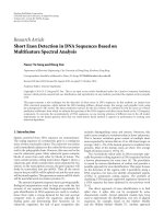
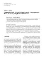
Figure 1: Structure of the proposed neuro-fuzzy fatigue recogni-
tion model.
crossing point between the two modulus maxima at each
scale [42–44]. Consequently, the zero crossing point at the
scale 2
4
is taken as the R-wave peak point [42–44], which re-
sults in HRV. Then, WT with a Haar wavelet function was
performed on HRV, and the result is such that the sum of
wavelet decomposition coefficientsat1and2levelscorre-
sponds to LF, and the sum of wavelet decomposition coeffi-
cients at 3 and 4 levels corresponds to HF [45]. Therefore we
can get the LF/HF ratio.
Under a normal condition, the LF/HF ratio is calculated
as the standard baseline, and the differences between the
baseline and the current LF/HF ratio is calculated, symbol-
ized as z
5
.Denotey
4
as the driver’s probabilistic state corre-
sponding to z
5
.
2.5. EM analysis
Eye activity which can be characterized by the percentage of
eye closure over a given time is one of the visual behaviors

that reflect a driver’s fatigue level. This can be demonstrated
by the previous studies [1, 46] that the driver maybe is in fa-
tigue as the eyes are at least 80 percent closed in a given time,
and that PERCLOS has been found to be the most valid ocu-
lar parameter for monitoring fatigue. Therefore, the running
average of PERCLOS instead of PERCLOS (to ensure the ro-
bustness of the PERCLOS measurement) is accepted as a fea-
ture to describe fatigue in this study. We use the normalized
variable z
6
∈ [0, 1] to denote the running average of PER-
CLOS, and make the probabilistic variable y
5
correspond to
z
6
.
To o b t a i n z
6
, a CCD camera is fixed on the dashboard
of the Northeastern University’s virtual environments driver
simulator to focus on the driver’s face for detecting the mul-
tiple visual behaviors. The program continuously tracks the
driver’s pupil shape at each 2 seconds sampling time instance
to determine the eye state (openness/closure) (for details,
please refer to [1]). In a given time (e.g., 30 sec), if the driver’s
eyes are closed continuously for p (p
= 0, 1, , 15) sam-
pling time instances, and then z
6

= 2∗p/30.
2.6. Summary of the proposed structure
In the above analysis, the SQ and DH fall into the contextual
category, the EEG and ECG fall into the contact category, and
the EM falls into the contact-less category. As such, there are
five pair relations, namely, (z
i
, y
i
)(i = 1, 2, 3, 4, 5), and they
are gathered into the architecture of the neuro-fuzzy TSK
(Takagi-Sugeno-Kang) model [47] proposed in this study;
see Figure 1.Eachoutputy
i
only partially reflects driver’s fa-
tigue from a certain aspect, which is not reliable to the fatigue
measurement. OWA method is chose in this study to fuse the
five fuzzy output variables in order to make the final fatigue
measurement y
∈ [0, 1] more reliable.
3. THE NEURO-FUZZY TSK NETWORK MODEL
3.1. Neuro-fuzzy TSK structure
Figure 1 shows that there are 5 neuro-fuzzy TSK subnetworks
(named from TSK1 to TSK5) with different parameters but
the same structure. Each of them is viewed as a multi-input
and single output (MISO) fuzzy system (if a system has only
one input and one output, the system is viewed as a special
case of the MISO fuzzy system). Let us take one of the five
MISO fuzzy systems as an example to explain the structure
of the neuro-fuzzy TSK system.

Denote
y
= y
i
,
x
= z
i
= [x
1
, x
2
, , x
N
]
T
,
i
= 1, 2, 3, 4, 5
(3)
as the output value and input vector, respectively, where N is
the number of the inputs, and i denotes the ith TSK model;
i
= 1, 2, 3, 4, 5 in this case. Suppose that M inference rules
are available for the system. The general form of the kth (k
=
1, 2, , M) TSK inference rule can be stated as follows [27,
48–50],
Rule k :Ifx is A
k

then y = f
k
(x), (4)
where f
k
(x
1
, , x
N
) is a crisp output function, and A
k
is
a fuzzy set labeled by a linguistic description (e.g., small,
medium, or large).
The first question regarding (4) is how to specify the
fuzzy set A
k
. Generally speaking, the clustering techniques
such as the fuzzy c-means (FCM) algorithm [50], the moun-
tain method [51], and the hybrid clustering and gradient de-
scent (HCGD) approach [52]areeffective methods to get A
k
from the input-output data available. In this study, HCGD
with some modifications is taken because it can automati-
cally generate a number of clusters and classify all input data
points into different clusters without requiring any assump-
tions about the data points. The modified HCGD method
works as follows.
6 EURASIP Journal on Advances in Signal Processing
Suppose that there are Q samples. Denote the ith input-

output pair of samples as s
i
= (x
1
(i), x
2
(i), , x
N
(i), y(i))
T
(i = 1, 2, , Q). We have the following steps.
Step 1. Define Q number of vectors v
i
(i = 1, 2, , Q), and
let v
i
= s
i
(i.e., s
i
is the initial value of v
i
).
Step 2. Compute the potential function h
ij
(v
i
, v
j
)betweenv

i
and v
j
with the following equation:
h
ij
(v
i
, v
j
) = exp

−


v
i
−v
j


2
2α
2

,
i
= 1, 2, , Q, j = 1, 2, , Q,
(5)
where

v
i
−v
j

2
represents the Euclidean distance between
v
i
and v
j
,andα is the width of the Gaussian function which
is fixed by experiments.
Step 3. Calculate
v
i
(i = 1, 2, , Q) with the following equa-
tion:
v
i
=

Q
j
=1
h
ij
v
j


Q
j
=1
h
ij
,(6)
and check whether
v
i
is close enough to v
i
for i = 1, 2, , Q,
that is,
|v
i
− v
i
|≤ε, i = 1, 2, , Q
,(7)
where ε is a very small positive number which has strong re-
lations with the number of fuzzy sets and the computation
load. Generally speaking, the number of fuzzy sets and the
computation load increase with the decrease of ε.Inmost
applications, ε is chosen empirically or experimentally. If (7)
is satisfied, then go to the next step; otherwise, let v
i
= v
i
and
go to Step 2.

Step 4. The original data with the same convergent vector is
clustered into a cluster, and the number of convergent vectors
is equal to the number of clusters. The convergent vector is
the cluster center and expressed as
c
k
=

c
k1
, c
k2
, , c
kN

T
, k = 1, 2, , M.
(8)
Compared to the original HCGD [52], the modified HCGD
as presented above has the following unique features.
(1) In the whole iterative process, all of the potential func-
tion h
ij
is taken into account in (6)and(7)nomatter
how big or small it is. In this way we could avoid the sit-
uation where contribution of particular h
ij
to the con-
vergent vector is excluded when h
ij

is very small.
(2) A somewhat “hard” stop criterion is imposed (see (7))
so that any dead-loop in the algorithm can be avoided.
Given that each cluster is associated with one indepen-
dent inference rule, the centroid of each cluster is automat-
ically assigned to the center of the premise of the rule. Af-
ter the number of clusters is determined, one needs to spec-
ify the membership degree to which variable x belongs to
L1 = layer1
L2
= layer2
L3
= layer3
L4
= layer4
x
1
x
2
x
N
··· ··· ···
···
···
···
···
xx
x
y
L1

L2
L3
L4
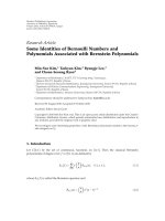
Figure 2: One-order neuro-fuzzy TSK network.
the fuzzy set A
k
. There are many types of membership func-
tions such as triangle-shape, trapezoidal-shape, bell-shape,
and Gaussian membership functions. In this study, the Gaus-
sian membership function was chosen because of its univer-
sal approximation and simple multidimensional decomposi-
tion [27, 49]. Thus, the premise (if x is A
k
)isdescribedas
μ
k
n
(x
n
) = exp

−

x
n
−c
kn

2
2σ

2
kn

, n = 1, 2, , N,
(9)
where σ
kn
is the width of the Gaussian membership function,
which is further determined by the following equation [52]:
σ
kn
=




−

N
m
=1
(x
∗
m
−c
km
)
2
2ln(u)
, n

= 1, 2, , N,
(10)
where x
∗
is the farthest data point from the cluster cen-
ter
c
k
,andu ∈ [0.1, 0.3] [52]. The procedure as described
above was implemented by the fuzzification corresponding
to the first layer of the neuro-fuzzy subnetwork, as shown in
Figure 2.
The second question regarding (4) is to determine the fir-
ing strength of the corresponding fuzzy rule. Let one node
represent one fuzzy logic rule in the second layer and the out-
put of the node represent the firing strength corresponding
to the fuzzy rule. In this study, the AND operator [27] is cho-
sen to determine the firing strength η
i
(x), that is,
η
k
(x) =
N

n=1
μ
k
n
(x

n
) = exp [−(D
k
(x − c
k
))
T
(D(x −c
k
))],
(11)
where D
k
= diag (1/σ
k1
,1/σ
k2
, ,1/σ
kN
), and c
k
= (c
k1
, c
k2
,
, c
kN
). The procedure as described above was implemented
by the second layer of the neuro-fuzzy subnetwork, as shown

in Figure 2.
G. Yang et al. 7
The first-order TSK crisp output function is often em-
ployed to get the result of f
k
(x
1
, , x
N
), which has the fol-
lowing form [49]:
f
k
(x
1
, , x
N
) = p
k0
+
N

n=1
p
kn
x
n
, (12)
where p
k0

, p
k1
, p
kN
, are crisp numbers adjusted at the
learning process. After having generated TSK functions f
k
,
the next step is to calculate the summation of f
k
with a nor-
malization procedure to produce the output y of TSK; see the
following equations below [27, 49],
y(x)
=
M

k=1
ω
k
f
k
(x)
=
M

k=1
ω
k


p
k0
+
N

n=1
p
kn
x
n

,
ω
k
=
η
k
(x)

M
m
=1
η
m
(x)
.
(13)
The procedure as described above was implemented by the
third and fourth layers of the neuro-fuzzy subnetwork, as
shown in Figure 2.

3.2. Parameter identification of
the neuro-fuzzy TSK network
After the structure of the neuro-fuzzy network model as de-
scribed above is generated from the given input-output data
pattern, the network parameters (i.e., the parameters in the
TSK functions and the parameters in the Gaussian function)
from the same input-output data pattern need to be deter-
mined. At this point, both feed-forward network and recur-
rent neural network can be used to achieve this purpose.
The recurrent neural network is more suitable for the prob-
lems with highly non-linear dynamics, but it is computa-
tionally overhead. The feed-forward network (e.g., the back-
propagationnetwork)hasextensivelybeenusedinthefield
of function approximation, pattern recognition, and pattern
classification because of its computational efficiency, but it
may have more chances to get a local minimum. The lo-
cal minimum problem can usually be resolved by carefully
selecting the initial weights of the neural network. Given
that the nature of our application, discussed in this paper, is
largely about the clustering and pattern recognition and the
application demands a fast response, the back-propagation
method is employed for learning in this study. In the fol-
lowing, several key steps of back-propagation algorithm for
learning are presented.
Denote y
d
(t)andy(t) as the desired and current outputs
of the network at time t, respectively. In order to obtain the
network parameters through learning, define a goal function
E as follows:

E
=
1
2
[y
d
(t) − y(t)]
2
. (14)
For the convenience of description, denote h
ζ
ξ
as the output
of the ξth node in the ζ th layer of the neuro-fuzzy network.
In the last layer (the fourth layer), denote h
4
1
= y(t)because
there is only one node in this layer. According to the back-
propagation method, the minimum of E corresponds to the
determination of the network parameters, which is done it-
eratively with the following equations [27]:
p
kn
(t +1)= p
kn
(t)+α[h
4
1
(t) − y

d
(t)]h
2
k
(t)x
n
,
p
k0
(t +1)= p
k0
(t)+α[h
4
1
(t) − y
d
(t)]h
2
k
(t),
c
kn
(t +1)=
c
kn
(t) −α
∂E
∂h
4
1

∂h
4
1
∂h
3
k
∂h
3
k
∂h
2
k
∂h
2
k
∂h
1
k
∂h
1
k
∂c
kn
,
σ
kn
(t +1)= σ
kn
(t) −α
∂E

∂h
4
1
∂h
4
1
∂h
3
k
∂h
3
k
∂h
2
k
∂h
2
k
∂h
1
k
∂h
1
k
∂σ
kn
,
(15)
where α is the learning rate.
4. SENSOR FUSION TECHNIQUE

4.1. Features available
As shown in Figure 1, SQ, DH, EEG, ECG, and EM are
fed into neuro-fuzzy networks of TSK1, TSK2, TSK3, TSK4,
and TSK5, respectively, resulting in the network outputs
y
i
(i = 1, 2, ,5), denoted as o = [y
1
, y
2
, y
3
, y
4
, y
5
]
T
.Let
w
= [w
1
, w
2
, w
3
, w
4
, w
5

]
T
denote the associated weight vec-
tor. Construct b
= [b
1
, b
2
, b
3
, b
4
, b
5
]
T
such that b
i
(i =
1, 2, , 5) is the ith largest element of the collection of
y
1
, y
2
, y
3
, y
4
,andy
5

. According to the OWA method [33], y
can be calculated by
y
= w
T
b =
5

i=1
w
i
b
i,
0 ≤ w
i
≤ 1, i = 1, 2, ,5,
5

i=1
w
i
= 1.
(16)
A number of techniques [28, 50, 53–55]areavailabletode-
termine the weight vector w of (16).Inthisstudy,wetakea
combined technique from the literature [53, 55].
Let
w ={w
i
(i = 1,2, ,5)}be the estimation of w,and

specify [53]
w
i
=
e
λ
i

5
j
=1
e
λ
j
,
i
= 1, 2, ,5.
(17)
In order to ensure the constraints of 0
≤ w
i
≤ 1(i =
1, 2, ,5) and


w
i
= 1, λ
i
is taken as the unknown pa-

rameter to be determined in the learning process. There
are k outputs of the neuro-fuzzy TSK network, denoted by
o
k
= [y
k1
, y
k2
, y
k3
, y
k4
, y
k5
]
T
(k = 1, 2, , K). According to
OWA [33], we will reorder o
k
to b
k
= [b
k1
, b
k2
, b
k3
, b
k4
, b

k5
]
T
,
where b
ki
is the ith largest element of the collection
of y
k1
, y
k2
, y
k3
, y
k4
, y
k5
.Lety
k
d
be the current estimated
8 EURASIP Journal on Advances in Signal Processing
aggregatedvalues corresponding to b
k
and w.Then,y
k
d
can
be calculated by
y

k
d
= w
T
b
k
=
5

i=1
w
i
b
ki
=
b
k1
e
λ
1

5
j
=1
e
λ
j
+
b
k2

e
λ
2

5
j
=1
e
λ
j
+ ···+
b
k5
e
λ
5

5
j
=1
e
λ
j
.
(18)
Let y
k
d
be the expected aggregated values corresponding to o
k

,
then the error e
k
between y
k
d
and y
k
d
can be calculated by
e
k
=
1
2

y
k
d
−
y
k
d

2
=
1
2

5


i=1
w
i
b
ki
−
y
k
d

2
.
(19)
Using the steepest gradient descent method [53], the param-
eters λ
i
(i = 1, 2, , 5) are updated with the following equa-
tion:
λ
i
(k +1)= λ
i
(k) −2βw
i
(b
ki
− y
k
d

)e
k
, (20)
where β is the learning rate. Consequently, parameters w
i
are
calculated at each iteration step for the current values of pa-
rameters λ
i
(k)(i = 1, 2, ,5).
4.2. Features unavailable
We consider two situations where some features are not avail-
able: (1) one feature is not available, and (2) two features are
not available. In Situation (1), suppose that a particular fea-
ture τ(1
≤ τ ≤ 5) is not available. Then, (18)canberewritten
as
y
k
d
= ( w

)
T
b

k
=
5


i=1,i=τ
w

i
b

ki
, (21)
where
w

={w

i
(i = 1, 2, ,5, and i=τ)} which should
be obtained through retraining, b

k
={b

ki
(i = 1, 2, ,5,
and i
=τ)}
T
; and at last, the final estimated output y
k
d
of the
system can be calculated by

y
k
d
= y
k
d
∗(1 − w
τ
), (22)
where
w
τ
∈{w
i
(i = 1, 2, ,5)},and(1− w
τ
) stands for the
belief function in the case that one feature is not available.
In Situation (2), suppose that two features τ and ξ(1
≤
τ, σ ≤ 5, and τ=σ) are not available. Then, (18)canberewrit-
ten as
y
k
d
= ( w

)
T
b


k
=
5

i=1,i=τ,i=σ
w

i
b

ki
, (23)
where
w

={w

i
(i = 1,2, ,5,and i=τ, i=σ)} which
should be obtained through retraining, b

k
={b

ki
(i = 1, 2,
,5, and i
=τ, i=σ)}
T

; and at last, the final estimated output
y
k
d
of the system can be calculated by
y
k
d
= y
k
d
∗(1 − w
τ
− w
σ
), (24)
where
w
τ
, w
σ
∈{w
i
(i = 1, 2, ,5)},and(1− w
τ
− w
σ
) stands
for the belief function in the case that two features are not
available. Note that if more than two features are not avail-

able, the same procedure can be designed.
5. THE SIMULATION-BASED EXPERIMENT
In order to demonstrate the validity of the TSK-OWA
method, we first perform training on a set of data obtained
from the subjects who participated in an experiment to de-
termine both the structure and parameters of the TSK-OWA.
Then, another set of data obtained from the subjects under
different simulation situations is obtained and performed on
the TSK-OWA with the trained structure and parameters to
illustrate the effectiveness of the TSK-OWA approach.
5.1. Experiment setup
Referring to the experimental conditions for producing the
contact-feature datasets of ECG and EEG [7, 8, 20, 39–
45, 54], and the contact-less-feature dataset of EM [1, 56], we
designed an experiment environment to acquire necessary
data based on Northeastern’s virtual environments driver
simulator. The simulator is equipped with the instruments
such as CCD camera, eye gaze tracking, and one for acquir-
ing EEG and ECG signals.
5.2. Data acquisition
To get the dataset of SQ, we designed a questionnaire ac-
cording to the experimental conditions for producing the ca-
sual dataset of SQ [4, 6, 38], mainly concerning the effec-
tive required sleep hours. The questionnaires are distributed
among the 9 driver participants and query them to answer
the question of how many effective hours they sleep at night
before participating the experiment.
To get the datasets of EEG, ECG, and EM, the 9 driver
participants are asked to participate in the experiment. Each
of them sat in front of the monitor with his hands on the

steering wheel to control the car running at the speed of 80
kilometer/hour and staying in the center of the simulated
freeway. At the same time, EEG and ECG signals of each
participant are measured at the sampling rate of 250 HZ,
and his/her dynamical facial image is obtained at the sam-
pling rate of 2 seconds. EEG and ECG signals and a series of
dynamical facial image are processed with the method pre-
sented in Section 2.Asaresult,nicedatasetsofEEG,ECG,
EM, and DH are obtained and normalized. Seven drivers
were randomly selected from the nine participants, along
with their datasets, are used for training, and the remaining
two drivers are for the algorithm evaluation.
5.3. Implementation of the neuro-fuzzy
TSK network model
In this study, 7 datasets are taken as the inputs of TSK1,
TSK2, TSK3, TSK4, and TSK5, and α
2
and ε are set to be 0.08
and 0.01, respectively. Under these conditions, each input
G. Yang et al. 9
00.10.20.30.40.50.60.70.80.91
Input
= SQ
0
0.1
0.2
0.3
0.4
0.5
0.6

0.7
0.8
0.9
1
Output = y
1
Input sample
Centroid of the clustering
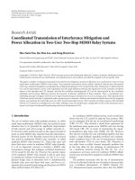
Figure 3: SQ input space partition for TSK1.
00.10.20.30.40.50.60.70.80.91
Input
= DH
0
0.1
0.2
0.3
0.4
0.5
0.6
0.7
0.8
0.9
1
Output = y
2
Input sample
Centroid of the clustering
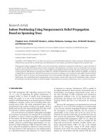
Figure 4: DH input space partition for TSK2.
space for TSK1, TSK2, TSK3, TSK4, and TSK5 is partitioned,
as shown in Figures 3–7.

From Figure 3, it can be seen that the SQ input space
is automatically partitioned into three fuzzy sets. Thus, the
neuro-fuzzy TSK1 network has three fuzzy inference rules
corresponding to the three fuzzy sets. The premise and con-
sequent parameters of the inference, denoted as c
1
i
(i =
1, 2, 3) and, p
1
ij
(i = 1, 2, 3, j = 0, 1), respectively, are de-
termined by training with the same given training samples,
and they are listed in Tab le 1.
From Figure 4, it can be seen that the DH input space
is automatically partitioned into three fuzzy sets. Thus, the
neuro-fuzzy TSK2 network has three fuzzy inference rules
corresponding to the three fuzzy sets. The premise and con-
sequent parameters of the inference, denoted as c
2
i
(i =
1, 2, 3) and p
2
ij
(i = 1, 2, 3, j = 0, 1), respectively, are de-
termined by training with the same given training samples,
as shown in Ta bl e 2 .
10.80.60.40.20
Input

= changes of θ
0
0.2
0.4
0.6
0.8
1
Input
=
changes of α
0
0.2
0.4
0.6
0.8
1
Output = y
3
Input sample
Centroid of the clustering
Figure 5: EEG input space partition for TSK3.
00.10.20.30.40.50.60.70.80.91
Input
= ECG
0
0.1
0.2
0.3
0.4
0.5

0.6
0.7
0.8
0.9
1
Output = y
4
Input sample
Centroid of the clustering
Figure 6: ECG input space partition for TSK4.
00.10.20.30.40.50.60.70.80.91
Input
= EM
0
0.1
0.2
0.3
0.4
0.5
0.6
0.7
0.8
0.9
1
Output = y
5
Input sample
Centroid of the clustering
Figure 7: EM input space partition for TSK5.
10 EURASIP Journal on Advances in Signal Processing

Table 1: Parameters for TSK1.
c
1
1
c
1
2
c
1
3
0.9046 0.5007 0.0970
p
1
10
p
1
20
p
1
30
1.0036 0.9504 0.9947
p
1
11
p
1
21
p
1
31

−1.0028 −0.8934 −0.9915
Table 2: Parameters for TSK2.
c
2
1
c
2
2
c
2
3
0.2035 0.5907 0.9217
p
2
10
p
2
20
p
2
30
0.0498 −0.0481 −0.1812
p
2
11
p
2
21
p
2

31
0.9216 1.1005 1.1814
Table 3: Parameters for TSK3.
c
3
11
c
3
12
c
3
21
c
3
22
c
3
31
c
3
32
0.202 0.182 0.492 0.482 0.846 0.852
P
10
P
11
P
12
0.01 0 0
P

20
P
21
P
22
0.3443 0.0957 0.2087
P
30
P
31
P
32
0.8476 0.0324 0.0364
From Figure 5, it can be seen that the EEG input space
is automatically partitioned into three fuzzy sets. Thus the
neuro-fuzzy TSK3 network has three fuzzy inference rules
corresponding to the three fuzzy sets. The premise and con-
sequent parameters of the inference, denoted as c
3
ik
(i =
1, 2, 3, k = 1, 2) and p
3
ij
(i, j = 1, 2, 3, j = 0, 1, 2), respec-
tively, are determined by training with the same given train-
ing samples, as shown in Ta bl e 3 .
From Figure 6, it can be seen that the ECG input space
is automatically partitioned into three fuzzy sets. Thus, the
neuro-fuzzy TSK4 network has three fuzzy inference rules

corresponding to the three fuzzy sets. The premise and con-
sequent parameters of the inference, denoted as c
4
i
(i =
1, 2, 3) and p
4
ij
(i = 1, 2, 3, j = 0, 1), respectively, are deter-
mined by training with the same given training samples, as
shown in Ta bl e 4 .
From Figure 7, it can be seen that the EM input space
is automatically partitioned into three fuzzy sets. Thus, the
neuro-fuzzy TSK5 network has three fuzzy inference rules
corresponding to the three fuzzy sets. The premise and con-
sequent parameters of the inference, denoted as c
5
i
(i =
1, 2, 3) and p
5
ij
(i = 1, 2, 3, j = 0, 1), respectively, are deter-
mined by training with the same given training samples, as
shown in Ta bl e 5 .
Table 4: Parameters for TSK4.
c
4
1
c

4
2
c
4
3
0.2305 0.5634 0.8925
p
4
10
p
4
20
p
4
30
0.0233 −0.1656 0.8339
p
4
11
p
4
21
p
4
31
0.06737 1.2597 0.092
Table 5: Parameters for TSK5.
c
5
1

c
5
2
c
5
3
0.179 0.5204 0.9209
p
5
10
p
5
20
p
5
30
0.0435 −0.0617 0.6533
p
5
11
p
5
21
p
5
31
0.2834 0.4755 0.2767
Table 6: Training samples for OWA.
y
1

y
2
y
3
y
4
y
5
y
d
0.1 0.2 0.2 0.3 0.1 0.18
0.3 0.5 0.45 0.5 0.2 0.39
0.2 0.3 0.2 0.1 0.4 0.24
0.92 0.85 0.8 0.9 0.95 0.884
0.8 0.7 0.65 0.73 0.9 0.756
0.92 0.96 0.94 0.9 0.91 0.926
··· ··· ··· ··· ··· ···
Table 7: Parameters for OWA.
w
1
w
2
w
3
w
4
w
5
0.1769 0.1955 0.2161 0.2161 0.1955
5.4. Implementation of the OWA method

When Outputs of TSK1, TSK2, TSK3, TSK4, and TSK5
(y
i
, i = 1, 2, , 5) are available, they are taken as the in-
puts of OWA and fed into OWA to be fused into the final
decision (i.e., fatigue estimation). In this study, training data
were selected to have a large coverage of possible cases. Some
training data pairs (i.e., y
i
and the expected aggregated value
y
d
) are shown in Ta bl e 6 .
The parameters of OWA are obtained through training
with the data as shown in Ta b le 6 . The training results are
listed in Tab le 7.
When some outputs of TSK1, TSK2, TSK3, TSK4, and
TSK5 (y
i
, i = 1,2, , 5) are not available, the structure and
parameters of OWA should be adjusted through retraining
with the dataset of the features not available. Some training
data pairs with features not available are shown in Tables 8,
9,and10, and the training results are listed in Tables 11, 12,
and 13.
G. Yang et al. 11
Table 8: Training samples for OWA with SQ not available.
y
2
y

3
y
4
y
5
y
d
0.96 0.94 0.9 0.91 0.9272
0.5 0.45 0.5 0.2 0.3625
0.2 0.2 0.3 0.1 0.2
0.85 0.8 0.9 0.95 0.875
0.3 0.2 0.1 0.4 0.25
0.7 0.65 0.73 0.9 0.745
0.2 0.2 0.3 0.5 0.3
··· ··· ··· ··· ···
Table 9: Training samples for OWA with EM not available.
y
1
y
2
y
3
y
4
y
d
0.2 0.3 0.2 0.4 0.275
0.92 0.85 0.8 0.9 0.8675
0.3 0.5 0.45 0.5 0.4375
0.1 0.2 0.2 0.3 0.2

0.8 0.7 0.65 0.73 0.756
0.65 0.51 0.32 0.78 0565
0.92 0.96 0.94 0.9 0.93
0.25 0.4 0.87 0.65 0.5425
··· ··· ··· ··· ···
Table 10: Training samples for OWA with SQ and EM not available.
y
2
y
3
y
4
y
d
0.7 0.65 0.73 0.693
0.3 0.2 0.1 0.20
0.5 0.45 0.5 0.483
0.85 0.8 0.9 0.85
0.96 0.94 0.9 0.90
0.2 0.2 0.3 0.233
0.65 0.78 0.63 0.687
0.55 0.69 0.34 0.527
··· ··· ··· ···
Table 11: Parameters for OWA with SQ not available.
w
2
w
3
w
4

w
5
0.2375 0.2625 0.2625 0.2375
5.5. Results and discussions
In order to test the structure and parameters of the pro-
posed TSK-OWA method, the remaining two drivers of the 9
participants did experiments under different conditions. For
the first driver, he had an insufficient sleep (e.g., 2 hours)
prior to driving and was asked to drive along a straight and
flat freeway in the simulated driving experiment for 2 hours
without stop. For the second driver, he had a sufficient sleep
(e.g., 7 hours) prior to driving, and was asked to drive along
a straight and flat freeway in the simulated driving experi-
ment for 2 hours without stop. At last, the first driver was in
fatigue state, while the second driver was in no-fatigue state
Table 12: Parameters for OWA with EM not available.
w
1
w
2
w
3
w
4
0.2199 0.2430 0.2686 0.2686
Table 13: Parameters for OWA with SQ and EM not available.
w
2
w
3

w
4
0.3115 0.3443 0.3442
Table 14: Features and simulation results for the first driver.
Input features
SQ DH ECG EEG EM
0.25 0.5 0.83 0.81 0.85 0.82
TSK output
y
1
y
2
y
3
y
4
y
5
0.9046 0.5907 0.8925 0.849 0.89
OWA fused result 0.8258
Final fused result 0.8258
Table 15: Features and simulation results for the second driver.
Input features
SQ DH ECG EEG EM
0.875 0.167 0.33 0.38 0.41 0.43
TSK output
y
1
y
2

y
3
y
4
y
5
0.075 0.21 0.29 0.33 0.41
OWA fused result 0.2598
Final fused result 0.2598
after finishing the driving experiment. In the whole driving
experiment, EEG and ECG signals, and a series of dynamical
facial image of the two drivers were recorded and processed
with the method presented in Section 2 to obtain datasets of
EEG,ECG,EM,andDH.
All datasets are fed into TSK1, TSK2, TSK3, TSK4, and
TSK5, and the outputs (y
i
, i = 1, 2, , 5) of the 5 TSK net-
works can be calculated by use of the parameters shown in
Ta bl es 1–5.
The outputs (y
i
, i = 1, 2, , 5) are fused into the fi-
nal output of the system by use of the parameters shown as
Ta bl e 7 . All simulated experiment results including the inter-
mediate and final computing are shown in the Tab le 1 4 (for
the first driver) and Tab le 15 (for the second driver).
When SQ feature is not available, outputs of TSK2, TSK3,
TSK4, and TSK5 (y
i

, i = 2, , 5) are fused into the output
of the system by use of the parameters shown in Tab le 11 ,and
then the final output of the system is calculated with (22).
All experiment results, including the intermediate and final
computing for the first driver, are shown in the Ta bl e 1 6.
When EM feature is not available, Outputs of TSK1,
TSK2, TSK3, and TSK4 (y
i
, i = 1, 2, , 4) are fused into
the output of the system by use of the parameters shown in
Ta bl e 1 2, and then the final output of the system is calculated
with (22). All experiment results, including the intermedi-
ate and final computing for the first driver, are shown in the
Ta bl e 1 7.
When SQ and EM features are not available, Outputs
of TSK2, TSK3, and TSK4 (y
i
, i = 2, , 4) are fused into
the output of the system by use of the parameters shown in
12 EURASIP Journal on Advances in Signal Processing
Table 16: Features and simulation result for the first driver when
SQ is not available.
Input features
SQ DH ECG EEG EM
— 0.5 0.83 0.81 0.82 0.82
TSK output
y
1
y
2

y
3
y
4
y
5
— 0.5907 0.8925 0.859 0.89
OWA fused result 0.8113
Final fused result 0.6677
Table 17: Features and simulation result for the first driver when
EM is not available.
Input features
SQ DH ECG EEG EM
0.25 0.5 0.83 0.81 0.85 —
TSK output
y
1
y
2
y
3
y
4
y
5
0.9046 0.5907 0.8925 0.859 —
OWA fused result 0.8052
Final fused result 0.6478
Table 18: Features and simulation result for the first driver when
SQ and EM are not available.

Input features
SQ DH ECG EEG EM
— 0.5 0.83 0.81 0.85 —
TSK output
y
1
y
2
y
3
y
4
y
5
— 0.5907 0.8925 0.859 —
OWA fused result 0.7771
Final fused result 0.4877
Ta bl e 1 2, and then the final output of the system is calculated
with (24). All experiment results including the intermediate
and final computing for the first driver are shown in Ta bl e 1 8.
From Ta bl e 1 4, it can be obviously seen that the final
output of the system is 0.8258, which means the probability
of the driver who is in the fatigue state is 82.58%. In other
words, it is obvious that the driver is in the most fatigue
state. This is consistent with the fact that the first driver is
in complete fatigue state after finishing the driving experi-
ment. From Ta b le 1 5 , it can be obviously seen that the final
output of the system is 0.2598, which means the probability
of the driver who is in the fatigue state is 25.98%. In other
words, it is obvious that the driver is in the nonfatigue state.

This is consistent with the fact that the second driver is in
nonfatigue state after finishing the driving experiment. The
results obtained as above demonstrate the effectiveness of the
TSK-OWA method.
From Tables 16–18, it can be also seen that the proba-
bility of the driver fatigue state for the same driver in the
same situation decreases with the decrease in the number of
features, which means that the recognition reliability of the
driver fatigue state decreases with the decrease in the number
of features. This implies that it is necessary to fuse multiple
features as many as possible in order to make fatigue recog-
nition more reliable when dealing with the driver’s fatigue
recognition problem.
6. CONCLUSIONS
This paper proposed a new method for inferring human cog-
nitive states based on multimodality cues. The method is
based on the integration of the neuro-fuzzy TSK network
and the multifeature fusion OWA. This new method is called
TSK-OWA. We presented an experimental validation in a vir-
tual driving simulator. The study can conclude.
(1) The classification of features into three different cat-
egories, namely, (1) contextual, (2) contact, and (3)
contact-less, adds value to the accuracy of inferring the
driver fatigue.
(2) A high coverage of features over these three categories
tends to improve the reliability of the measurement for
the driver fatigue.
(3) More cues appear to be more accurate in inferring the
drive fatigue.
One limitation with this work is that all the experimental

data were drawn from the simulator in the laboratory envi-
ronment instead from the real driving environment. There-
fore, a further experiment in a real driving environment is
one interesting future work. Another limitation is that still
only a few features are considered; more features need to
be studied in order to have a complete picture of the driver
fatigue state—which is an interesting future work. Further-
more, there is a need to perform sensitivity analysis with
regard to adding or dropping features. Finally, although it
seems feasible to generalize the conclusions drawn for infer-
ring the driver fatigue to any other cognitive state, including
emotion and mental workload, a future study seems to be
necessary for applying the proposed method to infer some
other cognitive and emotion states.
ACKNOWLEDGMENTS
The authors would like to acknowledge the generous finan-
cial support from Northeastern University (through a start-
up fund) and Natural Sciences and Engineering Research
Council (NSERC) of Canada (through a discovery grant and
University Faculty Award program) awarded to the second
author.
REFERENCES
[1] Q. Ji, Z. Zhu, and P. Lan, “Real-time non-intrusive monitoring
and prediction of driver fatigue,” IEEE Transactions on Vehicu-
lar Technology, vol. 53, no. 4, pp. 1052–1068, 2004.
[2] B. Fasel and J. Luettin, “Automatic facial expression analysis: a
survey,” Pattern Recognition, vol. 36, no. 1, pp. 259–275, 2003.
[3] Q. Ji, P. Lan, and C. G. Looney, “A probabilistic framework
for modeling and real-time monitoring human fatigue,” IEEE
Transactions on Systems, Man and Cybernetics A, vol. 36, no. 5,

pp. 862–875, 2006.
[4] T. Oron-Gilad and D. Shinar, “Driver fatigue among military
truck drivers,” Transportation Research Part F,vol.3,no.4,pp.
195–209, 2000.
[5] G. Hamouda and F. F. Saccomanno, “Neural network model
for truck driver fatigue accident detection,” in Proceedings of
G. Yang et al. 13
the Canadian Conference on Electrical and Computer Engineer-
ing, vol. 1, pp. 362–365, Montreal, Quebec, Canada, Septem-
ber 1995.
[6] C. D. He and C. C. Zhao, “Evaluation of the critical value of
driving fatigue based on the fuzzy sets theory,” Environmental
Research, vol. 61, no. 1, pp. 150–156, 1993.
[7] S.K.L.Lal,A.Craig,P.Boord,L.Kirkup,andH.Nguyen,“De-
velopment of an algorithm for an EEG-based driver fatigue
countermeasure,” Journal of Safety Research, vol. 34, no. 3, pp.
321–328, 2003.
[8] R C. Wu, C T. Lin, S F. Liang, T Y. Huang, Y C. Chen, and
T P. Jung, “Estimating driving performance based on EEG
spectrum and fuzzy neural network,” in Proceedings of the IEEE
International Joint Conference on Neural Networks, vol. 1, pp.
585–590, Budapest, Hungary, July 2004.
[9] B. J. Wilson and T. D. Bracewell, “Alertness monitor using neu-
ral networks for EEG analysis,” in Proceedings of the IEEE Sig-
nal Processing Society Workshop on Neural Networks for Signal
Processing (NNSP ’00), vol. 2, pp. 814–820, Sydney, Australia,
December 2000.
[10] T. H. Linh, M. Stodolski, and S. Osowski, “On-line heart beat
recognition using Hermite polynomials and neuro-fuzzy net-
work,” IEEE Transactions on Instrumentation and Measure-

ment, vol. 52, no. 4, pp. 1224–1231, 2003.
[11] M. Lagerholm, C. Peterson, G. Braccini, L. Edenbrandt, and
L. S
¨
ornmo, “Clustering ECG complexes using Hermite func-
tions and self-organizing maps,” IEEE Transactions on Biomed-
ical Engineering, vol. 47, no. 7, pp. 838–848, 2000.
[12] R. W. Picard, E. Vyzas, and J. A. Healey, “Toward ma-
chine emotional intelligence: analysis of affective physiologi-
cal state,” IEEE Transactions on Pattern Analysis and Machine
Intelligence, vol. 23, no. 10, pp. 1175–1191, 2001.
[13] E. Vyzas and R. W. Picard, “Affective pattern classification,” in
Emotional and Intelligent: the Tangled Knot of Cognition, AAAI
Fall Symposium Series, Orlando, Fla, USA, October 1998.
[14] Q. Wang, J. Yang, M. Ren, and Y. Zheng, “Driver fatigue de-
tection: a survey,” in Proceedings of the 6th World Congress on
Intelligent Control and Automation (WCICA ’06), vol. 2, pp.
8587–8591, Dalian, China, June 2006.
[15] W B. Horng, C Y. Chen, Y. Chang, and C H. Fan, “Driver
fatigue detection based on eye tracking and dynamic template
matching,” in Proceedings of the IEEE International Conference
on Networking, Sensing and Control, vol. 1, pp. 7–12, Taipei,
Taiwan, March 2004.
[16] Y. Norimatsu, S. Mita, K. Kozuka, T. Nakano, and S. Ya-
mamoto, “Detection of the gaze direction using the time-
varying image processing,” in Proceedings of the 6th IEEE An-
nual Conference on Intelligent Transportation Systems, vol. 1,
pp. 74–79, Shanghai, China, October 2003.
[17] D J. Kim, Z. Bien, and K H. Park, “Fuzzy neural
networks(FNN)-based approach for personalized facial

expression recognition with novel feature selection method,”
in Proceedings of the 12th IEEE International Conference on
Fuzzy Systems (FUZZ ’03), vol. 2, pp. 908–913, St. Louis, Mo,
USA, May 2003.
[18] R. Grace, V. E. Byrne, D. M. Bierman, et al., “A drowsy driver
detection system for heavy vehicles,” in Proceedings of the
17th Digital Avionics Systems Conference (DASC ’98), vol. 2, pp.
I36/1–I36/8, Bellevue, Wash, USA, October-November 1998.
[19] />technology.html.
[20] S. K. L. Lal and A. Craig, “A critical review of the psychophys-
iology of driver fatigue,” Biological Psychology, vol. 55, no. 3,
pp. 173–194, 2001.
[21] P. Vysok
´
y, “Changes in car driver dynamics caused by fatigue,”
Neural Network W orld, vol. 14, no. 1, pp. 109–117, 2004.
[22] P. Vysok
´
y, “Central fatigue identification of human operator,”
Neural Network W orld, vol. 11, no. 5, pp. 525–535, 2001.
[23] Y. Lin, P. Tang, W. J. Zhang, and Q. Yu, “Artificial neural
network modelling of driver handling behaviour in a driver-
vehicle-environment system,” International Journal of Vehicle
Design, vol. 37, no. 1, pp. 24–45, 2005.
[24] C. Conati, “Probabilistic assessment of user’s emotions in edu-
cational games,” Applied Artificial Intelligence, vol. 16, no. 7-8,
pp. 555–575, 2002.
[25] X. Li and Q. Ji, “Active affective state detection and user as-
sistance with dynamic Bayesian networks,” IEEE Transactions
on Systems, Man, and Cybernetics A, vol. 35, no. 1, pp. 93–105,

2005.
[26] Y. Zhang, Q. Ji, and C. G. Looney, “Active information fusion
for decision making under uncertainty,” in Proceedings of the
5th International Conference on Information Fusion, vol. 1, pp.
643–650, Annapolis, Md, USA, July 2002.
[27] C F. Juang and C T. Lin, “An on-line self-constructing neu-
ral fuzzy inference network and its applications,” IEEE Trans-
actions on Fuzzy Systems, vol. 6, no. 1, pp. 12–32, 1998.
[28] G. Beliakov, “Methods of construction of OWA operators from
data,” in Proceedings of the 10th IEEE International Conference
on Fuzzy Systems, vol. 1, pp. 184–187, Melbourne, Australia,
December 2001.
[29] T. Calvo, R. Mesiar, and R. R. Yager, “Quantitative weights
and aggregation,” IEEE Transactions on Fuzzy Systems, vol. 12,
no. 1, pp. 62–69, 2004.
[30] D. Filev and R. R. Yager, “On the issue of obtaining OWA op-
erator weights,” Fuzzy Sets and Systems, vol. 94, no. 2, pp. 157–
169, 1998.
[31] M. O’Hagan, “Aggregating template or rule antecedents in
real-time expert systems with fuzzy set logic,” in Proceedings
of the 22nd Asilomar Conference Signals, Systems and Comput-
ers, vol. 2, pp. 681–689, Pacific Grove, Calif, USA, October-
November 1988.
[32] V. Torra, “Learning weights for weighted OWA operators,” in
Proceedings of the 26th Annual Confjerence of the IEEE Indus-
trial Elect ronics Society (IECON ’00), vol. 4, pp. 2530–2535,
Nagoya, Japan, October 2000.
[33] R. R. Yager, “On ordered weighted averaging aggregation op-
erators in multicriteria decision making,” IEEE Transactions
on Systems, Man and Cybernetics, vol. 18, no. 1, pp. 183–190,

1988.
[34] R. R. Yager, “OWA neurons: a new class of fuzzy neurons,” in
Proceedings of the International Joint Conference on Neural Net-
works (IJCNN ’92), vol. 1, pp. 226–231, Baltimore, Md, USA,
June 1992.
[35] R. R. Yager, “Modeling prioritized multicriteria decision mak-
ing,” IEEE Transactions on Systems, Man, and Cybernet ics B,
vol. 34, no. 6, pp. 2396–2404, 2004.
[36] R. R. Yager, “OWA aggregation over a continuous interval ar-
gument with applications to decision making,” IEEE Transac-
tionsonSystems,Man,andCyberneticsB,vol.34,no.5,pp.
1952–1963, 2004.
[37] A. Smiley, “Fatigue management: lessons from research,” in
Managing Fatigue in Transportation,L.Hartley,Ed.,pp.1–23,
Elsevier, Oxford, UK, 1998.
[38] P. Thiff
ault and J. Bergeron, “Monotony of road environment
and driver fatigue: a simulator study,” Accident Analysis & Pre-
vention, vol. 35, no. 3, pp. 381–391, 2003.
14 EURASIP Journal on Advances in Signal Processing
[39]T P.Jung,S.Makeig,M.Stensmo,andT.J.Sejnowski,“Es-
timating alertness from the EEG power spectrum,” IEEE
Transactions on Biomedical Engineering, vol. 44, no. 1, pp. 60–
69, 1997.
[40] J. C. Principe, S. K. Gala, and T. G. Chang, “Sleep staging au-
tomaton based on the theory of evidence,” IEEE Transactions
on Biomedical Engineering, vol. 36, no. 5, pp. 503–509, 1989.
[41] G. Calcagnini, G. Biancalana, F. Giubilei, S. Strano, and S.
Cerutti, “Spectral analysis of heart rate variability signal dur-
ing sleep stages,” in Proceedings of the 16th Annual Interna-

tional Conference of the IEEE Engineering in Medicine and Bi-
ology Society, vol. 2, pp. 1252–1253, Baltimore, Md, USA,
November 1994.
[42] C. Li, C. Zheng, and C. Tai, “Detection of ECG character-
istic points using wavelet transforms,” IEEE Transactions on
Biomedical Engineering, vol. 42, no. 1, pp. 21–28, 1995.
[43] J. P. Mart
´
ınez, R. Almeida, S. Olmos, A. P. Rocha, and P. La-
guna, “A wavelet-based ECG delineator evaluation on stan-
dard databases,” IEEE Transactions on Biomedical Engineering,
vol. 51, no. 4, pp. 570–581, 2004.
[44] J. S. Sahambi, S. N. Tandon, and R. K. P. Bhatt, “Using wavelet
transforms for ECG characterization. An on-line digital signal
processing system,” IEEE Engineering in Medicine and Biology
Magazine, vol. 16, no. 1, pp. 77–83, 1997.
[45] K. Murai, Y. Hayashi, and N. Wakabayashi, “Analysis of
heart rate variability of navigator at in/from ports by wavelet
transform,” in Proceedings of the IEEE Pacific Rim Confer-
ence on Communications, Computers and Signal Processing
(PACRIM ’01), vol. 2, pp. 681–685, Victoria, BC, Canada, Au-
gust 2001.
[46] W. W. Wierwille, L. A. Ellsworth, S. S. Wreggit, R. J. Fair-
banks, and C. L. Kim, “Research on vehicle-based driver sta-
tus/performance monitoring: development, validation, and
refinement of algorithms for detection of driver drowsiness,”
Administration Final Report: DOT HS 808 247, National
Highway Traffic Safety, 1994.
[47] S. Barada and H. Singh, “Generating optimal adaptive fuzzy-
neural models of dynamical systems with applications to con-

trol,” IEEE Transactions on Systems, Man and Cybernetics C,
vol. 28, no. 3, pp. 371–391, 1998.
[48] S. Abe and R. Thawonmas, “A fuzzy classifier with ellipsoidal
regions,” IEEE Transactions on Fuzzy Systems,vol.5,no.3,pp.
358–368, 1997.
[49] S. Osowski, T. H. Linh, and K. Brudzewski, “Neuro-fuzzy TSK
network for calibration of semiconductor sensor array for
gas measurements,” IEEE Transactions on Instrumentation and
Measurement, vol. 53, no. 3, pp. 630–637, 2004.
[50] M. Sugeno and T. Yasukawa, “Fuzzy-logic-based approach to
qualitative modeling,” IEEE Transactions on Fuzzy Systems,
vol. 1, no. 1, pp. 7–31, 1993.
[51] R. R. Yager and D. P. Filev, “Approximate clustering via the
mountain method,” IEEE Transactions on Systems, Man and
Cybernetics, vol. 24, no. 8, pp. 1279–1284, 1994.
[52] C C. Wong and C C. Chen, “A hybrid clustering and gradient
descent approach for fuzzy modeling,” IEEE Transactions on
Systems, Man, and Cybernetics B, vol. 29, no. 6, pp. 686–693,
1999.
[53] D. Filev and R. R. Yager, “Learning OWA operator weights
from data,” in Proceedings of the 3rd IEEE Conference on Fuzzy
Systems, IEEE World Congress on Computational Intelligence,
vol. 1, pp. 468–473, Orlando, Fla, USA, June 1994.
[54] J. A. Healey, “Wearable and automotive systems for affective
recognition from physiology,” Doctoral thesis, Massachusetts
Institute of Technology, Mass, USA, 2000.
[55] V. Torra, “Learning weights for weighted OWA operators,” in
Proceedings of the 26th Annual Confjerence of the IEEE Indus-
trial Elect ronics Society (IECON ’00), vol. 4, pp. 2530–2535,
Nagoya, Japan, October 2000.

[56] Y. Zhang and Q. Ji, “Active and dynamic information fusion
for facial expression understanding from image sequences,”
IEEE Transactions on Pattern Analysis and Machine Intelligence,
vol. 27, no. 5, pp. 699–714, 2005.