Báo cáo hóa học: " Research Article Prototype Implementation of Two Efficient Low-Complexity Digital Predistortion Algorithms" potx

Hindawi Publishing Corporation
EURASIP Journal on Advances in Signal Processing
Volume 2008, Article ID 473182, 15 pages
doi:10.1155/2008/473182
Research Article
Prototype Implementation of Two Efficient Low-Complexity
Digital Predistortion Algorithms
Ernst Aschbacher,
1, 2
Mei Yen Cheong,
3
Peter Brunmayr,
2
Markus Rupp,
2
and Timo I. Laakso
3, 4
1
MED-EL Medical Electronics, Research and Developement, F
¨
urstenweg 77a, 6020 Innsbruck, Austria
2
Institute of Communications and Radio-Frequency Engineering, Vienna University of Technology, 1040 Vienna, Austria
3
Signal Processing Laboratory, Helsinki University of Technology, 02150 Espoo, Finland
4
National Board of Patents and Registration of Finland, 00101 Helsinki, Finland
Correspondence should be addressed to Ernst Aschbacher,
Received 1 February 2007; Revised 10 August 2007; Accepted 16 September 2007
Recommended by S. Gannot
Predistortion (PD) lineariser for microwave power amplifiers (PAs) is an important topic of research. With larger and larger band-

width as it appears today in modern WiMax standards as well as in multichannel base stations for 3GPP standards, the relatively
simple nonlinear effect of a PA becomes a complex memory-including function, severely distorting the output signal. In this
contribution, two digital PD algorithms are investigated for the linearisation of microwave PAs in mobile communications. The
first one is an efficient and low-complexity algorithm based on a memoryless model, called the simplicial canonical piecewise
linear (SCPWL) function that describes the static nonlinear characteristic of the PA. The second algorithm is more general, ap-
proximating the pre-inverse filter of a nonlinear PA iteratively using a Volterra model. The first simpler algorithm is suitable for
compensation of amplitude compression and amplitude-to-phase conversion, for example, in mobile units with relatively small
bandwidths. The second algorithm can be used to linearise PAs operating with larger bandwidths, thus exhibiting memory effects,
for example, in multichannel base stations. A measurement testbed which includes a transmitter-receiver chain with a microwave
PA is built for testing and prototyping of the proposed PD algorithms. In the testing phase, the PD algorithms are implemented
using MATLAB (floating-point representation) and tested in record-and-playback mode. The iterative PD algorithm is then im-
plemented on a Field Programmable Gate Array (FPGA) using fixed-point representation. The FPGA implementation allows the
pre-inverse filter to be tested in a real-time mode. Measurement results show excellent linearisation capabilities of both the pro-
posed algorithms in terms of adjacent channel power suppression. It is also shown that the fixed-point FPGA implementation of
the iterative algorithm performs as well as the floating-point implementation.
Copyright © 2008 Ernst Aschbacher et al. This is an open access article distributed under the Creative Commons Attribution
License, which permits unrestricted use, distribution, and reproduction in any medium, provided the original work is properly
cited.
1. INTRODUCTION
Future mobile communication systems are intended to pro-
vide multimedia communications which require high-speed
broadband transmissions. These systems have to make effi-
cient use of the sparse and valuable spectrum while providing
reliable communication. Linear signaling such as high-order
quadrature amplitude modulation (QAM) is used as an effi-
cient means to fulfill the high data rate requirement. Orthog-
onal frequency division multiplexing (OFDM) modulation
is extensively employed and proposed for many broadband
systems (e.g., WLAN, WiMax [1, 2], LTE of 3GPP [3]) due
to its spectral efficiency and robustness in multipath envi-

ronments. The drawback of such schemes is their high peak-
to-average power ratio (PAPR), which requires the transmit-
ter system to be highly linear, especially the power amplifiers
(PAs), in order to avoid nonlinear distortion. Nonlinear am-
plification produces in-band, as well as out-of-band distor-
tion. While the increased error rate due to in-band distor-
tion can be reduced using error correction coding, linearisa-
tion techniques are needed in order to limit the out-of-band
power so that the stringent spectral mask requirements of
such communications systems can be met.
With the use of a linearisation technique, nonlinear dis-
tortion can be compensated while the PA is driven into
the nonlinear region to gain power efficiency. A remarkable
2 EURASIP Journal on Advances in Signal Processing
amount of research activities on linearisation techniques,
both in analogue and digital domains, are notable in the lit-
erature of the past two decades. Examples of analogue lin-
earisers are feedforward linearisation, Cartesian loop feed-
back lineariser [4] and PDs implemented using analogue
components [5–7]. Digital linearisers are mainly predistor-
tion based. In the late 1980s through the mid 1990s, many
look-up table (LUT) based digital PDs were proposed [8–10].
LUT-based designs are limited by the slow adaptation due to
their huge table size, especially when memory effects of the
PA are considered.
Another type of digital PD is based on parametric mod-
els, in which the PD is described, for example, by a Volterra
system [11], a polynomial function, a piecewise linear func-
tion or other PA model specific functions, such as the Saleh
model [12]. The number of adaptive parameters is signifi-

cantly reduced as compared to the LUT-based PD, so that
the hardware complexity can also be kept low. Digital PD is
advantageous compared to analogue schemes as it provides
more flexibility (e.g., future system changes are more easily
supported), and adaptivity is easy to incorporate. It is also
more robust, for instance, its linearisation performance does
not depend on difficult to tune analogue components as in
the feedforward linearisation method [4]. Digital PDs also
offer higher linearity, as well as better power efficiency and
cost effectiveness compared to their analogue counterparts.
Recently, digital baseband PDs have become more feasible
than before due to the rapid improvement of digital signal
processing (DSP) technology.
Most of the PDs proposed in the literature are validated
by computer simulations and the PA to be linearised is of-
ten an analytical or characteristic nonlinear function. How-
ever, implementation of the PD algorithm on hardware and
evaluation based on measurement of the actual linearisation
of a practical PA better decribes the behavior of a proposed
PD. There are only a handful of publications which con-
sidered hardware implementation and validation of the PDs
based on measurement of practical PAs. For example, [13–
16] reported implementation of LUT-based digital PDs on
DSP/FPGA hardware and validated on real PAs in measure-
ment testbeds. Another example of a partial hardware im-
plementation of a parametric model PD is reported in [17],
where the training algorithm of a memory polynomial PD is
implemented on a Texas Instruments’ floating-point digital
signal processor (TMS320C67xx). In [18] crest-factor reduc-
tion and digital predistortion are evaluated in a record-and-

playback fashion, but not using a fixed-point and real-time
hardware implementation. Also in [19] a memory polyno-
mial PD is evaluated on a PA in a record-and-playback mode.
In this paper, two parametric models, which are rather
different in their nature, are considered for modeling the
digital PDs. One is the simplicial canonical piecewise linear
(SCPWL) function, which is suitable for modeling memory-
less nonlinearities. The linear affine property of the SCPWL
function is exploited for developing a computationally ef-
ficient PD identification algorithm. The SCPWL PD pa-
rameters are identified without involving complex numer-
ical computation such as matrix inversion. Another is the
Volterra series that is suitable for modeling nonlinearities
with memory. As the pre-inverse of the Volterra model PA
is difficult to obtain analytically, iterative methods based on
the Newton-Raphson method and successive approximation
method are employed to identify the Volterra model PD.
The secant method instead of the standard Newton-Raphson
method is used in order to relax the requirement for an an-
alytic PA model and to reduce the computaional burden on
computing the step size. Convergence analysis by simulations
for these iterative methods is provided.
A measurement testbed was built for measuring, testing,
and prototyping of the PD algorithms. The nonlinear char-
acteristics of a test PA (Minicircuits MC-ZVE8G [20]) was
measured. The input-output data obtained by exciting the
test PA with a broadband multitone signal is used for iden-
tification of the PDs. Then the performance of the identified
PDs in linearising the test PA is evaluated by measurement.
The testbed also provides facilities for the chosen PD algo-

rithm to be implemented on digital hardware. An iterative
PD algorithm was implemented on an FPGA. Measurement
results prove excellent linearisation quality.
This paper is organized as follows. In Section 2,wemoti-
vate the need for PD linearisers in communications systems
and formulate the PD problem. Section 3 gives an overview
of the nonlinear models with and without memory consid-
ered for modeling the PA and PD in this paper. The proposed
PD algorithms are presented in Section 4 followed by the
setup of the measurement testbed in Section 5.InSection 6,
the linearisation performance of the PDs is evaluated in the
offline measurement mode. Section 7 discusses the FPGA
implementation of the iterative Volterra model PD. Measure-
ment results of the PD running in real-time on an FPGA are
presented in this section as well. Conclusions are drawn in
Section 8.
Notation
Discrete-time signal sequences are denoted by italic small cap
font with the time index denoted by n within square brack-
ets, for example, x[n]. Signal operators are denoted by upper-
case blackboard font, for example,
H{·} in y[n] = H{x[n]}.
The operator
H (generally a nonlinear operator in this pa-
per) transforms the signal x[n] into the signal y[n]. Scalar
functions are denoted by italic small cap font with argument
within parentheses, for example, f (
·). Vectors are in lower-
case boldface letters and matrices are in upper-case boldface
letters. Signals are in general complex-valued unless other-

wise stated.
2. MOTIVATION AND PROBLEM FORMULATION
Power efficiency and linearity of the power amplifier (PA)
are two equally important but contradicting requirements
in mobile communications systems. If the PA system in the
base station is operated inefficiently, the maintenance costs
and power consumption will become significantly higher and
the life span of the PA will also be reduced. Power efficiency
is particularly important in the mobile units for prolonging
the battery life. However, due to intrinsic properties, power
efficient PAs are nonlinear. Nonlinear distortion results in
Ernst Aschbacher et al. 3
in-band signal distortion and spectral regrowth in the am-
plified signal. These effects lead to increased bit-error rate at
the receiver and violation of regulatory specifications on ad-
jacant channel power (see, e.g., [21]).
The efficiency of a radio-frequency (RF) PA is usually
measured by the power-added efficiency (PAE)
η
=
P
RF,out
−P
RF,in
P
DC
,(1)
whereby P
RF,out
and P

RF,in
denote the RF output and RF in-
put powers of the PA, respectively, and P
DC
is the supplied
DC power. It measures how efficient DC power is converted
to RF output power, excluding the power due to the RF in-
put signal. In a system that transmits signals with fluctuating
envelope, for example, OFDM or CDMA signals, a signifi-
cant amount of power back-off (reducing P
RF,in
) is typically
required in order to limit nonlinear distortion caused by the
PA. However, when power back-off is imposed, power effi-
ciency is reduced. This can be observed from the simple re-
lationship in (1). When the input signal power is reduced,
the effective RF output power, that is, the numerator in (1),
decreases while P
DC
remains constant, leading to a reduced
PAE. The typical values of PAE achieved in today’s PAs for 3G
mobile communication base stations without linearisation
(operated in the linear region) are around 20%, whereas PAs
in handsets achieve around 40% efficiency [22]. Therefore,
in order to meet regulatory requirements on adjacent chan-
nel power and signal quality while operating the PA power
efficiently, linearisation techniques are required. In this pa-
per digital predistortion linearisers are considered.
2.1. Formulation of the predistortion problem
In designing the PD, the relationship between the nonlinear

system and the PD has to be established first. Figure 1 illus-
trates the discrete-time, baseband equivalent system of a pre-
distortion filter
P placed in cascade with a nonlinear system
N. The lower branch represents an ideal linear PA L where
the output is d[n]
= L{u[n]}=g·u[n − Δ]. The nonlinear
system
N may include the digital-to-analogue converter, I-Q
modulators, RF mixer, and most importantly the PA system
which may be of single or multiple stages. The predistortion
filter
P should be designed such that the output y[n]isas
close as possible to the linearly amplified (and delayed) ver-
sion of the input signal, that is,
y[n]
= N

P

u[n]

≈
d[n] = L{u[n]}=g·u[n −Δ].
(2)
Here, Δ denotes the introduced delay and g is the targeted
linear gain. Note that
P is the pre-inverse filter of N.Inorder
to identify the predistortion filter
P, the nonlinear system N

is first modeled and expressed as a nonlinear function. In this
paper two nonlinear functions, that is, the simplicial canon-
ical piecewise linear function and the Volterra series are em-
ployed for modeling
N. Then algorithms are deviced to find
the pre-inverse
P of these functions, that is, the PDs. The PD
identification algorithms are presented in Section 4.
N
P
L
u[n]
z[n]
y[n]
d[n]
Figure 1: Linearisation problem.
Next, a simplified description of how a digital PD is put
in operation in practice is given. Figure 2 shows a block di-
agram of a typical transmitter employing a digital predistor-
tion (DPD) system. The input signal u[n], consisting of the
in-phase I[n] and quadrature-phase component Q[n]ispre-
filtered by a nonlinear predistortion filter. After digital-to-
analogue conversion the signals modulate the carrier at the
transmit frequency f
c
. Before transmission, this analogue RF
signal is amplified by a power amplifier. Ideally, a feedback
path is used to feed the output signal back to the PD identifi-
cation algorithm in order to track the behaviour fluctuation
of the PA due to temperature variation, aging, or changing of

operational mode, for example, in multichannel PAs. Then,
the transmitted signal is a linearly amplified version of the
input signal if the PD is properly identified.
3. POWER AMPLIFIER MODELS
This section presents the two functions used in this work for
modeling the PA and subsequently the PD. First, the simpli-
cial canonical piecewise linear function (SCPWL) which is
suitable for modeling static nonlinearities is presented. Fol-
lowing, the Volterra series, which can be used to model non-
linearities with memory, is presented.
3.1. Static model: SCPWL function
A piecewise linear (PWL) function is a function that divides
the input space into a finite number of partitions, each de-
scribed by a linear affine function. Conventional PWL func-
tions are expressed region by region and thus require a huge
amount of coefficients. A compact form known as the canon-
ical PWL function was first introduced in [23]. It is expressed
as a global function with much fewer coefficients than the
conventional PWL function. More recently, the concept of
simplicial partition is used in [24] to develop PWL functions
in an even more compact form. This class of PWL functions
is known as the simplicial canonical piecewise linear (SCPWL)
functions. PWL functions have been used for modeling and
analysis of nonlinear circuits [25, 26] but are still uncommon
for modeling PA nonlinearities.
There are a few advantages of modeling static nonlin-
earities using a PWL function compared to a polynomial.
With proper partitioning of the input space, the PWL func-
tion can approximate strong nonlinearities (sharp compres-
sion/expansion) more accurately. It does not pose numeri-

calproblemssuchastheRungephenomenon[27] exhibited
4 EURASIP Journal on Advances in Signal Processing
I[n]
Q[n]
DPD
I
PD
[n]
Q
PD
[n]
I
out
[n]
Q
out
[n]
DAC
DAC
ADC
ADC
I-Q mod.I-Q de-mod.
Power amplifier
LO
f
c
AT T
y(t)
Figure 2: Concept of digital predistortion.
by high-order polynomials. Moreover, parameter estimation

for polynomials often involves inversion of a Vandermonde
matrix which is usually ill-conditioned. In the contrary, the
structure provided by the linear affine property of a PWL
function allows an efficient parameter estimation algorithm
which does not involve matrix inversion [28].
The SCPWL function [24]inR
1
with positive real input
r is expressed as
f
β
(r) = c
0
+
σ−1

i=1
c
i
λ
i
(r) = c
T
Λ
β
(r), (3)
where Λ
β
(r) = [1, λ
1

(r), , λ
σ−1
(r)]
T
is the basis function
vector and c
= [c
0
, , c
σ−1
]
T
is the SCPWL coefficient vec-
tor. The breakpoints β
= [β
1
, β
2
, , β
σ
]
T
are predefined and
can be chosen to optimally fit a given nonlinear function, σ
is the number of breakpoints. In (3), the subscript in Λ
β
(r)
and f
β
(r) indicates the chosen set of breakpoints for a given

nonlinearity that the SCPWL function is modeling. The ith
basisfunctionisgivenas
λ
i
(r) =
⎧
⎪
⎪
⎪
⎨
⎪
⎪
⎪
⎩
1
2

r −β
i
+


r −β
i



, r ≤ β
σ
,

1
2

β
σ
−β
i
+


β
σ
−β
i



, r>β
σ
.
(4)
The SCPWL function is suitable for modeling static non-
linearities such as AM/AM and AM/PM functions. Let the
baseband input and output signals be represented by z[n]
=
r
z
[n]e
jϕ
z

[n]
and y[n] = r
y
[n]e
j(ϕ
z
[n]+ϕ[n])
,wherer
z
[n]and
r
y
[n] denote the magnitude of the input and output signals,
respectively. Then the AM/AM and AM/PM conversions can
be approximated using two SCPWL functions as
f
r

r
z
[n]

=
r
y
[n] = c
T
r
Λ
β

r

r
z
[n]

,
f
ϕ

r
z
[n]

= ϕ[n] = c
T
ϕ
Λ
β
ϕ

r
z
[n]

,
(5)
where β
r
and β

ϕ
are the breakpoints vectors of the AM/AM
and AM/PM functions, respectively.
3.2. Dynamic model: Volterra series
The Volterra series is known as the most complete function
for describing dynamic nonlinear systems [29, 30]. It is a
functional power series of the form (if not specified, integra-
tion and summation limits are from
−∞ to ∞)
y(t)
= H{z(t)}
=
h
0
+
∞

p=1

···

h
p

t, τ
1
, , τ
p

×

z

τ
1

···z

τ
p

dτ
1
···dτ
p
,
(6)
in which
H is a nonlinear functional of the continuous func-
tion z(t), h
0
is a constant, t is a parameter, and h
p
(···), p ≥
1, are continuous functions, called the Volterra kernels. If
p
= 1 the Volterra series reduces to the input-output rep-
resentation of a simpler system:
y(t)
= h
0

+

h
1

t, τ
1

z

τ
1

dτ
1
. (7)
If furthermore h
0
= 0, a linear system is obtained and the
Volterra series reduces to a convolution. A Volterra series de-
scribes a large class of nonlinear systems, namely, all con-
tinuous nonlinear systems with fading memory [31]. Here,
a truncated and stationary Volterra series is used to model
the power amplifier. Taking into account the bandpass nature
of the power amplifier, the discrete-time complex baseband
Volterra model of the power amplifier is [32]
y[n]
= N{z[n]}
=
P−1


p=0
H
2p+1
{z[n]}=
P−1

p=0

n
2p+1
∈N
2p+1
h
2p+1
[n
2p+1
]
×
p+1

i=1
z

n −n
i

2p+1

i=p+2

z
∗

n −n
i

.
(8)
For notational compactness, the vector n
2p+1
= [n
1
, ,
n
2p+1
]
T
is used. This model can be easily simplified to the
static case (i.e., memoryless), where the kernels reduce to
scalars:
y[n]
= e
j arg {z[n]}
P−1

p=0
h
2p+1
|z[n]|
2p+1

= e
j arg {z[n]}
f

r
z
[n]

.
(9)
Ernst Aschbacher et al. 5
The (complex) nonlinear transformation can be rewritten as
f

r
z
[n]

=
f
r

r
z
[n]

e
jf
ϕ
(r

z
[n])
, (10)
with the AM/AM transformation f
r
(r
z
[n]) =|f (r
z
[n])| and
the AM/PM conversion f
ϕ
(r
z
[n]) = arg {f (r
z
[n])}.TheP
complex parameters h
2p+1
, p = 0, , P − 1, are the model
parameters and describe the AM/AM, as well as the AM/PM
conversion.
4. PREDISTORTION FILTERS
This section discusses the PD identification algorithms. A
non-iterative method known as the image coordinate map-
ping (ICM) method [28] is employed for identifying the
SCPWL PD. The ICM method is discussed in Section 4.1.
Two iterative methods are considered for approximating the
pre-inverse of the Volterra model PD, one based on the
Newton-Raphson method and the other is a successive ap-

proximation method. The iterative methods are presented in
Section 4.2 together with the analysis of their convergence
behaviour.
4.1. Identification of the SCPWL PD:
non-iterative solution
The ICM method is developed by exploiting the linear
affine property of the SCPWL function. The ICM method is
founded on the mirror image resemblance of the PA and PD’s
static nonlinearities along the unit linear gain line. When the
static nonlinearity of a PA is modeled using a PWL function,
each linear affine subregion is defined by a straight line con-
necting two coordinates. Based on this property, the PWL
subregions of the PD can be obtained by finding the mirror
images of the coordinates that define these linear affine func-
tions of the PA. The concept of vector projection (in this case,
reflection) using a transformation matrix is used in the ICM
method [28] for finding the PD coordinates.
Consider a unit desired linear gain at the output of the
PD-PA cascade. The transformation of b to the image coor-
dinates b

as shown in Figure 3(a) can be performed using a
2-by-2 antidiagonal matrix with the nonzero elements equal
one as

x

y



=

01
10

x
y

. (11)
This transformation swaps the input and output of the PA.
In effect, the mirror image connotes an inverse function of
the PA. However, in practice, the desired linear gain is rarely
chosen as one.
1
For non-unity linear gain, the PD function
is not an exact mirror image of the PA. The input-output re-
lation of the PD’s linear affine functions must also take into
account the desired linear gain g. This amplification factor
1
A reasonable choice of the desired linear gain is to choose a value that
leads to a maximum linearisation range, for example, up to the saturation
point of an AM/AM characteristic.
can be incorporated either by multiplying the output of the
PD by g or dividing the input of the PD by g. Notice that the
output space of the PD must coincide with the input space
of the PA. The gain must therefore be incorporated in the in-
put range of the PD. Thus, the ICM matrix for an arbitrary
desired linear gain g is given as
Q
=

⎡
⎢
⎣
0
1
g
10
⎤
⎥
⎦
. (12)
The PD coordinates are then obtained as
b

= Qb. (13)
Figure 3(b) shows an example of the nonlinear characteristic
of the SCPWL PD with respect to the PA characteristic when
g
= 1.2.
Once all the image coordinates b

k
(for k = 1, , σ)are
obtained, the breakpoints for the PD β

and the correspond-
ing amplitude responses f
β

(r = β


) are obtained. Substitut-
ing into (3), the SCPWL function for the PD can now be
written as
f
β


r
i
= β

i

=
Λ
T
β


r
i
= β

i

c

, (14)
where c


is the coefficients vector of the PD that needs to
be identified. By collecting (14)fori
= 1, , σ into matrix-
vector form, we have
f
β

(r = β

) = L
β

(r = β

)c

, (15)
where the matrix L
β

(β

) =

Λ
β

(β


1
), Λ
β

(β

2
), , Λ
β

(β

σ
)]
T
is the basis function matrix evaluated at the PD partition
points β

.
Note that L
β

(β

) is a nonsingular square matrix. The
inverse can be obtained by performing some linear opera-
tions on L
β

(β


). It is shown in [33] that its inverse L
I
(β

) ≡
L
β

−1
(β

) has nonzero elements only on the main diagonal
and two lower diagonals. Due to the linear affine property of
the SCPWL function, these nonzero elements can be com-
puted from the knowledge of the partition points β

. This
computation involves only subtractions and divisions. Thus,
the SCPWL PD coefficients can be obtained without invok-
ing matrix inversion as
c

= L
I
(β

)f
β


(β

), (16)
with low computational complexity.
4.2. Identification of the Volterra PD: iterative solution
As mentioned earlier, PD models are identified as the pre-
inverse of the PA model. In general, the pre-inverse systems
of nonlinear systems with memory, for example, the Volterra
model considered in this paper, are not easily determined an-
alytically. In [34] a method for the construction of the pth-
order pre-inverse filter for Volterra systems is introduced.
However, this method is rather complicated, which makes it
unsuitable for practical implementation. Instead of identify-
ing the model parameters of the PD, iterative methods can be
used to find the predistorted signals directly.
6 EURASIP Journal on Advances in Signal Processing
10.80.60.40.20
Input amplitude
Unit desired
linear gain
PD nonlinearity
PA nonlinearity
b

b
0
0.1
0.2
0.3
0.4

0.5
0.6
0.7
0.8
0.9
1
Output amplitude
(a)
10.80.60.40.20
Input amplitude
Desired linear gain
PD nonlinearity
PA nonlinearity
Coordinate projections
b
7
b
6
b

7
b

6
0
0.2
0.4
0.6
0.8
1

1.2
Output amplitude
(b)
Figure 3: Mirror image resemblance of PA and PD nonlinearities.
4.2.1. Root search: secant method
By reorganizing the relationship of the nonlinear system and
the PD in (2)to
N{z[n]}−g·u[n −Δ] = T
u
{z[n]}=0, (17)
the problem of finding the predistortion filter
P is reformu-
lated. The task is now to search the root z
∗
[n]of(17), which
is the output of the predistortion filter, see Figure 1.For
most nonlinear operators
N (here, N is the power amplifier
model), an analytic solution is not known. But the root z
∗
[n]
can be searched iteratively which gives an approximate solu-
tion. A common method to solve nonlinear equations, which
can also be applied to functionals, is the Newton-Raphson
method [35]. In this case the iterative algorithm reads
z
i+1
[n] = z
i
[n] −

1
∂
z
N {z
i
[n]}
T
u

z
i
[n]

, i ≥ 0. (18)
The advantage of the Newton-Raphson method is its rapid
convergence. In the neighbourhood of the solution, the
method converges with quadratic order. If ε
i
[n] =z
i
[n] −
z
∗
[n]/z
∗
[n] denotes the relative error at iteration-step i,
then
ε
i+1
[n]∼ε

i
[n]
2
. (19)
This rapid convergence is achieved at a high computational
cost since the reciprocal value of ∂
z
N{z
i
[n]} hastobecom-
puted. Convergence of the Newton-Raphson method cannot
be guaranteed but is generally achieved if the initial guess
z
0
[n] is not too far from the solution z
∗
[n].
Furthermore, notice that this method requires the
derivative of the PA model ∂
z
N to be evaluated at z
i
[n], that
is, the model has to be analytic. Most PA models, for ex-
ample, (8), are not analytic (see, e.g., the special case for
the static model (9)—the function
|z[n]| is analytic only at
z[n]
= 0). Since the Newton-Raphson method is not appli-
cable to the Volterra PA model, an alternative algorithm is

searched for. The Newton-Raphson step size can be approx-
imated using the secant method. In this case
T
u
{z[n]} need
not be analytic. The iterative secant algorithm reads
z
i+1
[n] = z
i
[n] −
z
i
[n] −z
i−1
[n]
N{z
i
[n]}−N{z
i−1
[n]}
T
u

z
i
[n]

,
i

≥ 0, z
−1
[n], z
0
[n]given.
(20)
The derivative ∂
z
N{z
i
[n]} is approximated with the secant.
The complexity is significantely reduced compared to the
standard Newton-Raphson method, since for the calculation
of the secant, only
N{z
i
[n]} has to be calculated. But this has
to be computed in any case for the calculation of
T
u
{z
i
[n]}
(cf. (17)).
Two initial values are needed. Since it is expected that
the solution is only slightly different from the input signal
(as long as the power amplifier is not heavily nonlinear), the
input signal z
0
[n] = u[n] is used. The second initial value

z
−1
[n] = 0, for simplicity. Also this algorithm is not guar-
anteed to converge. The convergence depends on the initial
values z
−1
[n]andz
0
[n]—if they are sufficiently close to the
solution the algorithm converges. It is shown, for example, in
[36], that the convergence rate is
ε
i+1
[n]∼ε
i
[n]
φ
, (21)
whereby φ
= (1/2)(1 +
√
5) ≈ 1.618 is the golden ratio. It
is slower than the convergence rate of the Newton-Raphson
Ernst Aschbacher et al. 7
method but can be improved if instead of z
i−1
[n]in(20)a
value closer to z
i
[n] is used, for example,

z
i−1
[n] = λz
i
[n]+(1−λ)z
i−1
[n], λ ∈ [0, 1). (22)
As λ approaches one, the derivative is better approximated
with the secant. For simplicity of the hardware realization,
the conventional secant algorithm with λ
= 0 is used in both
the offline MATLAB and the real-time FPGA implementa-
tions (see Sections 5–7).
4.2.2. Fixed-point s earch: successive approximation
The problem of determining the PD filter can be reformu-
lated in yet another way [37]. If the nonlinear model
N allows
for an additive decomposition, that is,
N{z[n]}=H
1
{z[n]} +
P−1

p=1
H
2p+1
{z[n]}, (23)
the problem (2) can be rewritten as a fixed-point equation in
z[n]as
z[n]

= H
−1
1

g·u[n − Δ] −
P−1

p=1
H
2p+1
{z[n]}

= S
u
{z[n]}.
(24)
The fixed-point z[n] is the output of the PD filter for the in-
put u[n]. This fixed-point is determined iteratively with the
method of successive approximation [35, 37]
z
i+1
[n] = S
u
{z
i
[n]}, i ≥ 0, z
0
[n]isgiven. (25)
This method can only be used if the problem can be brought
into a fixed-point equation in terms of z[n]. This is possi-

ble for models that allow for an additive decomposition like
(23) and where the first term
H
1
can be inverted, for example,
Volterra models with a linear part that can be inverted. Other
nonlinear models may not allow such a fixed-point formula-
tion.
The advantage of the successive approximation method
compared with the secant method is that the convergence
analysis can be performed using the contraction mapping
theorem [37]. It provides a sufficient condition for conver-
gence and states that the successive approximation converges
to the fixed-point if the operator
S
u
is contractive on a closed
set of a Banach space [35]. This convergence analysis is tech-
nically complex, for instance, the norms of the operators
H
2p+1
in (24) have to be determined in order to ascertain that
the operator
S
u
is contractive. In practice the norms can only
be upper-bounded, so that the analysis gives in general rather
conservative results which are often not very helpful in prac-
tice.
The convergence rate of successive approximation is lin-

ear, that is,
ε
i+1
[n]∼ε
i
[n], (26)
thus is much smaller than the convergence rate of the
Newton-Raphson or secant method. The consequence is
that more iterations have to be performed for achieving a
certain linearisation accuracy compared to the former two
methods, meaning that hardware complexity is increased.
In Section 4.2.3 it is shown by simulations that for a cer-
tain linearisation accuracy more iterations have to be per-
formed with successive approximation compared to the se-
cant method.
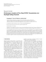
4.2.3. Convergence rate
In order to compare the convergence rate of the two meth-
ods, the secant method and the successive approximation, an
example Volterra model is linearised. The parameters of the
Volterra model are obtained using input/output data gen-
erated with an RF-circuit simulation using ADS [38]. The
simulated PA is a Motorola LDMOS amplifier (MRF21125).
Based on this data (WCDMA input signal, one channel) the
parameters of a Volterra model
N (cf. (8)) are estimated.
This assures that the example system to be linearised is re-
alistic. The Volterra model is of fifth-order and each ker-
nel has a memory length of two samples (sampling rate is
3.84 MHz
×8 = 30.72 MHz). In total 20 (complex) parame-

ters are necessary. The linearisation error is defined as
J
lin
(i)[dB] = 10 log


e
lin,i
[n]
2
2
d[n]
2
2

, (27)
with
e
lin,i
[n] = y
i
[n] −d[n] = N{z
i
[n]}−g·u[n − Δ], (28)
whereby z
i
[n] is calculated with the secant method (20)or
with successive approximation (25) and applied to the PA
model
N{·}. According to (21) the error decreases with every

iteration step by approximately 16 dB if the secant method is
used, whereas with successive approximation the error de-
creases with approximately 10 dB per iteration, correspond-
ing to the linear convergence behaviour of this method, see
(26). Figure 4 presents a graphical illustration.
Due to the slow convergence, the successive approxima-
tion method is too costly in terms of hardware rescources
for implementation in an FPGA. Therefore, only the se-
cant method is implemented. The successive approximation
method is presented here for comparison.
5. THE PROTOT YPING SYSTEM
In this work, the proposed PDs are designed using measure-
ment data obtained by exciting the Minicircuits MC-ZVE8G
[20] test PA with a broadband multisine signal. Then per-
formance of the PD algorithms on linearising the test PA is
evaluated by measurements. In this section, the setup of the
measurement testbed is first presented. Then, the two test
modes for testing the PD algorithms, namely, the offline test
and real-time test, are defined. The limitations of the mea-
surement testbed are also briefly discussed.
5.1. Measurement testbed
The testbed used in the work for measurements, testing, and
prototyping consists of a digital signal processing (DSP) part
8 EURASIP Journal on Advances in Signal Processing
4321
Number of iterations
Successive approximation
Secant method
−70
−60

−50
−40
−30
−20
−10
J
lin
(i)(dB)
Figure 4: Comparison of the convergence rate of the secant method
and the method of successive approximation.
and a radio frequency (RF) processing part. The DSP part is
built up with a host computer and DSP hardware, and the RF
part includes basic RF transceiver hardware and the test PA
MC-ZVE8G. In the following, the setup of these two parts is
detailed.
5.1.1. Digital signal processing part
Figure 5 illustrates the DSP part with hardware involved in
the testbed. The interface between the host computer and
the DSP hardware is provided by the Sundance SMT310Q
[39] peripheral component interface (PCI) card that carries
all DSP hardware on it.
Two Sundance SMT351-G memory modules [40]are
mounted on this carrier board, giving a total of 2 GB memory
for input-output (IO) data storage. The Sundance SMT370-
AC [41] module provides the ADC/DAC functions. This
module is equipped with the AD9777 [42]DACfromAna-
log Devices which implements also a digital I-Q modulator.
Using this I-Q modulator, the baseband signal is digitally
modulated onto an intermediate frequency (IF) carrier (cen-
ter frequency 70 MHz) before DA conversion. The Sundance

SMT370-AC module is also equipped with a Xilinx Virtex-
2 XC2V1000 FPGA [43], which allows a proposed PD algo-
rithm to be implemented and tested in real time.
The Sundance SMT365 digital signal processor (DSP)
module configures all other modules. It configures the
ADC/DAC and commands data transfer from the host com-
puter to the memory module and then to the SMT370-AC
module and vice versa. When the PD algorithm is imple-
mented on the FPGA, it sets the model parameters of the PD
filter on the FPGA after each update of the parameters set.
5.1.2. Radio frequency part
The block diagram of the RF part of the testbed is shown in
Figure 6. In the transmit path, an attenuator is placed before
the up-converter to reduce the power of the transmitted sig-
nal. This is done to minimize the nonlinear effect caused by
the up-converter. Then the signal is mixed to a center fre-
quency f
c
= 2.45 GHz and filtered. A preamplifier is used to
amplify the signal at the output of the up-converter to a suf-
ficient level. An adjustable attenuator is used to control the
input-power backoff (IBO) level of the signal to the test PA.
After the PA, the signal is fed back to the receive path.
Again, the output signal of the PA is attenuated to ensure
linearity of the down-converter. A common local oscillator
is used for both the up-converter and the down-converter
in order to avoid phase imbalance. The signal is down-
converted to IF and filtered. The IF signal is amplified before
the ADC so that the dynamic range of the ADC is optimally
utilized.

5.2. Test modes
In this work, the proposed PDs in Section 4 are first iden-
tified and tested using a synthetic PA model in MATLAB.
The linearisation performance is measured by the adjacent
channel power ratio (ACPR) of the PA output signal. In the
simulated environment, the power spectral density of the PA
output signal showed that the proposed PD algorithms to be
evaluated on a practical PA were successful in suppressing the
ACPR.
Next, the PD algorithms are brought to test on a practical
PA MC-ZVE8G on the testbed. A spectrum analyzer is used
to examine the linearisation performance based on the ACPR
of the PA output signal. The testbed supports two test modes
for testing the performance of the proposed PDs, namely, the
offline mode and the real-time mode. The configuration of
the RF part is common for the two test modes. In both test
modes, the nonlinear characteristics of the PA (modeled us-
ing an SCPWL function or a Volterra filter) are identified in
the host computer using algorithms implemented in MAT-
LAB. Different configurations in the DSP part that determine
the test mode are as follows.
In the offline mode, the PDs are also identified in the host
computer. Then, the input data is predistorted with the iden-
tified PD and transferred back to the memory module. In
this mode, the predistorted signal is computed using double-
precision floating-point arithmetic in MATLAB. From the
memory, the predistorted signal is transmitted directly to the
DAC and subsequently to the PA via the RF part. The FPGA
is bypassed. The offline test examines the PD performance in
a record-and-playback fashion. Both the SCPWL PD and the

Secant-Volterra PD are tested in this mode. The results of the
offline test are discussed in Section 6.
In the real-time mode, the PD algorithm is implemented
on the FPGA. The PA model parameters identified in the host
computer are transferred to the FPGA for implementation of
the PD filter. Then, the excitation signal data is sent to the
memory without being predistorted. From the memory, the
data is transmitted through the PD filter on the FPGA and
Ernst Aschbacher et al. 9
Tx signal upload
Memory
Mag.
Phase
Sundance SMT370
u[n]
Sundance SMT365
FPGA
DPD-filter
Model param. set
DSP
f
T
= 70 MHz
PCI bus
PC
To I / Q
f
T
= 70MHz
z

I
[n]
f
T
= 70MHz
z
Q
[n]
Model param.
estim. Matlab
4
×
Interp.
4
×
Interp.
Configure
PCI bus
2GBmemory
Sundance SMT351
DUC/DAC
DUC
f
m
= f
s
/4 = 70 MHz
16 bit
DAC
z(t)

f
s
= 280 MHz
ADC
y(t)14 bit
f
s
= 100 MHz
Figure 5:DSPpartofthetestbed.
From DAC
AT T
Digital part
To A D C
Pre-amplifier
Up-conv.
LO
Down-conv.
Driver amplifier
AT T
Power amplifier
AT T
Figure 6: RF part of the testbed.
predistorted in a real-time manner, see Figure 5. Then the
data is sent to the PA to examine the linearisation perfor-
mance. In this test mode, the predistorted signal is computed
using fixed-point precision. Note that the PA characteristic
is assumed to be varying very slowly. Thus, the PA model
is not updated continuously with every incoming data sam-
ple. The identification algorithm determines the PA model
in a block-based manner. In the real-time test mode, the PA

model is determined with the first block of IO data. In prac-
tice, the PA model can be updated with another block of IO
data whenever changes in the PA characteristic are detected,
for instance, due to aging or sudden changes of operation
mode (e.g., a new channel is added in multichannel applica-
tions). The FPGA implementation of the Secant-Volterra PD
and the real-time test results are presented in Section 7.
5.3. Limitations of the testbed
The testbed poses certain limitations in measurement of the
nonlinear PA characteristics due to the imperfection of the
available RF hardware.
As the up-converter and down-converter are nonlinear
devices, the power level of the signals before these devices
has to be attenuated. As a result, a low output signal level
is obtained. Thus, after up-conversion and down-conversion
preamplification is necessary to boost the signal to a suffi-
cient level to drive the test PA and for the signal to cover
a meaningful range of the ADC, respectively. However, the
preamplification increases the measurement noise floor. The
increased noise floor results in a smaller dynamic range, that
is, approximately 50 dB, as compared to 60 dB when mea-
surement is done before the down-converter. This is evident
in the measurements of the signal spectrum which are pre-
sented in the following two sections.
Another issue is due to the filters of the up-converter and
down-converter which are bandlimited to 20 MHz. In order
to model up to the fifth-order intermodulation distortion
(IMD), the excitation signal bandwidth is limited to under
4 MHz. In this work, the excitation signal used is a multisine
signal with 5 MHz bandwidth. Thus, the setup can only fully

capture up to the third-order IMD caused by the PA.
6. THE OFFLINE TEST
The linearisation performance of the SCPWL PD and the se-
cant Volterra PD are evaluated in the offline mode. Two test
cases were considered. First, the PA is driven to a mildly non-
linear region where only third-order IMD is observed at the
output spectrum, that is, with sufficient IBO. In the second
test case, the PA is driven further into the nonlinear region.
The results of these two test cases are presented in the follow-
ing two subsections.
6.1. Results: mildly nonlinear PA
In this test, the SCPWL PD employed ten PWL partitions
while the secant Volterra PD used a third-order power series
as in (29) to model the PA, and the PD output is obtained by
three iterations of (20).
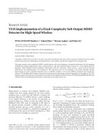
Figure 7 shows the compensation results for the weakly
nonlinear PA. The spectrum is measured after the down-
converter at 70 MHz centre frequency. For comparison, an
IBO was imposed on the uncompensated PA so that the in-
band power of the signal is leveled to that of the compensated
output. Results show that both the SCPWL PD and the secant
10 EURASIP Journal on Advances in Signal Processing
8078767472706866646260
f (MHz)
−60
−55
−50
−45
−40
−35

−30
−25
−20
−15
−10
P (dBm)
Sec. Volt. PD
SCPWL PD
PA w ith IB O
RBW
= 100 kHz, VBW = 10 kHz, ATT = 10 dB
Figure 7: Measured power spectra of a PA driven into a weakly
nonlinear region, comparison of a PA with IBO, secant Volterra PD,
and SCPWL PD.
Volterra PD were able to reduce the adjacent channel power
byapproximately12dBto15dB.
6.2. Results : strongly nonlinear PA
The SCPWL PD employed the same number of partitions,
that is, ten partitions in its model for compensation of
the strongly nonlinear PA. As for the secant Volterra PD, a
third-order polynomial was not sufficient for modeling the
stronger nonlinearity of the PA in this case. Instead, a fifth-
order power series was used to model the PA. In this test, the
spectrum analyzer was placed before the down-converter so
that a larger dynamic range can be observed (cf. Section 5.3).
The performance of the two PDs in the strongly nonlin-
ear case is shown in Figure 8. The secant Volterra PD achieves
an ACPR improvement of approximately 10 dB compared
to 12 dB improvement in the weakly nonlinear case. The
SCPWL PD outperforms the secant Volterra PD by approx-

imately 5 dB at the best case, resulting in an ACPR reduc-
tion of 15 dB. These results may be explained by the numer-
ical problem posed by the higher-order polynomial which
leads to inaccurate modeling of the stronger compressive be-
haviour. In this case, a piecewise linear function offers better
numerical properties for least-squares fitting.
Note that the PDs are ineffective outside of the 20 MHz
mask (marked by the dashed line) of the down-converter fil-
ter since the PDs are modeled from the bandlimited IO data
(i.e., IMD of fifth order and above cannot be compensated).
A relatively large IBO of 3 dB is necessary to level the in-
band power of the uncompensated PA to that of the compen-
sated ones.
7. FPGA IMPLEMENTATION AND REAL-TIME TEST
The real-time test was only performed on the iterative secant-
Volterra PD presented in Section 4.2.1. In this test mode, the
PD has to be first implemented on an FPGA. The implemen-
2.472.462.452.442.43
f (GHz)
−90
−85
−80
−75
−70
−65
−60
−55
−50
−45
−40

−35
−30
−25
−20
P (dBm)
Sec. Volt. PD
SCPWL PD
PA w ith IB O
= 3dB
RBW
= 100 kHz, VBW = 10 kHz, ATT = 10 dB
Figure 8: Measured power spectra of a PA driven into stronger non-
linear region, comparison of a PA with IBO, secant Volterra PD, and
SCPWL PD.
tation design is intended for demonstrating the implemen-
tation feasibility of the PD algorithm. Therefore, the com-
plexity is intentionally kept minimal, where only the AM/AM
characteristic of the PA is considered and is modeled using a
simple Taylor series with two coefficients.
In the following subsection, the implementation of the
iterative secant Volterra PD on the FPGA is described.
The resource optimisation for the FPGA implementation
and the fixed-point error analysis are performed before
the actual implementation on the FPGA and are discussed
in Section 7.2. The real-time test results are presented in
Section 7.3.
7.1. FPGA implementation of the secant Volterra PD
In the implementation design, the PA is modeled with a Tay-
lor series with first and third-order coefficients, given as
y[n]

= N

z[n]

=
θ
1
z[n]+θ
3
z[n]


z[n]


2
=

θ
1


z[n]


+ θ
3


z[n]



3

e
j arg (z[n])
,
(29)
where z[n]andy[n] are the input and output signal of
the PA, respectively. Only two real-valued model parameters
have to be estimated. It is clear that only third-order IMD
products can be captured with this PA model. The two pa-
rameters θ
1
and θ
3
, along with the intended linear gain g
are determined in the modeling part performed in the host
computer using a MATLAB program. These parameters are
needed as input to the FPGA.
Figure 9 illustrates the implementation of one iteration
of the secant Volterra PD algorithm in (20). This iterative
algorithm determines the output signal z[n] of the secant
Volterra PD. Note that in our implementation, the compu-
tation of
N(z[n]) is embedded in the the function T(z[n]).
The calculation requires the PA model parameters θ
1
and θ
3

,
the intended linear gain g, and the PD input signal u[n]ob-
tained from the modeling part. The required division in the
Ernst Aschbacher et al. 11
z
i
[n]
z
i−1
[n]
T

z
i−1
[n]

g · u[n]
+
−
T
÷
μ
i
+
−
·
+
−
z
i+1

[n]
T

z
i
[n]

z
i
[n]
g
·u[n]
z
I
[n − 1]
Figure 9: One iteration of the secant Volterra PD in detail.
algorithm is approximated with the Newton-Raphson itera-
tive procedure in order to keep the complexity as low as pos-
sible. The details of this division algorithm are given in the
appendix.
Figure 10 shows a graphical illustration of three iterations
of the PD algorithm implemented on the FPGA. The first
stage of the iteration starts with the two initial values z
0
[n] =
u[n]andz
−1
[n] = 0. The signal T(z
−1
[n]) =−g·u[n] since

N(z
−1
[n]) = 0. As the product g·u[n] is already determined
for each iteration, the initial value of
T(z
−1
[n]) = T(0) re-
quires effectively only a sign change. The following two stages
require the output signal and the function
T calculated from
their previous stages together with the product g
·u[n]. The
dashed line shows the feedback path which has to be imple-
mented if PA models with memory are considered (not done
in this implementation).
7.2. Fixed-point error analysis and
resource optimization
The FPGA used in our implementation is the XC2V1000 Xil-
inx Virtex-2 FPGA [43]. The Xilinx Vertex-2 provides a total
of forty multipliers which are implemented as hard macros.
2
These multipliers are optimized with respect to power con-
sumption and speed. Therefore, the device is suitable for de-
signs that require high clock rates, for example, algorithms
that process signals with large bandwidths. The maximum
bit width of these multipliers is 17 bits for unsigned values. In
this design, 17bits are used and the algorithm calculates the
sign separately. Before the PD algorithm is implemented on
the FPGA, the algorithm performed with fixed-point arith-
metic is simulated for fixed-point error analysis. The algo-

rithm needs to be optimized to obtain a balance between
the fixed-point error and the usage of the limited resources
(number of multipliers) provided by the FPGA.
At a glance from Figure 9, each iteration of the algo-
rithm in (20) requires nine multiplications, in which three
are needed for the implementation of the divider. However,
the product g
·u[n] in the function T
u
(z[n]) need only to be
2
Hard macros are unchangeable parts of programmable logic devices.
calculated in the initial stage as discussed in the last subsec-
tion. Therefore, after the initial stage, each iteration requires
eight multiplications. With the forty multipliers, a maximum
of four iterations can be accommodated.
Next, a Simulink model of the algorithm is implemented
with 17-bit operands and fixed-point arithmetic. The out-
put signal is compared to that generated by the same algo-
rithm executed with floating-point double-precision arith-
metic. With a multitone test signal, a third-order PA model
as in (29), and with three iterations of the secant algorithm
(20), the maximum relative error between the calculated sig-
nals in fixed-point precision and floating-point precision is
only 1.7% [45].
Finally, three iterations of the algorithm are implemented
in VHDL. A final VHDL simulation using ModelSim is per-
formed before implementation on the FPGA [45]. The simu-
lation provides a cycle-true and bit-true computation of the
predistorted signal. Figure 11 shows a measurement result on

the mildly nonlinear PA (cf. also Figure 7).ThePAwasex-
cited with predistorted signals calculated in Matlab and the
ModelSim simulation of the VHDL description. No perfor-
mance loss due to the fixed-point error can be observed from
the results.
7.2.1. FPGA resources
The developed PD design can be clocked with a maximum
clock frequency of 133 MHz. Approximately 50% of the
FPGA resources are used in the above implementation. The
remaining resources can be used for further enhancements,
for example, to support PA models with memory and/or PA
models with higher-order nonlinear terms.
7.3. Measurement results: real-time test
The secant Volterra PD which was implemented on the
FPGA as presented in Section 7.1 is tested in the real-time
mode. Each input sample is predistorted by the PD in real-
time. In this test, the PA is driven into a mildly nonlinear
region where significant third-order IMD is observed, but
fifth-order IMD is not significant.
The linearisation performance of the real-time secant
Volterra PD is compared to that of the offline secant Volterra
PD which was implemented in MATLAB (floating-point pre-
cision). Figure 12 shows the measurement results. No signifi-
cant performance loss can be observed in the real-time FPGA
implementation. Both the offline PD and real-time PD show
excellent linearisation performance—an ACPR suppression
of up to 15 dB is achieved.
The power loss in terms of required power back-off of
an uncompensated PA is demonstrated in Figure 13. The un-
compensatedPAisbackedoff to achieve an equal ACPR as

the compensated PA. A large IBO of 9 dB is necessary to re-
duce the ACI to the same level as achieved with the PD, lead-
ing to a significant in-band power loss of approximately 8 dB
compared to the in-band power of the linearised PA. This
proves the efficacy of the implemented PD design.
12 EURASIP Journal on Advances in Signal Processing
z
0
[n]
z
−1
[n]
T

z
−1
[n]

g · u[n]
Stage 1
z
1
[n]
z
0
[n]
T

z
0

[n]

Stage 2
z
2
[n]
z
1
[n]
T

z
1
[n]

Stage 3
q
−1
z
3
[n]
z
3
[n − 1]
Figure 10: Implemented three stages of the secant Volterra PD.
68676665646362
f (MHz)
−60
−55
−50

−45
−40
−35
−30
−25
−20
−15
−10
P (dBm)
No PD
PD-Matlab
PD-VHDL Sim.
RBW
= 100 kHz, VBW = 10 kHz, ATT = 10 dB
Figure 11: Measurement result on a mildly nonlinear PA with
and without PD: PD signal is calculated with floating-point preci-
sion (PD-MATLAB) and 17 bit fixed-point precision in a ModelSim
VHDL simulation (PD-VHDL Sim.).
8. CONCLUSIONS
We have proposed two digital predistorters (PD) that are
identified from measurement data of a broadband power
amplifier (PA). A measurement testbed was built for rapid
prototyping of the proposed PDs. The first PD is based
on the simplicial canonical piecewise linear (SCPWL) func-
tion which is capable only of compensating amplitude-
to-amplitude (AM/AM) distortion. The second PD uses a
Volterra model for modeling the nonlinearities, offering
the possibility to include memory effect compensation. The
SCPWL-PD is identified using a least-squares (LS)-based al-
gorithm. Due to the linear affine property of the function, the

computational complexity of the identification algorithm is
significantly reduced. As for the Volterra model PD, the pre-
inverse model is difficult to identify. Therefore, an iterative
method, namely, the secant method for root-finding, is used
for the identification of the Volterra model PD.
Two test modes were set up for the proposed PDs,
namely, the offline mode and the real-time mode. In the of-
fline test mode, the PDs are identified in a host computer us-
ing the identification algorithms programmed in MATLAB.
Then the excitation signal is predistorted in the host com-
puter and transferred to the memory for transmission again.
8078767472706866646260
f (MHz)
−95
−90
−85
−80
−75
−70
−65
−60
−55
−50
−45
−40
−35
−30
P (dBm)
Sec. Volt. PD, real-time
No PD, IBO 1 dB

Sec. Volt. PD, offline
RBW
= 100 kHz, VBW = 100 kHz, ATT = 10 dB
Figure 12: Measured output spectra at 70 MHz IF: comparison of
IBO and digital predistortion (secant Volterra PD) in offline and
real-time modes.
This mode allows quick assessment of the PD performance.
Both the SCPWL-PD and the Volterra PD are tested in this
mode. The performance of the two PDs were evaluated on a
mildly nonlinear PA and a strongly nonlinear PA. The mildly
nonlinear PA exhibits only third-order intermodulation dis-
tortion (IMD) while the latter exhibits mild fifth-order IMD.
It is observed that the SCPWL-PD performs better in the
strong nonlinear case. This result reflects the numerical in-
stability that polynomial models pose when modeling strong
nonlinearity. Modelling inaccuracy leads to PD performance
loss.
In the real-time test mode, the Volterra model PD identi-
fied using the secant method was implemented on a fixed-
point arithmetic FPGA Xilinx Virtex-2 XC2V1000. In or-
der to evaluate the implementation feasibility of the itera-
tive method, the complexity of the model is kept minimal.
A memoryless third-order power series was used and three
iterations of the secant method were implemented on the
FPGA. Only 50% of the FPGA resources were used in this
implementation. Besides implementation feasibility and per-
formance evaluation, this test mode also allows to compare
the performance of fixed-point arithmetic and floating-point
arithmetic for PD implementation. No significant perfor-
mance loss in terms of adjacent channel power ratio (ACPR)

is observed in the fixed-point arithmetic implementation as
Ernst Aschbacher et al. 13
8078767472706866646260
f (MHz)
−100
−95
−90
−85
−80
−75
−70
−65
−60
−55
−50
−45
−40
−35
−30
P (dBm)
Sec. Volt. PD, real-time
No PD, 9 dB IBO
No PD, 1 dB IBO
RBW
= 100 kHz, VBW = 100 kHz, ATT = 10 dB
Figure 13: Measured output spectra at 70 MHz IF: comparison of
IBO and digital predistortion with the secant Volterra PD (real-
time) for achieving equal out-of-band distortions.
Table 1: Starting values for the Newton-Raphson method applied
for performing a division 1/d, d being represented by four bits and

interpreted as a fractional number.
kI
k
Exact value, x = 1/d Starting value, x
0
= 2
k−1
1

5
8
,1

8
5
,1

2
0
= 1
2

3
8
,
4
8

8
3

,2

2
1
= 2
3
2
8
42
2
= 4
4
1
8
82
3
= 8
compared to the floating-point arithmetic implementation
(MATLAB program).
Overall, both the PDs show good linearisation perfor-
mance. In compensating the mildly nonlinear PA, both the
PDs were able to reduce the ACPR by approximately 15 dB
with the Volterra PD performing slightly better. However,
when the PA is driven to a stronger nonlinear region, the
performance of the Volterra model PD degraded by approx-
imately 5 dB leading to an ACPR reduction of 10 dB while
the performance of the SCPWL-PD remains the same. We
have also shown that in order for the uncompensated PA to
match the ACPR level of the compensated PA output, an IBO
of 9 dB is required leading to an in-band power loss of 8 dB

in the transmitted signal. This in turn indicates the power
efficiency to gain a PD can provide for systems that require
linear transmission.
APPENDIX
A. APPROXIMATION OF THE DIVISION
The FPGA provides optimised hardware multipliers but does
not provide optimised hardware dividers. The XILINX Logi-
Core library provides an IP-core for a divider implementa-
tion [46] but it proves to be too costly in terms of resources.
Therefore, an alternative method, based on the Newton-
Raphson root-finding algorithm, is used [45]. If a division
r
=
n
d
= n·
1
d
= n·x (A.1)
has to be performed, the task is to calculate x
= 1/d and
multiply the result with the numerator n. Rearranging terms
gives
d
−
1
x
= f (x) = 0, (A.2)
which can be solved with the Newton-Raphson method
x

i+1
= x
i
−
f (x
i
)
f

(x
i
)
= x
i
(2 −dx
i
), i ≥ 0, x
0
given. (A.3)
The convergence rate of the Newton-Raphson algorithm is
quadratic, therefore, it can be expected that few iterations are
sufficient. Further, the starting value x
0
can be chosen freely
and, thus, a list of optimised starting values can be produced.
Based on the value of d, the optimal value x
0
can be chosen. If
x
0

is further chosen to be a power of two, the multiplications
with x
0
reduce to cheap shift-operations. In this way, the first
iteration x
1
is computed without a multiplication.
The range of the possible values for fractional numbers,
3
which are used in this design, is divided into N − 1 inter-
vals I
k
≡ [2
−k
+ Δ;2
−(k−1)
], k = 1, 2, , N − 1, Δ being the
resolution Δ
= 2
−(N−1)
. The starting-value x
0
for each inter-
val is then chosen to be x
0
= 2
k−1
if d ∈ I
k
, thus, at the up-

per limit of the interval, the correct result is obtained with
the starting value. Ta ble 1 shows an example list of starting
values, assuming that the number d is given by a fractional
1.3 two-complement representation and only positive values,
ranging from 1 to Δ are taken into account. The resolution
(or numerical value of the least significant bit) in this case is
Δ
= 2
−3
= 1/8.
It can be shown that with these starting-values the
Newton-Raphson algorithm is guaranteed to converge [48].
An error analysis [48] shows that after the second iteration,
the relative error ε
2
= (x
2
− x)/x is only 6.25%. The arith-
metic cost for the division, if two iterations are performed,
is only two multiplications (the multiplications with the ini-
tial value in the first iteration are shift operations) and three
subtractions. With the multiplication of the numerator, three
multiplications in total are necessary.
REFERENCES
[1] R.D.J.vanNeeandR.Prasad,OFDM for Wireless Multimedia
Communications, Artech House, London, UK, 2000.
[2]A.R.S.Bahai,B.R.Saltzberg,andM.Ergen,Multi-Carr ier
Digital Communications: Theory and Applications of OFDM,
Springer, New York, NY, USA, 2nd edition, 2004.
3

Anumberx can be represented with N bits in I.Q-format, I = 1, Q =
N −1as[47] x =−b
N−1
+

N−1
k
=1
b
N−1−k
2
−k
, b
N−1−k
∈{0,1}and −1 ≤
x ≤ 1 −2
−N+1
.TheresolutionisΔ= 2
−N+1
.IfN = 4, Δ= 2
−3
= 0, 125.
14 EURASIP Journal on Advances in Signal Processing
[3] “3rd Generation Partnership Project,” .
[4] P. B. Kenington, High Linearity RF Amplifier Design,Artech
House, London, UK, 2000.
[5] T. Nojima, T. Murase, and N. Imai, “The design of a predis-
tortion linearization circuit for high-level modulation radio
systems,” in Proceedings of IEEE Global Telecommunications
Conference (GLOBECOM ’85), vol. 3, pp. 1466–1471, New Or-

leans, La, USA, December 1985.
[6] T. Nojima and T. Konno, “Cuber predistortion linearizer for
relay equipment in 800 MHz band land mobile telephone sys-
tem,” IEEE Transactions on Vehicular Technology, vol. 34, no. 4,
pp. 169–177, 1985.
[7] S. P. Stapleton and F. C. Costescu, “An adaptive predistorter
for a power amplifier based on adjacent channel emissions,”
IEEE Transactions on Vehicular Technology,vol.41,no.1,pp.
49–56, 1992.
[8] A. Bateman, D. M. Haines, and R. J. Wilkinson, “Linear
transceiver architectures,” in Proceedings of the 38th IEEE
Vehicular Technology Conference (VTC ’88), pp. 478–484,
Philadelphia, Pa, USA, June 1988.
[9] M. Faulkner and M. Johansson, “Adaptive linearization using
predistortion-experimental results,” IEEE Transactions on Ve-
hicular Technology, vol. 43, no. 2, pp. 323–332, 1994.
[10] J. K. Cavers, “A linearizing predistorter with fast adaptation,”
in Proceedings of the 40th IEEE Vehicular Technology Conference
(VTC ’90), pp. 41–47, Orlando, Fla, USA, May 1990.
[11] E. Changsoo and E. J. Powers, “A new volterra predistorter
based on the indirect learning architecture,” IEEE Transactions
on Signal Processing, vol. 45, no. 1, pp. 223–227, 1997.
[12] A. Saleh, “Frequency-independent and frequency-dependent
nonlinear models of TWT amplifiers,” IEEE Transactions on
Communications, vol. 29, no. 11, pp. 1715–1720, 1981.
[13] Y. Nagata, “Linear amplification technique for digital mobile
communications,” in Proceedings of the 39th IEEE Vehicular
Technology Conference (VTC ’89), pp. 159–164, San Francisco,
Calif, USA, May 1989.
[14] E. G. Jeckeln, F. M. Ghannouchi, and M. A. Sawan, “An L band

adaptive digital predistorter for power amplifiers using direct
I-Q modem,” in Proceedings of IEEE MTT-S International Mi-
crowave Symposium Digest (MWSYM ’98), vol. 2, pp. 719–722,
Baltimore, Md, USA, June 1998.
[15] S. Boumaiza, J. Li, and F. M. Ghannouchi, “Implementation
of an adaptive digital/RF predistorter using direct LUT syn-
thesis,” in Proceedings of IEEE MTT-S International Microwave
Symposium (IMS ’04), vol. 2, pp. 681–684, Fort Worth, Tex,
USA, June 2004.
[16] H. Ben Nasr, S. Boumaiza, M. Helaoui, A. Ghazel, and F. M.
Ghannouchi, “On the critical issues of DSP/FPGA mixed digi-
tal predistorter implementation,” in Proceedings of Asia-Pacific
Conference on Microwave Conference (APMC ’05), vol. 5, p. 4,
Suzhou, China, December 2005.
[17] L. Ding, H. Qian, N. Chen, and G. T. Zhou, “A memory poly-
nomial predistorter implemented using TMS320C67xx,” in
Proceedings of Texas Instruments Developer Conference,pp.1–
7, Houston, Tex, USA, February 2004.
[18] N. Chen, G. T. Zhou, and H. Qian, “Power efficiency im-
provements through peak-to-average power ratio reduction
and power amplifier linearization,” EURASIP Journal on Ad-
vances in Signal Processing, vol. 2007, Article ID 20463, 7 pages,
2007.
[19] L. Ding, Z. Ma, D. R. Morgan, M. Zierdt, and J. Pasta-
lan, “A least-squares/Newton method for digital predistortion
of wideband signals,” IEEE Transactions on Communications,
vol. 54, no. 5, pp. 833–840, 2006.
[20] “Mini-Circuits ZVE-8G Amplifier,” icircuits
.com/pdfs/ZVE-8G.pdf.
[21] 3rd Generation Partnership Project, “Technical Specifica-

tion Group Radio Access Network; Base Station (BS) radio
transmission and reception (FDD) (Release 6), TS 25.104,”
.
[22] F. H. Raab, P. Asbeck, S. Cripps, et al., “Power amplifiers and
transmitters for RF and microwave,” IEEE Transactions on Mi-
crowave Theory and Techniques, vol. 50, no. 3, pp. 814–826,
2002.
[23] L. O. Chua and S. M. Kang, “Section-wise piecewise-linear
functions: canonical representation, properties, and applica-
tions,” Proceedings of the IEEE, vol. 65, no. 6, pp. 915–929,
1977.
[24] P. Julian, A. Desages, and O. Agamennoni, “High-level canon-
ical piecewise linear representation using a simplicial parti-
tion,” IEEE Transactions on Circuits and Systems, vol. 46, no. 4,
pp. 463–480, 1999.
[25] M J. Chien and E. Kuh, “Solving nonlinear resistive networks
using piecewise-linear analysis and simplicial subdivision,”
IEEE Transactions on Circuits and Systems,vol.24,no.6,pp.
305–317, 1977.
[26] C. Guzelis and I. C. Goknar, “A canonical representation for
piecewise-affine maps and its applications to circuit analysis,”
IEEE Transactions on Circuits and Systems, vol. 38, no. 11, pp.
1342–1354, 1991.
[27] B. Fronberg, A Practical Guide to Pseudospectral Methods,
Cambridge University Press, New York, NY, USA, 1998.
[28] M. Y. Cheong, S. Werner, J. Couss
´
eau, J. L. Figueroa, and T. I.
Laakso, “Predistorter design employing parallel piecewise lin-
ear structure and inverse coordinate mapping for broadband

communications,” in Proceedings of the 14th European Signal
Processing Conference (EUSIPCO ’06), pp. 1–5, Florence, Italy,
September 2006.
[29] N. Wiener, Nonlinear Problems in Random Theory,JohnWiley
& Sons, New York, NY, USA, 1958.
[30] M. Schetzen, The Volterra and Wiener Theories of Nonlinear
Systems, John Wiley & Sons, New York, NY, USA, 1980.
[31] S. Boyd and L. O. Chua, “Fading memory and the problem of
approximating nonlinear operators with volterra series,” IEEE
Transactions on Circuits and Systems, vol. 32, no. 11, pp. 1150–
1161, 1985.
[32] D. Hummels and R. Gitchell, “Equivalent low-pass represen-
tations for bandpass volterra systems,” IEEE Transactions on
Communications, vol. 28, no. 1, pp. 140–142, 1980.
[33] M. Y. Cheong, E. Aschbacher, P. Brunmayr, M. Rupp, and
T. I. Laakso, “Comparison and experimental verification of
two low-complexity digital predistortion methods,” in Pro-
ceedings of the 39th Asilomar Conference on Signals, Systems and
Computers, pp. 432–436, Pacific Grove, Calif, USA, October-
November 2005.
[34] M. Schetzen, “Theory of pth-order inverses of nonlinear sys-
tems,” IEEE Transactions on Circuits and Systems,vol.23,no.5,
pp. 285–291, 1976.
[35] D. G. Luenberger, Optimization by Vector Space Methods,John
Wiley & Sons, New York, NY, USA, 1968.
[36] A. M. Ostrowski, Solution of Equations and Systems of Equa-
tions, Academic Press, New York, NY, USA, 1960.
[37] R. D. Nowak and B. D. V. Veen, “Volterra filter equalization: a
fixed point approach,” IEEE Transactions on Signal Processing,
vol. 45, no. 2, pp. 377–388, 1997.

[38] Advanced Design System (ADS), “Agilent Technologies,”
/>main.html.
Ernst Aschbacher et al. 15
[39] Sundance SMT310Q PCI Carrier Board, dance
.com/docs/SMT310Q%20User%20Manual.pdf.
[40] Sundance SMT351-G module, />docs/SMT351%20User%20Manual.pdf.
[41] Sundance SMT370-AC module, />docs/SMT370%20User%20Manual.pdf.
[42] Analog Devices D/A converter AD9777, log
.com/UploadedFiles/Data
Sheets/3229938536490156500AD-
9777
b.pdf.
[43] XILINX Virtex-II Platform FPGA, />partinfo/ds031.pdf.
[44] Sundance SMT365 module, />smt365%20user%20manual.pdf.
[45] P. Brunmayr, “Implementation of a nonlinear digital pre-
distortion algorithm,” M.S. thesis, Vienna University of Tech-
nology, Institute of Communications and Radio-Frequency
Engineering, Vienna, Austria, 2005,
.at/files/pub-et
10048.pdf.
[46] XILINX IP Core Pipelined Divider, />bvdocs/ipcenter/data
sheet/sdivider.pdf.
[47] G. Doblinger, Signalprozessoren—Architekturen, Algorithme n,
Anwendungen, J. Schlembach Fachverlag, Weil der Stadt, Ger-
many, 2000.
[48] E. Aschbacher, “Digital pre-distortion of microwave power
amplifiers,” Ph.D. dissertation, Vienna University of Tech-
nology, Institute of Communications and Radio-Frequency
Engineering, Austria, 2005, />pub-et
11772.pdf.