Báo cáo hóa học: " Research Article A TOA-AOA-Based NLOS Error Mitigation Method for Location Estimatio" docx

Hindawi Publishing Corporation
EURASIP Journal on Advances in Signal Processing
Volume 2008, Article ID 682528, 14 pages
doi:10.1155/2008/682528
Research Article
A TOA-AOA-Based NLOS Error Mitigation Method for
Location Estimation
Hong Tang,
1
Yongwan Park,
1
and Tianshuang Qiu
2
1
Mobile Communication Laboratory, Yeungnam University, kyongsan, kyongbuk 712-749, South Korea
2
School of Electronic and Information Engineering, Dalian University of Technology, Liaoning 116024, China
Correspondence should be addressed to Yongwan Park,
Received 28 February 2007; Revised 21 July 2007; Accepted 31 October 2007
Recommended by Sinan Gezici
This paper proposes a geometric method to locate a mobile station (MS) in a mobile cellular network when both the range and
angle measurements are corrupted by non-line-of-sight (NLOS) errors. The MS location is restricted to an enclosed region by
geometric constraints from the temporal-spatial characteristics of the radio propagation channel. A closed-form equation of the
MS position, time of arrival (TOA), angle of arrival (AOA), and angle spread is provided. The solution space of the equation is
very large because the angle spreads are random variables in nature. A constrained objective function is constructed to further
limit the MS position. A Lagrange multiplier-based solution and a numerical solution are proposed to resolve the MS position.
The estimation quality of the estimator in term of “biased” or “unbiased” is discussed. The scale factors, which may be used
to evaluate NLOS propagation level, can be estimated by the proposed method. AOA seen at base stations may be corrected to
some degree. The performance comparisons among the proposed method and other hybrid location methods are investigated on
different NLOS error models and with two scenarios of cell layout. It is found that the proposed method can deal with NLOS error
effectively, and it is attractive for location estimation in cellular networks.

Copyright © 2008 Hong Tang et al. This is an open access article distributed under the Creative Commons Attribution License,
which permits unrestricted use, distribution, and reproduction in any medium, provided the original work is properly cited.
1. INTRODUCTION
Wireless location for a mobile station (MS) in a cellular net-
work has gained tremendous attention in the last decade
due to support from the Federal Communication Commis-
sion (FCC) and wide range of potential applications using
location-based information. Accurate positioning is already
considered as one of the essential features of third generation
(3G) wireless systems in winning a wide acceptance. Most
location techniques depend on the measurements of time of
arrival (TOA), received signal strength (RSS), time difference
of arrival (TDOA), and/or angle of arrival (AOA) [1–5]. For
TOA location methods, the TOA measurement provides a
circle centered at the base station (BS) on which the MS must
lie. The MS location estimate is determined by the intersec-
tion of circles; at least three BSs are involved in the location
process to resolve ambiguities arising from multiple cross-
ing of the positioning lines. The RSS-based location has the
same trilateration concept if the propagation path losses are
transformed into distances. For TDOA location methods, the
distance differences of the MS to at least three BSs are mea-
sured. Each TDOA measurement provides a hyperbolic lo-
cus on which the MS must lie and the position estimate is
determined by the intersection of two or more hyperbolas.
For AOA location methods, the angle of arrival of the MS to
the BS is measured by multielement antenna array or multi-
beamforming antenna. A line from the MS to the BS can be
drawn according to each AOA measurement and the position
of the MS is calculated from the intersection of at least two

lines. High accuracy can be derived from these methods with
the assumption of line-of-sight (LOS) propagation. However,
location errors will inevitably increase greatly as the assump-
tion is violated by NLOS.
NLOS can cause different range error in different prop-
agation environments, from dozen of meters to thousands
of meters [6]. In open area there are almost no obstacles.
The signal travels in LOS. However, in mountains, urban
environments, or bad urban environments, the signal may
transmit in reflection, diffraction; and it takes longer for the
signal to arrive at the receiver. As a result the range error
caused by NLOS is always a positive number. In [7], LOS
was reconstructed using the statistics of the measurement
2 EURASIP Journal on Advances in Signal Processing
data. Mathematical programming techniques were adopted
in [5, 8–10] to evaluate the NLOS propagation effect. No
prior knowledge was required in [8–10], but the variance
of measurement noise was required in [5]. A method to de-
termine and identify the number of line-of-sight BSs based
on a residual test was proposed in [11]. In [12], a geomet-
ric location method was proposed. It can suppress NLOS er-
ror to some degree. Scattering-model-based methods were
proposed to classify propagation environments via moment
matching, expectation maximization, and Bayesian estima-
tion in [13]. The bias of time measures in NLOS environment
was tracked with Kalman filter in [14], and the evaluation of
the approach was carried out in real scenarios.
From the basic principle of the time-based location
methods [8–12], we know that they are valid only when at
least three BSs can support the location process. However,

this requirement may not always be met at all times because
of the hearability limitation of an MS, that is, the ability of
a mobile to listen to a BS. The field trials in [6]conducted
in a GSM network showed that over 92% of the time in ur-
ban environments and 71% of the time in rural environ-
ments, three or more BSs can be received by the MS. How-
ever, for two or more BSs, the corresponding percentages
are 98% and 95%, for each environment. This means that
about 6% of the time in urban environments and 24% of
the time in rural environments only two BSs can support an
MS.Orinsomecases,moreBSscansupportanMS,butonly
two BSs have high reliability for location purpose. Or some-
where, the BSs are sparse and only two BSs may be avail-
able. Thus the time-based location methods will suffer from
ambiguity.
Hybrid location methods by combining time measure-
ment and angle measurement can reduce the number of re-
ceiving BSs and improve the coverage of location-based ser-
vice in cellular network simultaneously. The reference [4, 15–
19] proposed hybrid location methods which can be applied
when only two BSs are involved. The AOA data fusion in
[4] combined TOAs and AOAs into a group of linear equa-
tions. In [15], by taking advantage of two TOAs seen at the
two BSs and AOA seen at home BS, the author proposed
geometry-constrained location estimation (GLE) method to
estimate the MS position. In [16], hybrid lines of position
(HLOP) method were proposed, which combined the lin-
ear lines of position (LOP) generated by differencing pairs
of squared range estimates and the linear LOP given by the
AOA. In [17], two equations were built. One equation was

built from TDOA and the other was built from AOA. Be-
cause closed form solution of the two equations is quit com-
plex, a new coordinate system was constructed to simplify
the two equations. Reference [18]focusedonAOA-basedlo-
cation method which selected the two most reliable AOAs
among the whole set of AOA measurements. The TOA-based
historical data was used in [19] to resolve location ambi-
guity and Kalman filter was adopted to track trajectory. We
note that these methods [15–17] only take advantage of the
AOA seen at home BS. Other hybrid location methods can be
found in [20–22]. And all of them [4, 15–22] seldom consider
the temporal-spatial characteristics of the radio propagation
channel.
This paper proposes an NLOS mitigation method mo-
tivated by the temporal-spatial characteristics of the radio
channel. The geometric explanation of the method is pre-
sented in Section 2, including the temporal-spatial chan-
nel models, TOA, and AOA measurements. The mathematic
model is given in Section 3, including the constraints de-
rived from TOAs, AOAs, and angle spreads, and the construc-
tion of objective function. The solution and analysis to the
model are presented in Section 4
, including the Lagrange-
based solution and estimation quality in terms of “biased”
or “unbiased.” The case of three BSs is discussed in Section 5.
And the numerical solution is presented in Section 6.Com-
puter simulation results are presented in Section 7 to show
the performance, and remarks and conclusions are provided
in Section 8.
2. GEOMETRIC EXPLANATION TO

THE PROPOSED METHOD
2.1. The temporal-spatial channel models of
the propagation channel
The temporal-spatial channel model can provide both delay
spread and angle spread statistics of the channel. The angle
spread is dependent on the wireless propagation environ-
ment. In a macrocell, the antenna height at the MS is low.
The scatters surrounding the MS are about the same height
or are higher than the MS. This results in the MS-received
signal arriving from all directions after bouncing from sur-
rounding scatters. AOA seen at the MS can be modeled as a
random variable uniformly distributed over [0,2π]. On the
other hand, the antenna height at the BS is much higher than
the surrounding scatters. The BS may not receive multipath
reflections from locations near the BS. The received signal
at the BS mainly comes from the scattering process in the
vicinity of the mobile. AOA seen at the BS is restricted to
a small angular region. And it is no longer uniformly dis-
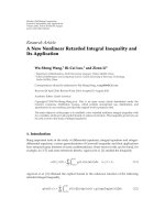
tributed over [0, 2π]. A circular mode was proposed in [23]
to describe the joint TOA/AOA probability density function
(pdf) as seen in Figure 1, where the scatters are assumed to
be uniformly distributed in a circle and an MS is the cen-
ter of the circle. This is the so-called circular disk of scatters
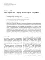
model (CDSM). For example, when the distance from MS
to BS is 1000 meters and the scattering radius is 200 meters,
the marginal TOA pdf and the marginal AOA pdf are shown
in Figures 2(a) and 2(b), respectively. It can be found that
the absolute angle spread is within 11 degrees and the ex-
cess delay is within 1.4 microseconds. In a microcell, both
the antenna heights at BSs and MSs are low. The scatters are

near the BS and the MS. An elliptical model is used to model
this propagation environment. The scatters are assumed to
be uniform distributed in an ellipse where the BS and the MS
are the two foci. AOA seen at the BS has a larger angle spread.
But it is also found that the joint AOA/TOA components seen
at the BS are concentrated near line-of-sight [23]. The mea-
surement campaigns reported in [24] are consistent with the
above CDSM. It is suggested that AOA seen at the BS in a
macrocell is like a Gaussian distribution with typical stan-
dard deviation of angle spreads approximately 6 degrees, and
Hong Tang et al. 3
D
Base
station
Mobile
Scattering region
+
+
+
+
+
+
+
+
Figure 1: Circular scatter geometry for a macrocell.
the delay spread can be described by an exponential distribu-
tion. Further discussion about angle spread can be found in
[25] and the references therein. The temporal-spatial charac-
teristics of the propagation channel derived in [24]tendto
be consistent with the results in [23, 25].

The other models are used to study delay spread is the
ring of scatters model (ROSM) [13, 26] and the distance-
dependent model (DDM) [10, 27]. The ROSM is also a classi-
cal model to describe macrocellular environments where the
scatters are uniformly distributed on a ring which is centered
about the MS. In the DDM, the delay spread is taken to be
proportional to the LOS distance. The paper [27]citedmea-
surement results from Motorola and Ericsson that report a
relationship between the mean excess delay τ
m
and the root-
mean-square (rms) delay spread τ
rms
of the form τ
m
= kτ
rms
,
where k is proportionality constant. The observation and re-
sults from [28] also suggested that NLOS errors may increase
with distance.
2.2. The measurements on TOA and AOA in
cellular network
Theschemetoperformrangemeasurementmaybediffer-
ent in different systems. In the TDMA system, the time delay
between the MS and the serving BS must be known to avoid
overlapping time slots. This is called timing advance (TA).
For example, TA is available in GSM and TD-SCDMA. TA
can be used to approximate the distance between the serv-
ing BS and the MS. In the CDMA system, time delay can be

estimated by coarse timing acquisition with a sliding corre-
lator or fine timing acquisition with a delay loop lock (DLL).
The later is better suited for a location system, as illustrated
in [29].Roundtripdelay(RTD)isageneralmethodtode-
termine the distance between the transmitter and receiver,
which needs a time stamp when the signal is transmitted and
a time stamp when the signal is received. The range is ap-
proximated by the time difference of the two time stamps.
So, it is technically easy to approximate the distance between
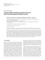
the MS and the serving BS. In this paper, it is firstly assumed
that only two BSs can support the MS, that is, BS1 and BS2 as
shown in Figure 3. BS1 is the serving BS. In order to get the
distance to the other BS, the so-called “force handover” could
be a good choice [6]. When the locating is to be done, the net-
work will force the MS to make a handover attempt from the
serving BS to the other BS. Usually the other BS is the clos-
est neighbor BS. The neighbor BS will measure the TA argu-
ment in the TDMA system or the time delay in the CDMA
system (or other techniques are taken to perform range mea-
surement) and then reject the handover request. The range
measurement r
i
between an MS to the BSi is expressed as
r
i
= c·

t
d,i
+ t

e,i

, i = 1, 2, (1)
where c is the speed of light, t
d,i
is the LOS path delay to
the BSi,andt
e,i
is the excess delay caused by NLOS. The two
TOAmeasurementsprovidetwocircles.Becauset
e,i
is always
a positive number, the MS position must be in an area over-
lapped by the two circles, as shown in Figure 3.
With the introduction of smart antenna array into wire-
less communication networks, the AOA of each MS can be
estimated. Usually the subspace-based AOA estimation algo-
rithms have good accuracy and resolution, such as the MU-
SIC [30] and ESPRIT algorithms. Multibeam antennas re-
ported in [31]werealsousedtoestimateAOAofanMS.
For example, in TD-SCDMA technical specification [32], the
precision of AOA for location purposes was required to be
15 degrees. In the NLOS environment the transmitted signal
could only reach the receiver through reflected, diffracted, or
scattered paths. Thus the AOA observed at the BS is not the
exact LOS path AOA. The AOA measurement mainly consists
two parts, which can be expressed as
θ
i
= θ

d,i
+ φ
i
, i = 1, 2, (2)
where θ
d,i
is the LOS path AOA and φ
i
is the angle spread
caused by NLOS propagation, which can be accurately de-
scribed by a Gaussian random variable in a macrocell or out-
door environment. The standard deviation of the Gaussian
distribution can be predicted by theoretical model or cal-
culated from experimental data. Therefore, it is possible to
know the angular bounds from the statistics of the AOA dis-
tribution of a given NLOS environment. That is, the LOS
path AOA must be in an interval with a certain high con-
fidence level. It is assumed that θ
min,i
and θ
max,i
are corre-
sponding upper and lower bounds. Then the following in-
equality holds (or holds with a sufficiently high confidence
level):
θ
min,i
≤ θ
d,i
≤ θ

max,i
, i = 1, 2. (3)
For example, if the angle spread seen at BSi is modeled as
a Gaussian distribution N(0, σ
2
), θ
d,i
must be in the inter-
val [θ
i
− 2σ, θ
i
+2σ] with confidence level 95.4%, where σ
is the standard deviation. Therefore, the MS position is fur-
ther constrained to a small enclosed region overlapped by the
two circles and the angular bounds, as illustrated in Figure 3,
that is, the estimated MS position must satisfy the following
restrictions:
r
d,i
≤ r
i
, i = 1, 2,
θ
min,i
≤

θ
d,i
≤ θ

max,i
, i = 1, 2,
(4)
where
r
d,i
and

θ
d,i
are the estimates of LOS range and LOS
AOA between the BSi and the MS, respectively.
TOAandAOAinamicrocellcanbedescribedbyanel-
liptical model [23], where the AOA measurement tends to
4 EURASIP Journal on Advances in Signal Processing
0
0.002
0.004
0.006
0.008
0.01
0.012
0.014
Probability density
00.511.5
TOA spread (μs)
(a)
0.2
0.4
0.6

0.8
1
1.2
1.4
1.6
1.8
2
×10
−3
Probability density
−15 −10 −50 51015
AOA spread (deg)
(b)
Figure 2: The temporal-spatial characteristics of the propagation channel in a macrocell where the distance from the MS to the BS is 1000
meters and the scatter radius is 200 meters. (a) The marginal TOA pdf and (b) the marginal AOA pdf.
W
X
Y
V
U
BS1
BS2
MS
Figure 3: Geometry constraints from the temporal-spatial channel
show that the MS lies in the overlapped region.
have large spread over [0, 2π]. Fortunately, the cell coverage
is small in a microcell environment and more than two BSs
may be received. The time-based location methods will not
suffer from ambiguity.
3. MATHEMATICAL MODEL TO THE MS

POSITION ESTIMATION
3.1. Constraints from TOA measurements
The location process is considered in a two-dimensional
(2D) space and two BSs are involved. Let (x
0
, y
0
) be the MS
position to be determined and let (x
i
, y
i
) be the coordinate
of BSi,wherei
= 1, 2. r
i
is the range measurement. In the
NLOS propagation environment, r
i
is always larger than the
LOS range. The following inequality must hold:


x
0
−x
i

2
+


y
0
− y
i

2
≤ r
i
, i = 1, 2. (5)
In order to change the inequality (5) into equality, let the
variable α
i
be the scale factor of r
i
. α
i
must be constrained to
η
i
≤ α
i
≤ 1, (6)
where η
1
= (R −r
2
)/r
1
and η

2
= (R −r
1
)/r
2
. R is the distance
between the two BSs. We get


x
0
−x
i

2
+

y
0
− y
i

2
= α
i
r
i
, i = 1, 2. (7)
Define the 2D function d
i

(x, y) which expresses the distance
between the position (x, y) and the BSi:
d
i
(x, y) =


x − x
i

2
+

y − y
i

2
, i = 1, 2. (8)
If (x
s
, y
s
) is an approximation position of the true MS posi-
tion, the function d
i
(x, y) can be expanded in Taylor’s series:
d
i
(x, y) ≈ d
i


x
s
, y
s

+
∂d
i
(x, y)
∂x




x=x
s
y=y
s

x − x
s

+
∂d
i
(x, y)
∂y





x=x
s
y=y
s

y−y
s

.
(9)
Hong Tang et al. 5
In (9), only the terms of zero-order and first-order are kept.
Let ω
0
= [x
0
, y
0
]
T
and C(ω
0
) = [d
1
(ω
0
), d
2

(ω
0
)]
T
be the
distance vectors. According to (9), C(ω
0
)canbewrittenas
C

ω
0

≈ C

ω
s

+ H

ω
s

ω
0
−ω
s

(10)
H(ω

s
) is the gradient matrix
H

ω
s

=
⎡
⎢
⎢
⎢
⎢
⎣
x
s
−x
1
d
1
(ω
s
)
y
s
− y
1
d
1
(ω

s
)
x
s
−x
2
d
2
(ω
s
)
y
s
− y
2
d
2
(ω
s
)
⎤
⎥
⎥
⎥
⎥
⎦
. (11)
From (7)and(10), an equality that describes a linear range
model incorporating NLOS errors can be expressed as
H


ω
s

·ω
0
−L = H

ω
s

·ω
s
−C

ω
s

, (12)
where L
= [α
1
r
1
, α
2
r
2
]
T

is the corrected distance vector.
Equation (12) can be rearranged as
⎡
⎢
⎢
⎢
⎢
⎢
⎣
x
s
−x
1
d
1

ω
s

y
s
− y
1
d
1

ω
s

−

r
1
0
x
s
−x
2
d
2

ω
s

y
s
− y
2
d
2

ω
s

0 −r
2
⎤
⎥
⎥
⎥
⎥

⎥
⎦
⎡
⎢
⎢
⎢
⎣
x
0
y
0
α
1
α
2
⎤
⎥
⎥
⎥
⎦
=
H

ω
s

·ω
s
−C


ω
s

.
(13)
3.2. Constraints from AOA measurements
It is assumed that the two BSs and the MS are in a coor-
dinate system as shown in Figure 4. AOA seen at BS1 is θ
1
and the corresponding angle spread is φ
1
. AOA seen at BS2
is θ
2
and the corresponding angle spread is φ
2
. From the ge-
ometry relationships shown in Figure 4, it can be found that
the equation CB
= CA − BA holds where CB = r
d,1
sin(φ
1
),
CA
= x
0
sin(θ
1
), and BA = y

0
cos(θ
1
). We obtain the follow-
ing equation:
x
0
sin

θ
1

− y
0
cos

θ
1

= r
d,1
sin

φ
1

, (14)
where r
d,1
is the LOS distance between the MS and BS1. It can

be rewritten as r
d,1
= α
1
r
1
. Therefore, (14) can be modified
to
x
0
sin

θ
1

−
y
0
cos

θ
1

−
α
1
r
1
sin


φ
1

=
0. (15)
Similarly, the equation ED
= EA − DA holds, where EA =
(x
2
− x
0
)sin(π − θ
2
), DA = y
0
cos(π − θ
2
), and ED =
α
2
r
2
sin(φ
2
). The following equation holds:
x
0
sin

θ

2

−
y
0
cos

θ
2

−
α
2
r
2
sin

φ
2

=
x
2
sin

θ
2

. (16)
Combining (15)and(16)gives


sin

θ
1

−
cos

θ
1

−
r
1
sin

φ
1

0
sin

θ
2

−
cos

θ

2

0 −r
2
sin

φ
2


⎡
⎢
⎢
⎢
⎣
x
0
y
0
α
1
α
2
⎤
⎥
⎥
⎥
⎦
=


0
x
2
sin

θ
2


.
(17)
BS1 BS2
MS
C
B
A
D
E
φ
1
φ
2
θ
1
θ
2
y
0
r
d,1

r
d,2
x
0
x
2
R − x
0
Figure 4: Constraints from AOA measurements.
3.3. MS position estimation
Combining (13)and(17) into a single matrix-vector form
gives
A
4×4
ω

4×1
= b
4×1
, (18)
where
A
4×4
=
⎡
⎢
⎢
⎢
⎢
⎢

⎢
⎢
⎢
⎢
⎢
⎣
x
s
−x
1
d
1

ω
s

y
s
− y
1
d
1

ω
s

−
r
1
0

x
s
−x
2
d
2

ω
s

y
s
− y
2
d
2

ω
s

0 −r
2
sin

θ
1

−cos

θ

1

−r
1
sin

φ
1

0
sin

θ
2

−
cos

θ
2

0 −r
2
sin

φ
2

⎤
⎥

⎥
⎥
⎥
⎥
⎥
⎥
⎥
⎥
⎥
⎦
,
ω

4×1
=

x
0
y
0
α
1
α
2

T
b
4×1
=


B
1
B
2
0 x
2
sin

θ
2


T
,
(19)
where B
1
denotes (x
s
− x
1
/d
1
(ω
s
))x
s
+(y
s
− y

1
/d
1
(ω
s
))y
s
−
d
1
(ω
s
), B
2
denotes (x
s
− x
2
/d
2
(ω
s
))x
s
+(y
s
− y
2
/d
2

(ω
s
))y
s
−
d
2
(ω
s
). Equation (18) is a closed-form equation of the MS
position, TOAs, AOAs, and angle spreads. Now perform in-
verse operation on A. We can estimate the MS position and
scale factors as
ω

= A
−1
b. (20)
The estimated position by (20) is very accurate if the angle
spreads are sufficiently small or the angle spreads are prior
known. However, φ
1
and φ
2
are independent random vari-
ablesinnatureaswellasα
1
and α
2
because the two BSs are

spatial separately by large distance, and the propagation envi-
ronments experienced by the emitted signals from the MS are
totally different. So, it is impossible to know the angle spreads
accurately. For example, φ
1
and φ
2
have probability density
function on CDSM, as shown in the right plot of Figure 2.
Therefore, the solution space of (20)becomeslargedue
to the unknown angle spreads. In order to determine the
MS position, an objective function must be taken to fur-
ther limit the MS position. Here, the objective function is
taken to minimize the sum of the square of the distance from
the MS position to the all endpoints of the enclosed region
6 EURASIP Journal on Advances in Signal Processing
overlapped by the two circles and angular bounds, as shown
in Figure 3;
J

ω
0

=
K

j=1


ω

0
−λ
j


2
(21)
is subject to
Aω

= b, η
i
≤ α
i
≤ 1, (22)
where λ
j
= [x
j,x
, y
j,y
]
T
is the coordinate of the end points
(pointsU,V,W,X,andYinFigure 3). K is the total num-
ber of all endpoints and
· is the 2-norm operator. From
the geometry explanation in Section 2, we know that the end
points U, V, W, X, and Y are, indeed, the nearest points to the
MS. So, it is reasonable to restrict the MS position by using

the objective function. It must be noted that the total num-
ber of all end points of the enclosed region is not fixed. It
is a variable depending on TOA measurements and angular
bounds.
4. SOLUTION AND ANALYSIS
4.1. The solution by using the technique of
Lagrange multiplier
The objective function (21) can be modified to
J


ω


=
ω

T
Mω

+ b
T
m
ω

+
K

j=1


x
2
j,x
+ y
2
j,y

, (23)
where
M
=
⎡
⎢
⎢
⎢
⎣
K 000
0 K 00
0000
0000
⎤
⎥
⎥
⎥
⎦
,
b
m
=


−
2
K

j=1
x
j,x
−2
K

j=1
y
j,x
00

T
.
(24)
The constrained problem can be solved by using the tech-
nique of Lagrange multipliers and the Lagrangian to be min-
imized is
L(ω

, ρ) = J

(ω

)+ρ(Aω

−b)

T
(Aω

−b)
= ω

T

M + ρA
T
A

ω

+

b
T
m
−2ρb
T
A

ω

,
(25)
where ρ is the Lagrange multiplier to be determined. The
derivative of an estimate of L(ω


)withrespecttoω

is
∂L(ω

)
∂ω

= 2

M + ρA
T
A

ω

+

b
T
m
−2ρb
T
A

T
. (26)
Let the derivative equal zero. We obtain
ω


=

2

M + ρA
T
A

−1

b
m
−2ρA
T
b

. (27)
At the same time, ω

must meet the constraint Aω

= b, that
is,

Aω

−b

T


Aω

−b

= 0. (28)
Substituting (27) into (28) yields
f (ω

, ρ) =

A


2

M + ρA
T
A

−1

b
m
−2ρA
T
b


−
b


T
·

A


2

M + ρA
T
A

−1

b
m
−2ρA
T
b


−
b

.
(29)
Therefore, ω

and ρ must be the root of (29). We use an iter-

ative method to solve ω

and ρ as follows.
(i) Guess an initial position [x
0
(0), y
0
(0)] and calculate
α
1
(0) and α
2
(0). Let ω

(0) = [
x
0
(0) x
0
(0) α
1
(0) α
2
(0)
]
T
and k = 0.
(ii) Combine ω

(k)and(27), we get ω


ρ
(k), where φ
i
in A
is φ
i
= θ
i
−tan
−1
[(y
i
− y
0
(k))/(x
i
−x
0
(k))].
(iii) Substitute ω

ρ
(k) into (29), we get f (ω

(k),ρ). Find a
ρ(k) which makes f (ω

(k),ρ(k)) <T,whereT is a threshold.
(iv) Substitute ρ(k) into (27), we get ω


(k +1).
(v) Repeat steps (ii) and (iv) until ω

(k)converges.
[x
0
(0), y
0
(0)] can be randomly selected in the enclosed
region formed by U, V, W, X, Y, and Z, as shown in
Figure 3. It is impossible to find a ρ(k) that can exactly make
f (ω

(k),ρ(k)) = 0 because the position in each iteration
contains error. So, we set up a threshold T. The simula-
tion shows that ρ(k) is a relative large number at the begin-
ning. With the iteration going on, ρ(k) becomes smaller and
smaller.
4.2. Estimation quality
The proposed method is investigated in term of “biased” or
“unbiased” in this subsection. A is divided into subblocks
A
=

A
11
A
12
A

21
A
22

. A
11
, A
12
, A
21
,andA
22
are the corresponding
subblocks of A:
A
11
=
⎡
⎢
⎢
⎢
⎣
x
s
−x
1
d
1

ω

s

y
s
− y
1
d
1

ω
s

x
s
−x
2
d
2

ω
s

y
s
− y
2
d
2
(ω
s


⎤
⎥
⎥
⎥
⎦
, A
12
=

−
r
1
0
0
−r
2

,
A
21
=
⎡
⎣
sin

θ
1

−cos


θ
1

sin

θ
2

−cos

θ
2

⎤
⎦
,
A
22
=
⎡
⎣
−
r
1
sin

φ
1


0
0
−r
2
sin

φ
2

⎤
⎦
.
(30)
The matrix inverse A
−1
can be inverted blockwise by using
the following analytic inversion formula:

A
11
A
12
A
21
A
22

−1
=


Q
1
Q
2
Q
3
Q
4

, (31)
where Q
1
denotes A
−1
11
+A
−1
11
A
12
(A
22
−A
21
A
−1
11
A
12
)

−1
A
21
A
−1
11
,
Q
2
denotes −A
−1
11
A
12
(A
22
−A
21
A
−1
11
A
12
)
−1
, Q
3
denotes
− (A
22

− A
21
A
−1
11
A
12
)
−1
A
21
A
−1
11
,andQ
4
denotes (A
22
−
A
21
A
−1
11
A
12
)
−1
.Ifφ
1

and φ
2
are sufficiently small and have
zero mean, that is, the expectation of A
22
is E(A
22
) = 0
2×2
,as
Hong Tang et al. 7
BS1 BS2
MS
O
1
O
2
Figure 5: MS location estimation when the angle spreads are suffi-
ciently small.
shown in Figure 5. Note that (A
21
A
−1
11
A
12
)
−1
= A
−1

12
A
11
A
−1
21
.
According to (31), the expectation of A
−1
can be arranged as
E

A
−1

=
⎡
⎣
0
2×2
E

A
−1
21

A
−1
12
−A

−1
12
A
11
E

A
−1
21

⎤
⎦
. (32)
From (20), we know E(
ω

) = E(A
−1
b). Substitute (32) into
this equation and note that E(θ
1
) = θ
d,1
and E(θ
2
) = θ
d,2
,
the expectation of (x
0

, y
0
) can be expressed as follows:
E

x
0

=
1

−
sinθ
d,1
cosθ
d,2
+cosθ
d,1
sinθ
d,2

x
2
cosθ
d,1
sinθ
d,2
=
1
−sin


θ
d,1
−θ
d,2

x
2
cosθ
d,1
sinθ
d,2
,
E

y
0

=
1

−sinθ
d,1
cosθ
d,2
+cosθ
d,1
sinθ
d,2


x
2
sinθ
d,1
sinθ
d,2
=
1
−sin

θ
d,1
−θ
d,2

x
2
sinθ
d,1
sinθ
d,2
.
(33)
We note that (33) is also the exact intersection of the lines
drawn by θ
d,1
and θ
d,2
, that is,
E


y
0

=
y
0
,E

x
0

=
x
0
. (34)
This means that the estimator is unbiased as long as the angle
spreads are sufficiently small with zero mean and sin(θ
d,1
−
θ
d,2
)=0.
When sin(θ
d,1
− θ
d,2
) = 0, the MS position must be on
O
1

O
2
as shown in Figure 6. According to the objective func-
tion, the estimate of the MS position
x
0
is the center of GH:
x
0
=
O
1
O
2
−r
2
+ r
1
2
=
R −r
d,2
−r
e,2
+ r
d,1
+ r
e,1
2
, (35)

where r
e,i
is the NLOS error seen at BSi. The true MS position
is x
0
= r
d,1
. So, the location error is
x
0
−x
0
=
R −r
d,2
−r
e,2
+ r
d,1
+ r
e,1
2
−r
d,1
=
r
e,1
−r
e,2
2

.
(36)
BS1 BS2
GH
O
1
O
2
x
0
x
0
Figure 6: Location estimation when sin(θ
d,1
−θ
d,2
) = 0.
Note that R = r
d,1
+ r
d,2
, then the expectation of the location
error is
E

x
0
−x
0


=
1
2

E

r
e,1

−E

r
e,2

=
1
2


∞
−∞
r
e,1
p
1

r
e,1

d


r
e,1

−

∞
−∞
r
e,2
p
2

r
e,2

d

r
e,2


,
(37)
where p
1
(·)andp
2
(·) are NLOS error probability density
function observed at BS1 and BS2, respectively.

Therefore, we conclude that the proposed estimator is
(i) unbiased if sin(θ
d,1
−θ
d,2
)=0,
(ii) unbiased if sin(θ
d,1
−θ
d,2
) = 0andp
1
(·) = p
2
(·),
(iii) biased if sin(θ
d,1
−θ
d,2
) = 0andp
1
(·)=p
2
(·), and the
bias is (1/2)(E(r
e,1
) −E(r
e,2
)),
while the angle spreads are sufficiently small and have zero

mean.
4.3. Selection of the approximate position
In the solution procedure, the approximation position ω
s
must be predefined. A simplest choice is the position defined
by TOA and AOA measurements seen at BS1 in a polar coor-
dinate system where the origin is the position of BS1:
x
s
= r
1
cos

θ
1

,
y
s
= r
1
sin

θ
1

.
(38)
Besides this choice, there are some other choices, such as the
intersection of lines drawn by θ

1
and θ
2
, the AOA data fusion
in [4], and so forth.
5. THE CASE OF THREE BASE STATIONS
The proposed location method can be extended to more than
2 BSs scenario. As an example, three BSs are involved in the
location process, as seen in Figure 7. BS3 is the third BS. The
8 EURASIP Journal on Advances in Signal Processing
position O(x
0
, y
0
) is the MS location. The range measure-
ment and angle measurement at BS3 are r
3
and θ
3
,respec-
tively. From the geometry found in Figure 7, we find that
GF
= GO
3
− FO
3
,whereFO
3
= r
d,3

cos(θ
3
+ φ
3
− π/2) =
α
3
r
3
cos(θ
3
+ φ
3
− π/2), GF = y
0
,andGO
3
= y
3
, that is, we
get the following equation:
y
0
= y
3
−α
3
r
3
cos


θ
3
+ φ
3
−
π
2

. (39)
Similarly, GH
= GO
1
− HO
1
where GH = r
d,3
sin(θ
3
+ φ
3
−
π/2) = α
3
r
3
sin(θ
3
+φ
3

−π/2), GO
1
= x
3
,andHO
1
= x
0
, that
is,
x
0
= x
3
−α
3
r
3
sin

θ
3
+ φ
3
−
π
2

. (40)
Combining (39)and(40) yields


11r
3

sin

θ
3
+ φ
3
−
π
2

+cos

θ
3
+ φ
3
−
π
2

⎡
⎢
⎣
x
0
y

0
α
3
⎤
⎥
⎦
=
x
3
+ y
3
.
(41)
Combining (41) and the angular constraints from BS1 and
BS2, that is, (17), yields
⎡
⎢
⎣
sin

θ
1

−cos

θ
1

−r
1

sin

φ
1

00
sin

θ
2

−
cos

θ
2

0 −r
2
sin

φ
2

0
11 0 0V
⎤
⎥
⎦
⎡

⎢
⎢
⎢
⎢
⎢
⎣
x
0
y
0
α
1
α
2
α
3
⎤
⎥
⎥
⎥
⎥
⎥
⎦
=
⎡
⎢
⎣
0
x
2

sin

θ
2

x
3
+ y
3
⎤
⎥
⎦
,
(42)
where V denotes r
3
(sin(θ
3
+ φ
3
−π/2) + cos(θ
3
+ φ
3
−π/2)).
For the case of three BSs, the constraints from TOA measure-
ments (13) can be directly extended to
⎡
⎢
⎢

⎢
⎢
⎢
⎢
⎢
⎢
⎣
x
s
−x
1
d
1

ω
s

y
s
− y
1
d
1

ω
s

−
r
1

00
x
s
−x
2
d
2

ω
s

y
s
− y
2
d
2

ω
s

0 −r
2
0
x
s
−x
3
d
3


ω
s

y
s
− y
3
d
3

ω
s

00−r
3
⎤
⎥
⎥
⎥
⎥
⎥
⎥
⎥
⎥
⎦
⎡
⎢
⎢
⎢

⎢
⎢
⎣
x
0
y
0
α
1
α
2
α
3
⎤
⎥
⎥
⎥
⎥
⎥
⎦
=
⎡
⎢
⎢
⎢
⎢
⎢
⎢
⎢
⎢

⎣
x
s
−x
1
d
1

ω
s

y
s
− y
1
d
1

ω
s

x
s
−x
2
d
2

ω
s


y
s
− y
2
d
2

ω
s

x
s
−x
3
d
3

ω
s

y
s
− y
3
d
3

ω
s


⎤
⎥
⎥
⎥
⎥
⎥
⎥
⎥
⎥
⎦

x
s
y
s

−
⎡
⎢
⎢
⎣
d
1

ω
s

d
2


ω
s

d
3

ω
s

⎤
⎥
⎥
⎦
.
(43)
Combining (42)and(43) into a single matrix-vector form
yields
A
6×5
ω

5×1
= b
6×1
, (44)
BS1 BS2
BS3
MS
HG

F
O
O
1
O
2
O
3
φ
3
θ
3
y
0
y
3
x
0
x
3
Figure 7: The constraint from AOA measurement with BS3.
where
A
6×5
=
⎡
⎢
⎢
⎢
⎢

⎢
⎢
⎢
⎢
⎢
⎢
⎢
⎢
⎢
⎢
⎢
⎢
⎢
⎢
⎣
sin

θ
1

−cos

θ
1

−r
1
sin

φ

1

00
sin

θ
2

−
cos

θ
2

0 −r
2
sin

φ
2

0
11 0 0N
x
s
−x
1
d
1


ω
s

y
s
− y
1
d
1

ω
s

−
r
1
00
x
s
−x
2
d
2

ω
s

y
s
− y

2
d
2

ω
s

0 −r
2
0
x
s
−x
3
d
3

ω
s

y
s
− y
3
d
3

ω
s


00−r
3
⎤
⎥
⎥
⎥
⎥
⎥
⎥
⎥
⎥
⎥
⎥
⎥
⎥
⎥
⎥
⎥
⎥
⎥
⎥
⎦
,
ω

5×1
=

x
0

y
0
α
1
α
2
α
3

T
b
6×1
=

0 x
2
sin

θ
2

x
3
+ y
3
D
1
D
2
D

3

T
,
(45)
where N denotes r
3

sin

θ
3
+φ
3
−π/2

+cos

θ
3
+φ
3
−π/2

;
D
1
denotes ((x
s
−x

1
)/d
1
(ω
s
))x
s
+((y
s
−y
1
)/d
1
(ω
s
))y
s
−d
1
(ω
s
),
D
2
denotes ((x
s
−x
2
)/d
2

(ω
s
))x
s
+((y
s
−y
2
)/d
2
(ω
s
))y
s
−d
2
(ω
s
),
and D
3
denotes ((x
s
−x
3
)/d
3
(ω
s
))x

s
+((y
s
− y
3
)/d
3
(ω
s
))y
s
−
d
3
(ω
s
).
Equation (44) is the closed-form equation of the MS po-
sition, TOAs, AOAs, angular spreads. The least-squares inter-
mediate solution of (44)is
ω

=

A
T
A

−1
A

T
b. (46)
As we discuss in former sections, the solution space of (46)
is large due to the unknown angle spreads. The Lagranged-
based solution can be still applied here.
If either the AOA measurement or the TOA measurement
is not available at BS3, the constraint (41) or the constraint
from the TOA measurement will be absent. Equation (44)is
reduced to
A
5×5
ω

5×1
= b
5×1
. (47)
The location estimation process can be conducted in a simi-
lar way by the proposed method.
Hong Tang et al. 9
If more than three BSs are involved in the location pro-
cess, TOA and AOA can be available at each BS. Let the num-
ber of BSs be n (n>3). Equation (44)canbeextendedto
A
2n×(2+n)
ω

(2+n)×1
= b
2n×1

, (48)
where ω

(2+n)×1
= [
x
0
y
0
α
1
··· α
n
]
T
. A
2n×(2+n)
and b
2n×1
are the corresponding matrixes that can be obtained in a sim-
ilar manner. The least-square solution is
ω

(2+n)×1
=

A
T
2n
×(2+n)

A
2n×(2+n)

−1
A
T
2n
×(2+n)
b
2n×1
. (49)
In more than 2 BSs scenario, the time-based NLOS miti-
gation methods will not suffer from ambiguity. However, it is
apparent that combing different types of the measurements
can improve location performance. The computer simula-
tions in Section 7 will show performance improvement with
angle.
6. NUMERICAL SOLUTION
With the number of BSs increasing in the location process,
the matrix A in (48)maybelarge,and(27)and f (ω

, ρ)
become complex. It may be not easy to operate the matrix
and perform the ρ finding algorithm. A numerical solution
is proposed to be an alternative to resolve the MS position,
which is summarized in the following steps.
Step 1. The all-angle spreads from φ
1
to φ
n

are simulated by
independent random variable sequences that satisfy the pre-
defined distributions. The solution space of (49)canbede-
noted as a data set Π
1
={ω

m
,1≤ m ≤ M}. M is the length
of the sequence.
Step 2. If we constrain Π
1
by η
i
≤ α
i
≤ 1, we get another data
set Π
2
.
Step 3.
ω

opt
is the one in Π
2
that minimizes J(ω
0
), that is,
ω


opt
= min
ω

∈Π
2
{J(ω

)}.
In Step 1, each element in the solution space is a candi-
date of the MS position. In Steps 2 and 3, one of the candi-
dates in Π
1
, which can both meet the constraint η
i
≤ α
i
≤ 1
and minimize J(ω
0
), is considered as the optimal position.
The numerical solution is motivated by the constraints (18)
or (48) and objective function.
From the numerical solution process, we know that most
of the computation load happens in Step 1, and there are two
factors that can affect the computation load. The first is the
matrix inverse operation in (20)or(49). The second is the
size of the solution space in Step 1, which is dependent on
M. The computation load will linearly increase with M.As

an example, the Gaussian elimination algorithm is used to
calculate the matrix inverse, approximately 2L
3
/3operations
are needed, that is, the complexity of the matrix inverse is
O(L
3
)whereL is the matrix size, L = 2n and n is the num-
ber of BSs involved in the location process. Simulations show
that the position estimate by the numerical solution can be
close to the position estimate by using the Lagrange-based
solution, when M is up to 100.
For the Lagrange-based solution, both matrix multipli-
cation and matrix inverse are needed in (27)ineachitera-
tion. The complexity of each iteration is also O(L
3
)ifmatrix
multiplication is carried out naively and finding ρ is not con-
sidered. Simulations show that the total iteration number is
usually 100. Therefore, we can conclude that the complex-
ity of the numerical solution is comparable with that of the
Lagrange-based solution.
7. COMPUTER SIMULATIONS
7.1. TOA and AOA measurements
When range measurements are performed in a system, other
factors also can contribute range error, such as system de-
lay, synchronization error, timing error, measurement noise,
and so forth. System delay means that the system has to take
time to process the received signal and prepare for the trans-
mitting signal. For RTD measurement, system delay must be

considered. For TOA measurement and time difference mea-
surement, synchronization has great influence on range esti-
mation. Cyclic synchronization is usually used to keep syn-
chronization error in an acceptable level. For example, in
the TD-SCDMA system, the technical specifications [33, 34]
point out that synchronization resolution for location pur-
poses should be limited within half chip, that is, about 100
meters. The timing error is caused by the uncorrected clock.
With consideration of these factors, the TOA range measure-
ment in the simulations is given as
r
i
= r
d,i
+ v
i
+ nlos
i
, (50)
where v
i
is the range error caused by these factors. v
i
is as-
sumed to be a positive Gaussian random variable with mean
100 meters and standard variance 30 meters. nlos
i
is the ex-
cess distance due to NLOS propagation. The radius of the
scatters of CDSM is assumed to be 200 meters, that is, nlos

i
are positive random variables having support over [0 400]
meters. The NLOS range error models are shown in Figure 6.
The other two models are reverse CDSM and uniform distri-
bution. The reverse CDSM is used to study the performance
in a high NLOS environment. If the probability density func-
tion (pdf) for CDSM is f (λ), the pdf of the reverse CDMS is
f (400
−λ).
The angle spread is modeled as Gaussian random vari-
ables. The standard deviation of the angle spread is 6 degrees,
determined by the CDSM. The AOA measurement is as (2),
and the angular bounds are as (3) which are selected with a
confidence level of 95.4%.
7.2. Scenario 1: 2 BSs
In this scenario, the performance of the proposed method
will be examined with 2 BSs. The cell layout is shown in
Figure 3. Let the coordinates of the two BSs be (0, 0) and
(R,0),whereR
= 2000 meters. The cell h radius is R/2. The
MS position is assumed to be uniformly distributed in right
part of the serving cell. The performances of several methods
are compared, including the proposed method, AOA data fu-
sion in [4], the GLE in [15], the HLOP in [16], and the hybrid
10 EURASIP Journal on Advances in Signal Processing
0
0.002
0.004
0.006
0.008

0.01
0.012
0.014
PDF
0 50 100 150 200 250 300 350 400
NLOS error (m)
CDSM
Reverse CDSM
Uniform
Figure 8: Probability density functions (pdfs) for the NLOS error
models.
TDOA/AOA in [17]. The average location errors (ALEs) of
these methods are shown in Figure 9. From the pdfs of the
NLOS error models, we know that the reverse CDSM has a
large probability with high NLOS error, that is, the reverse
CDSM means a high NLOS environment, and vice versa for
the CDSM. Uniform means medium NLOS error. As a result,
it can be found that the ALEs of all the methods are smaller
on the CDSM and the ALEs are larger on the reverse CDSM.
The simulations show that the proposed method can effec-
tively deal with NLOS error with two BSs.
The scale factor α
i
also can be resolved by the proposed
method. The scale factor reflects the approximation of range
measurement to the LOS range. A high-scale factor means
that the range measurement is close to the LOS range. A
low scale factor means that the radio channel suffers from
heavy NLOS propagation. The true scale factor of the range
measurement seen at BSi is defined as α

i
= c·t
d,i
/r
i
.Itis
assumed that the MS position is uniformly distributed in
the serving cell with radius over [0, 0.5R]andangleover
[
−π/2, π/2].Asanexample,NLOSerrorsaregeneratedac-
cording to the CDSM. We run the proposed method 50 times
independently. Figure 10 shows the true scale factors and es-
timated scale factors for the two BSs. From this figure, we
know that the estimated scale factors by using the proposed
location method are consistent with the true scale factor to
some degree. The estimated scale factor for BS2 is closer to
the true scale factor, as shown in Figure 10(b).Itisreason-
able to use the estimated scale factors to evaluate the level of
NLOS propagation.
The AOA of an MS in this paper is estimated from the
uplink signal at BSs. So, the proposed method is network
based. Once the MS position is determined, AOA seen at BSs
may be further corrected. The corrected AOA can be used
in downlink beamforming to help the antenna array to dis-
tribute power to the MS more accurately. The corrected AOA
is also useful to track MSs while they are moving in the cellu-
0
50
100
150

200
250
300
350
Average location error
CDSM Reverse CDSM Uniform
AOA data fusion in [4]
GLE in [14]
HLOP [15]
Hybrid TDOA/AOA [16]
The proposed method
Figure 9: The average location errors with scenario 1 on the CDSM,
the reverse CDSM, and the uniform NLOS models.
Table 1: The standard deviation of the corrected AOA error (in de-
grees).
CDSM Reverse CDSM Uniform
Δθ
1
5.49 6.09 5.99
Δθ
2
4.33 5.25 4.87
lar network. In this simulation, the MS position is assumed
to be located at (500, 866) in meter, angle spread is modeled
as a Gaussian distribution and the corresponding standard
deviation is about 6 degrees, determined by the CDSM. Let
Δθ
1
and Δθ
2

be the standard deviations of corrected AOA
error. Each standard deviation is calculated from 1000 inde-
pendent runs. Ta bl e 1 shows the performance of AOA correc-
tion. It is found that Δθ
1
is almost equal to 6 degrees, but Δθ
2
is smaller than 6 degrees. That is, the corrected AOA seen at
BS1 does not experience any improvement nor degradation,
but the corrected AOA seen at BS2 improves.
To demonstrate the performance dependence on the MS
position of the proposed method, the ALE is studied by vary-
ing the MS locations for the cell layout as shown in Figure 3.
The results are illustrated in Figure 11, where the horizontal
axis and the vertical axis denote the LOS AOA and LOS TOA
ranges, respectively. Figure 11 is the results of the CDSM. The
ALE in Figure 11(a) is drawn in 3D space and Figure 11(b) is
the corresponding contour. Each ALE in the figure is calcu-
lated from 1000 independent runs. Both the two plots prove
that the performance of the proposed method is dependent
on the MS position. The ALE is not in the same level while
the MS position varies. It is observed that (1) ALE tends to
be small while the MS is relatively close to the home station;
(2) ALE tends to become small while the MS position is on
a circle of a certain radius, for example, ALE is small in this
simulation while the MS is on a circle with a radius of about
350 meters; (3) ALE tends to become large while the MS is
far away from the home BS and far away from 0 degree; (4)
Hong Tang et al. 11
0

0.1
0.2
0.3
0.4
0.5
0.6
0.7
0.8
0.9
1
Scale factor
01020304050
Simulation number
Tr ue sca le f a ct or for BS 1
Estimated scale factor for BS1
(a)
0.3
0.4
0.5
0.6
0.7
0.8
0.9
1
Scale factor
01020304050
Simulation number
Tr ue sca le f a ct or for BS 2
Estimated scale factor for BS2
(b)

Figure 10: The true scale factor and the estimated scale factor on the CDSM.
a global minimum and two local minima exist. The position
A is the global minimum; positions B and C are the two lo-
cal minima. If look-up tables can be constructed based on
these special properties, it is possible to predict location es-
timation accuracy when the MS location is roughly known.
Simulations show that the ALE contour is dependent on the
NLOS error model. The positions of these minima may vary
depending on the NLOS model.
7.3. Scenario 2: 3 BSs
The cell layout of the three BSs scenario is shown in
Figure 12. The coordinates of BS1, BS2, and BS2 are (0,0),
(R,0), and (R/2,
√
3R/2), respectively, where R = 2000 meters.
The MS position is assumed to be uniformly distributed in
the region formed by the points O
1
,I,J,andK.Thisassump-
tion is reasonable because the range measurements are con-
sidered only from the three nearest neighbor BSs. If the MS
is outside this region, another neighbor BS, not considered
here, will be closer. Computer simulations are performed to
access the performance of these methods, including the GLE
in [15], the HLOP in [16], the hybrid TDOA/AOA method
in [17], AOA data fusion in [4],TOAdatafusionin[4], the
method in [9], and the proposed method. For the hybrid
TDOA/AOA method, range difference is directly calculated
by TOA range measurements, that is, r
i1

= r
i
− r
1
. Figure 13
shows the ALEs of these methods. The TOA data fusion in
[4] is a well-known TOA location method and the method
in [9] is a modified TOA location method by quadratic pro-
gramming technique. Both of the two purely TOA methods
are used as benchmarks to show performance improvement
with angle. Again, we find that ALEs of all the methods are
larger on reverse CDSM. The AOA data fusion has excellent
performance and is easy to implement. It is found that the
proposed method outperform the others.
8. REMARKS AND CONCLUSIONS
Motivated by the temporal-spatial characteristics of the ra-
dio propagation channel, an effective NLOS error mitigation
method is proposed in this paper. The MS position is con-
strained to a patch overlapped by TOA range measurements
and angular bounds. The closed-form equation of the MS
position, TOAs, AOAs, and angle spreads is built. The so-
lution space of the closed-form equation becomes large be-
cause the angle spreads are random variables in nature. A
constrained objective function is constructed to further limit
the MS position. A Lagrange-based solution and a numer-
ical solution are proposed to resolve the MS position. It is
observed that the proposed method is characterized by the
following features.
(i) It is applicable in the case when only two BSs are
involved in the location process. Although there are

some other methods [4, 15–19] available, they are not
specially designed for this scenario and seldom con-
sider the temporal-spatial characteristics of the propa-
gation channel. The proposed method fully considers
the temporal-spatial characteristics of the propagation
channel and has better performance. Furthermore, it
can be easily extended to more than BSs scenario, as
illustrated in Section 5.
12 EURASIP Journal on Advances in Signal Processing
40
60
80
100
120
140
160
180
Average location error (m)
1000
800
600
400
200
0
−100
−50
0
50
100
(a)

6
0
6
0
6
0
7
0
7
0
7
0
7
0
7
0
8
0
8
0
8
0
8
0
8
0
8
0
8
0

8
0
8
0
8
0
8
0
8
0
8
0
9
0
9
0
9
0
9
0
9
0
9
0
9
0
9
0
9
0

1
0
0
1
0
0
1
0
0
1
0
0
1
0
0
1
0
0
1
1
0
1
1
0
1
1
0
1
1
0

1
2
0
1
2
0
1
2
0
1
2
0
1
3
0
1
3
0
1
3
0
1
3
0
1
4
0
1
4
0

1
4
0
1
4
0
1
5
0
1
5
0
1
5
0
1
6
0
6
0
100
200
300
400
500
600
700
800
900
RangefromMStohomeBS(m)

−50 0 50
Angle of arrival (deg)
B
A
C
(b)
Figure 11: The performance dependence on the MS position on the CDSM. The horizontal axis of (a) is the LOS AOA seen at BS1 and the
vertical axis is the LOS distance to BS1.
O
1
O
2
O
3
BS3
BS1 BS2
I
J
K
Figure 12:Thecelllayoutforscenario2.
(ii) The angular bounds θ
min,i
and θ
max,i
are the only re-
quired prior knowledge. They can be determined by
the statistics of AOA distribution from a theoretical
model or determined by experimental test data in a
real environment. Even the sector information may
be considered as a substitute for the angular bounds.

However, the methods in [15–19] need more prior
knowledge, such as the covariance of TOA (TDOA)
measurements, the standard deviation of AOA mea-
surements, and the variance of measurement noise.
In a macrocell environment as shown in Figure 1, the
angular bounds can be definitely determined by (3).
0
50
100
150
200
250
300
350
400
450
Average location error (m)
CDSM Reverse CDSM Uniform
GLE in [14]
HLOP in [15]
Hybrid TDOA/AOA in [16]
AOA data fusion in [4]
TOA data fusion in [4]
The method in [9]
The proposed method
Figure 13: The average location errors with scenario 2 on the
CDSM, reverse CDSM, and uniform models.
But (3)maybenotefficient in a microcell environ-
ment where AOA seen at the BS has a large spread over
[0, 2π]. So, the proposed method is more applicable in

an open outdoor environment.
Hong Tang et al. 13
(iii) TOA and AOA measurements in this paper are ob-
tained at BSs. So the proposed method is network
based. This means that no modification is needed on
MSs but software update is required at BSs.
(iv) The smart antenna array is standard equipment at each
BS in the TD-SCDMA network [34]. AOA of each MS
can be estimated by the uplink beamforming tech-
nique. So, the proposed method is attractive for MS
location in the TD-SCDMA network. It is also possible
to realize the location method in other cellular systems
if the azimuth can be obtained.
The performance improvements of the proposed method
compared to other hybrid methods are examined by com-
puter simulations. The scale factor can be estimated by the
proposed method, which is useful to evaluate NLOS level.
The corrected AOA seen at BS1 does not experience any
improvement nor degradation. But the corrected AOA seen
at BS2 improves. The location accuracy of the proposed
method is not only dependent on the MS position but also
dependent on NLOS error models.
Finally, we must mention that the proposed method is
mainly based on the joint geometric constraints of excess de-
lay and angle spread and does not make full use of the pdf
information about them. So, the method is suboptimal—not
an optimal statistical one.
ACKNOWLEDGMENTS
The authors are very grateful to the anonymous reviewers for
their useful comments. This work was supported, in part, by

the coresearch project of KOSEF/NSFC (Korea Science and
Engineering Foundation, the National Natural Science Foun-
dation of China), Korea University ITRC (Information Tech-
nology Research Center) project, and the Daegu Gyeongbuk
InstituteofScienceandTechnology(DGIST).
REFERENCES
[1] J. CafferyJr.andG.L.St
¨
uber, “Overview of radiolocation
in CDMA cellular systems,” IEEE Communications Magazine,
vol. 36, no. 4, pp. 38–45, 1998.
[2] K. Axel., Location-Based Services: Fundamentals and Opera-
tion, John Wiley & Sons, Hoboken, NJ, USA, 2005.
[3] F. Gustafsson and F. Gunnarsson, “Mobile positioning using
wireless networks: possibilities and fundamental limitations
based on available wireless network measurements,” IEEE Sig-
nal Processing Magazine, vol. 22, no. 4, pp. 41–53, 2005.
[4] A. H. Sayed, A. Tarighat, and N. Khajehnouri, “Network-based
wireless location: challenges faced in developing techniques
for accurate wireless location information,” IEEE Signal Pro-
cessing Magazine, vol. 22, no. 4, pp. 24–40, 2005.
[5]K.W.Cheung,H.C.So,W K.Ma,andY.T.Chan,“Acon-
strained least squares approach to mobile positioning: algo-
rithms and optimality,” EURASIP Journal on Applied Signal
Processing, vol. 2006, Article ID 20858, 23 pages, 2006.
[6] M. I. Silventoinen and Rantalainen, “Mobile station emer-
gency locating in GSM,” in Proceedings of the IEEE In-
ternat ional Conference on Personal Wireless Communications
(ICPWC ’96), pp. 232–238, New Delhi, India, February 1996.
[7] M. P. Wylie and J. Holtzman, “Non-line of sight problem in

mobile location estimation,” in Proceedings of the Annual Inter-
national Conference on Universal Personal Communications—
Record, vol. 2, pp. 827–831, Cambridge, Mass, USA, Septem-
ber 1996.
[8] X. Wang, Z. Wang, and B. O’Dea., “A TOA-based location
algorithm reducing the errors due to the non-line-of-sight
(NLOS) propagation,” IEEE Transactions on Vehicular Technol-
ogy, vol. 52, pp. 112–116, 2003.
[9] W. Wei, X. Jin-Yu, and Z. Zhong-Liang, “A new NLOS error
mitigation algorithm in location estimation,” IEEE Transac-
tions on Vehicular Technology, vol. 54, no. 6, pp. 2048–2053,
2005.
[10] S. Venkatraman, J. Caffery Jr., and H R. You, “A novel ToA
location algorithm using LoS range estimation for NLoS envi-
ronments,” IEEE Transactions on Vehicular Technolog y, vol. 53,
no. 5, pp. 1515–1524, 2004.
[11] Y T. Chan, W Y. Tsui, H C. So, and P C. Ching, “Time-
of-arrival based localization under NLOS conditions,” IEEE
Transactions on Vehicular Technology, vol. 55, no. 1, pp. 17–24,
2006.
[12] J. Caffery Jr., “New approach to the geometry of TOA loca-
tion,” in Proceedings of the 52nd IEEE Vehicular Technology
Conference (VTC ’02), vol. 4, pp. 1943–1949, Boston, Mass,
USA, September 2000.
[13] S. Al-Jazzar, J. Caffery Jr., and H R. You, “Scattering-model-
based methods for TOA location in NLOS environments,”
IEEE Transactions on Vehicular Technology,vol.56,no.2,pp.
583–593, 2007.
[14] M. N
´

ajar, J. M. Huerta, J. Vidal, and J. A. Castro, “Mobile lo-
cation with bias tracking in non-line-of-sight,” in Proceedings
of the IEEE International Conference on Acoustics, Speech and
Signal Processing (ICASSP ’04), vol. 3, pp. 956–959, 2004.
[15] C L. Chen and K T. Feng, “An efficient geometry-
constrained location estimation algorithm for NLOS
environments,” in Proceedings of the International Conference
on Wireless Networks, Communications and Mobile Computing
(IWCMC ’07), vol. 1, pp. 244–249, Las Vegas, Nev, USA, June
2005.
[16] S. Venkatraman and J. Caffery Jr., “Hybrid TOA/AOA tech-
niques for mobile location in non-line-of-sight environ-
ments,” in Proceedings of the IEEE Wireless Communications
and Networking Conference (WCNC ’04), vol. 1, pp. 274–278,
March 2004.
[17] C. Li and Z. Weihua, “Hybrid TDOA/AOA mobile user loca-
tionforwidebandCDMAcellularsystems,”IEEE Transactions
on Wireless Communications, vol. 1, no. 3, pp. 439–447, 2002.
[18] E. Grosicki, K. Abed-Meraim, and R. Dehak, “A novel method
to fight the non-line-of-sight error in AOA measurements for
mobile location,” in Proceedings of the IEEE International Con-
ference on Communications (ICC ’04), vol. 5, pp. 2794–2798,
June 2004.
[19] M. S. Cugno and F. Barcelo-Arroyo, “WLAN indoor position-
ing based on TOA with two reference points,” in Proceedings of
the IEEE 4th Workshop on Position, Navigation and Communi-
cation, pp. 23–28, Hannover, Germany, March 2007.
[20] N. Iwakiri and T. Kobayashi, “Joint TOA and AOA estimation
of UWB signal using time domain smoothing,” in Proceedings
of the 2nd International Symposium on Wireless Pervasive Com-

puting, pp. 120–125, San Juan, Puerto, February 2007.
[21] H. Tang and Y. Park, “Location tracking of mobile stations in
TD-SCDMA system,” in Proceedings of the 4th IEEE Workshop
on Positioning, Navigation, and Communication, pp. 153–159,
Hannover, Germany, March 2007.
14 EURASIP Journal on Advances in Signal Processing
[22] A. J. Weiss, “Direct position determination of narrowband
radio frequency transmitters,” IEEE Signal Processing Letters,
vol. 11, no. 5, pp. 513–516, 2004.
[23] R. B. Ertel and J. H. Reed, “Angle and time of arrival statistics
for circular and elliptical scattering models,” IEEE Journal on
Selected Areas in Communications, vol. 17, no. 11, pp. 1829–
1840, 1999.
[24] K.I.Pedersen,P.E.Mogensen,andB.H.Fleury,“Astochas-
tic model of the temporal and azimuthal dispersion seen at
the base station in outdoor propagation environments,” IEEE
Transactions on Vehicular Technology, vol. 49, no. 2, pp. 437–
447, 2000.
[25] 3GPP/3GPP2 joint spatial channel modeling Ad-hoc (SCM-
128—Motorola), “Circular angle spread,” in Teleconference,
March 2003.
[26] M. J. Gans, “Power-spectral theory of propagation in the
mobile-radio environment,” IEEE Transactions on Vehicular
Technology, vol. 21, no. 1, pp. 27–38, 1972.
[27] Y. Jeong, H. You, and C. Lee, “Calibration of NLOS error for
positioning systems,” in Proceedings of the IEEE Vehicular Tech-
nology Conference (VTC ’01), vol. 4, no. 53, pp. 2605–2608,
May 2001.
[28] L. J. Greenstein, V. Erceg, Y. S. Yeh, and M. V. Clark, “A new
path-gain/delay-spread propagation model for digital cellular

channels,” IEEE Transactions on Vehicular Technology, vol. 46,
no. 2, pp. 477–485, 1997.
[29] J. J. Caffery Jr. and G. L. St
¨
uber, “Subscriber location in CDMA
cellular networks,” IEEE Transactions on Vehicular Technology,
vol. 47, no. 2, pp. 406–416, 1998.
[30] I. Jami and R. F. Ormondroyd, “Joint angle of arrival and
angle-spread estimation of multiple users using an antenna ar-
ray and a modified MUSIC algorithm,” in Proceedings of the
IEEE Vehicular Technology Conference (VTC ’01), vol. 1, pp.
48–52, May 2001.
[31] S. Sakagami, S. Aoyama, K. Kuboi, S. Shirota, and A. Akeyama,
“Vehicle position estimates by multibeam antennas in multi-
path environments,” IEEE Transactions on Vehicular Technol-
ogy, vol. 41, no. 1, pp. 63–68, 1992.
[32] “Service provided by the physical layer,” Version 3.0.0,
China Wireless Telecommunication Standard (CWTS) Work-
ing Group 1 (WG1).
[33] “Physical Layer—Measurements,” Version 2.0.0, China Wire-
less Telecommunication Standard (CWTS) Working Group 1
(WG1).
[34] “Physical layer Procedures,” Version 3.0.0, China Wireless
Telecommunication Standard (CWTS) Working Group 1
(WG1).