Báo cáo hóa học: " Research Article A Study of Residue Correlation within Protein Sequences and Its Application to Sequence Classification" pptx

Hindawi Publishing Corporation
EURASIP Journal on Bioinformatics and Systems Biology
Volume 2007, Article ID 87356, 9 pages
doi:10.1155/2007/87356
Research Article
A Study of Residue Correlation within Protein Sequences and
Its Application to Sequence Classification
Chris Hemmerich
1
and Sun Kim
2
1
Center For Genomics and Bioinformatics, Indiana University, 1001 E. 3rd Street, Bloomington 47405-3700, India
2
School of Informatics, Center for Genomics and Bioinformatics, Indiana University, 901 E. 10th Street,
Bloomington 47408-3912, India
Received 28 February 2007; Revised 22 June 2007; Accepted 31 July 2007
Recommended by Juho Rousu
We investigate methods of estimating residue correlation within protein sequences. We begin by using mutual information (MI)
of adjacent residues, and improve our methodology by defining the mutual information vector (MIV) to estimate long range
correlations between nonadjacent residues. We also consider correlation based on residue hydropathy rather than protein-specific
interactions. Finally, in experiments of family classification tests, the modeling power of MIV was shown to be sig nificantly better
than the classic MI method, reaching the level where proteins can be classified without alignment information.
Copyright © 2007 C. Hemmerich and S. Kim. This is an open access article distributed under the Creative Commons Attribution
License, which permits unrestricted use, distribution, and reproduction in any medium, provided the original work is properly
cited.
1. INTRODUCTION
A protein can be viewed as a string composed from the 20-
symbol amino acid alphabet or, alternatively, as the sum of
their structural properties, for example, residue-specific in-
teractions or hydropathy (hydrophilic/hydrophobic) interac-

tions. Protein sequences contain sufficient information to
construct secondary and tertiary protein struc tures. Most
methods for predicting protein structure rely on primary se-
quence information by matching sequences representing un-
known structures to those with known str uctures. Thus, re-
searchers have investigated the correlation of amino acids
within and across protein sequences [1–3]. Despite all this, in
terms of character strings, proteins can be regarded as slightly
edited random strings [1].
Previous research has shown that residue correlation can
provide biological insight, but that MI calculations for pro-
tein sequences require careful adjustment for sampling er-
rors. An information-theoretic analysis of amino acid con-
tact potential pairings with a treatment of sampling biases
has shown that the amount of amino acid pairing informa-
tion is small, but statistically significant [2]. Another recent
study by Martin et al. [3] showed that normalized mutual in-
formation can be used to search for coevolving residues.
From the literature surveyed, it was not clear what signif-
icance the correlation of amino acid pairings holds for pro-
tein structure. To investigate this question, we used the fam-
ily and sequence alignment information from Pfam-A [4]. To
model sequences, we defined and used the mutual informa-
tion vector (MIV) where each entry represents the MI estima-
tion for amino acid pairs separated by a particular distance in
the primary structure. We studied two different properties of
sequences: amino acid identity and hydropathy.
In this paper, we report three important findings.
(1) MI scores for the majority of 1000 real protein se-
quences sampled from Pfam are statistically significant

(as defined by a P value cutoff of .05) as compared to
random sequences of the same character composition,
see Section 4.1.
(2) MIV has significantly better modeling power of pro-
teins than MI, as demonstrated in the protein sequence
classification experiment, see Section 5.2.
(3) The best classification results are provided by MIVs
containing scores generated from both the amino acid
alphabet and the hydropathy alphabet, see Section 5.2.
In Section 2, we briefly summarize the concept of MI
and a method for normalizing MI content. In Section 3,we
formally define the MIV and its use in characterizing pro-
tein sequences. In Section 4, we test whether MI scores for
protein sequences sampled from the Pfam database are sta-
tistically significant compared to random sequences of the
2 EURASIP Journal on Bioinformatics and Systems Biology
same residue composition. We test the ability of M IV to clas-
sify sequences from the Pfam database in Section 5, and in
Section 6, we examine correlation w ith MIVs and further in-
vestigate the effects of alphabet size in terms of information
theory. We conclude with a discussion of the results and their
implications.
2. MUTUAL INFORMATION (MI) CONTENT
We use MI content to estimate correlation in protein se-
quences to gain insight into the prediction of secondary and
tertiary structures. Measuring correlation between residues
is problematic because sequence elements are symbolic vari-
ables that lack a natural ordering or underlying metric [5].
Residues can be ordered in certain properties such as hy-
dropathy, charge, and molecular weight. Weiss and Herzel [6]

analyzed several such correlation functions.
MI is a measure of correlation from information theory
[7] based on entropy, which is a function of the probability
distribution of residues. We can estimate entropy by count-
ing residue frequencies. Entropy is maximal when all residues
appear with the same frequency. MI is calculated by system-
atically extracting pairs of residues from a sequence and cal-
culating the distribution of pair frequencies weighted by the
frequencies of the residues composing the pairs.
By defining a pair as adjacent residues in the protein se-
quence, MI estimates the correlation between the identities
of adjacent residues. We later define pairs using nonadjacent
residues, and physical properties rather than residue identi-
ties.
MI has been proven useful in multiple studies of bio-
logical sequences. It has been used to predict coding regions
in DNA [8], and has been used to detect coevolving residue
pairs in protein multiple sequence alignments [3].
2.1. Mutual information
The entropy of a random v ariable X, H(X), represents the
uncertainty of the value of X. H(X) is 0 when the identity of
X is known, and H(X) is maximal when all possible values
of X are equally likely. The mutual information of two vari-
ables MI(X, Y) represents the reduction in uncertainty of X
given Y,andconversely,MI(Y , X) represents the reduction
in uncertainty of Y given X:
MI(X, Y)
= H(X) − H(X | Y) = H(Y) − H(Y | X). (1)
When X and Y are independent, H(X
| Y) simplifies to

H(X), so MI( X, Y) is 0. The upper bound of MI(X, Y) is the
lesser of H(X)andH(Y), representing complete correlation
between X and Y :
H(X
| Y ) = H(Y | X) = 0. (2)
We can measure the entropy of a protein sequence S as
H(S)
=−

i∈Σ
A
P

x
i

log
2
P

x
i

,(3)
where Σ
A
is the alphabet of amino acid residues and P(x
i
)is
the marginal probability of residue i.InSection 3.3, we dis-

cuss several methods for estimating this probability.
From the entropy equations above, we derive the MI
equation for a protein sequence X
= (x
1
, , x
N
):
MI
=

i∈Σ
A

j∈Σ
A
P

x
i
, x
j

log
2

P(x
i
, x
j

)
P(x
i
)P(x
j
)

,(4)
where the pair probability P(x
i
, x
j
) is the frequency of two
residues being adjacent in the sequence.
2.2. Normalization by joint entropy
Since MI(X, Y ) represents a reduction in H(X)orH(Y), the
value of MI(X, Y) can be altered significantly by the entropy
in X and Y. The MI score we calculate for a sequence is also
affected by the entropy in that sequence. Martin et al. [3]pro-
pose a method of normalizing the MI score of a sequence
using the joint entropy of a sequence. The joint entropy, or
H(X, Y), can be defined as
H(X, Y)
=−

i∈Σ
A

j∈Σ
A

P

x
i
, x
j

log
2
P

x
i
, x
j

(5)
and is related to MI(X, Y) by the equation
MI(X, Y)
= H(X)+H(Y) − H(X, Y). (6)
The complete equation for our normalized MI measure-
ment is
MI(X, Y)
H(X, Y)
=−

i∈Σ
A

j∈Σ

A
P

x
i
, x
j

log
2

P

x
i
, x
j

/P

x
i

P

x
j


i∈Σ

A

j∈Σ
A
P

x
i
, x
j

log
2
P

x
i
, x
j

.
(7)
3. MUTUAL INFORMATION VECTOR (MIV)
We calculate the MI of a sequence to characterize the struc-
ture of the resulting protein. The structure is affected by dif-
ferent t ypes of interactions, and we can modify our meth-
ods to consider different biological properties of a protein se-
quence. To improve our characterization, we combine these
different methods to create of vector of MI scores.
Using the flexibility of MI and existing knowledge of pro-

tein structures, we investigate several methods for generating
MI scores from a protein sequence. We can calculate the pair
probability P(x
i
, x
j
) using any relationship that is defined for
all amino acid identities i, j
∈ Σ
A
. In particular, we examine
distance between residue pairings, different types of residue-
residue interactions, classical and normalized MI scores, and
three methods of interpreting gap symbols in Pfam align-
ments.
3.1. Distance MI vectors
Protein exists as a folded structure, allowing nonadjacent
residues to interact. Furthermore, these interactions help to
determine that structure. For this reason, we use MIV to
characterize nonadjacent interactions. Our calculation of MI
for adjacent pairs of residues is a specific case of a more gen-
eral relationship, separation by exactly d residues in the se-
quence.
C. Hemmerich and S. Kim 3
Table 1: MI(3)—residue pairings of distance 3 for the sequence
DEIPCPFCGC.
(1) DEIPCPFCGC (4) DEIPCPFCGC
(2) DEIPCPFCGC (5) DEIPCPFCGC
(3) DEIPCPFCGC (6) DEIPCPFCGC
Table 2: Amino acid partition primarily based on hydropathy.

Hydropathy Amino acids
Hydrophobic: C,I,M,F,W,Y,V,L
Hydrophilic: R,N,D,E,Q,H,K,S,T,P,A,G
Definition 1. For a sequence S = (s
1
, , s
N
), mutual infor-
mation of distance d, MI(d) is defined as
MI(d)
=

i∈Σ
A

j∈Σ
A
P
d

x
i
, x
j

log
2

P
d


x
i
, x
j

P

x
i

P

x
j


. (8)
The pair probabilities, P
d
(x
i
, x
j
), are calculated using all
combinations of positions s
m
and s
n
in sequence S such that

m +(d +1)
= n, n ≤ N. (9)
A sequence of length N will contain N
− (d +1)pairs.
Tab le 1 shows how to extract pairs of distance 3 from the
sequence DEIPCPFCGC.
Definition 2. The mutual information vector of length k for
asequenceX,MIV
k
(X), is defined as a vector of k entries,
MI(0), ,MI(k − 1).
3.2. Sequence alphabets
The alphabet chosen to represent the protein sequence has
two effects on our calculations. First, by defining the alpha-
bet, we also define the type of residue interac tions we are
measuring. By using the full amino acid alphabet, we are
only able to find correlations based on residue-specific inter-
actions. If we instead use an alphabet based on hydropathy,
we make correlations based on hydrophilic/hydrophobic in-
teractions. Second, altering the size of our alphabet has a sig-
nificant effect on our MI calculations. This effect is discussed
in Section 6.2.
In our study, we used two different alphabets: a set of 20
amino acids residues, Σ
A
, and a hydropathy-based alphabet,
Σ
H
, derived from grammar complexity and syntactic struc-
ture of protein sequences [9] (see Table 2 for mapping Σ

A
to
Σ
H
).
3.3. Estimating residue marginal probabilities
To calculate the MIV for a sequence, we estimate the
marginal probabilities for the characters in the sequence al-
phabet. The simplest method is to use residue frequencies
from the sequence being scored. This is our default method.
Unfortunately, the quality of the estimation suffers from the
short length of protein sequences.
Our second method is to use a common prior probability
distribution for all sequences. Since all of our sequences are
part of the Pfam database, we use residue frequencies calcu-
lated from Pfam as our prior. In our results, we refer to this
method as the Pfam prior. The large sample size allows the
frequency to more accurately estimate the probability. How-
ever, since Pfam contains sequences from many organisms,
the probability distribution is less accurate.
3.4. Interpreting gap symbols
The Pfam sequence a lignments contain gap information,
which presents a challenge for our MIV calculations. The
gap character does not represent a physical element of the
sequence, but it does provide information on how to view
the sequence and compare it to others. Because of this con-
tradiction, we compared three strategies for processing gap
characters in the alignments.
The strict method
This method removes all gap symbols from a sequence be-

fore performing any calculations, operating on the protein
sequence rather than an alignment.
The literal method
Gaps are a proven tool in creating alignments between re-
lated sequences and searching for relationships between se-
quences. This method expands the sequence alphabet to in-
clude the gap symbol. For Σ
A
we define and use a new alpha-
bet:
Σ

A
= Σ
A
∪{−}. (10)
MI is then calculated for Σ

A
. Σ
H
is transformed to Σ

G
using
the same method.
The hybrid method
This method is a compromise of the previous two methods.
Gap symbols are excluded from the sequence alphabet when
calculating MI. Occurrences of the gap symbol a re still con-

sidered when calculating the total number of symbols. For a
sequence containing one or more gap symbols,

i∈Σ
A
P
i
< 1. (11)
Pairs containing any gap symbols are also excluded, so for a
gapped sequence,

i, j∈Σ
A
P
ij
< 1. (12)
TheseadjustmentsresultinanegativeMIscoreforsome
sequences, unlike classical MI where a minimum score of 0
represents independent variables.
4 EURASIP Journal on Bioinformatics and Systems Biology
Table 3: MIVs’ examples calculated for four sequences from Pfam. All methods used literal gap interpretation.
Globin MI(d) Ferrochelatase MI(d) DUF629 MI(d) Big 2 MI(d)
d Σ
A
Σ
H
Σ
A
Σ
H

Σ
A
Σ
H
Σ
A
Σ
H
0 1.34081 0.42600 0.95240 0.13820 0.70611 0.04752 1.26794 0.21026
1 1.20553 0.23740 0.93240 0.03837 0.63171 0.00856 0.92824 0.05522
2 1.07361 0.12164 0.90004 0.02497 0.63330 0.00367 0.95326 0.07424
3 0.92912 0.02704 0.87380 0.03133 0.66955 0.00575 0.99630 0.04962
4 0.97230 0.00380 0.90400 0.02153 0.62328 0.00587 1.00100 0.08373
5 0.91082 0.00392 0.78479 0.02944 0.68383 0.00674 0.98737 0.03664
6 0.90658 0.01581 0.81559 0.00588 0.63120 0.00782 1.06852 0.05216
7 0.87965 0.02435 0.91757 0.00822 0.67433 0.00172 1.04627 0.12002
8 0.83376 0.01860 0.87615 0.01247 0.63719 0.00495 1.00784 0.05221
9 0.88404 0.01000 0.90823 0.00721 0.61597 0.00411 0.97119 0.04002
10 0.88685 0.01353 0.89673 0.00611 0.60790 0.00718 1.02660 0.02240
11 0.90792 0.01719 0.94314 0.02195 0.66750 0.00867 0.92858 0.02261
12 0.95955 0.00231 0.87247 0.01027 0.64879 0.00805 0.98879 0.03156
13 0.88584 0.01387 0.85914 0.00733 0.66959 0.00607 1.09997 0.04766
14 0.93670 0.01490 0.88250 0.00335 0.66033 0.00106 1.06989 0.01286
15 0.86407 0.02052 0.94592 0.00548 0.62171 0.01363 1.27002 0.06204
16 0.89004 0.04024 0.92664 0.01398 0.63445 0.00314 1.05699 0.03154
17 0.91409 0.01706 0.80241 0.00108 0.67801 0.00536 1.06677 0.02136
18 0.89522 0.01691 0.85366 0.00719 0.65903 0.00898 1.05439 0.03310
19 0.92742 0.03319 0.90928 0.01334 0.70176 0.00151 1.17621 0.01902
3.5. MIV examples
Tab le 3 shows eight examples of MIVs calculated from the

Pfam database. A sequence was taken from four random
families, and the MIV was calculated using the literal gap
method for both Σ
H
and Σ
A
. All scores are in bits. The scores
generated from Σ
A
are significantly larger than those from
Σ
H
. We investigate this observation further in Sections 4.1
and 6.2.
3.6. MIV concatenation
The previous sections have introduced several methods for
scoring sequences that can be used to generate MIVs. Just
aswecombinedMIscorestocreateMIV,wecanfurther
concatenate MIVs. Any number of vectors calculated by any
methods can be concatenated in any order. However, for two
vectors to be comparable, they must be the same length, and
must agree on the feature stored at every index.
Definition 3. Any two MIVs, MIV
j
(A)andMIV
k
(B), can be
concatenated to form MIV
j+k
(C).

4. ANALYSIS OF CORRELATION IN
PROTEIN SEQUENCES
In [1], Weiss states that “protein sequences can be regarded
as slightly edited random strings.” This presents a significant
challenge for successfully classifying protein sequences based
on MI.
In theory, a random string contains no correlation b e-
tween characters. So, we expect a “slightly edited random
string” to exhibit little correlation. In practice, noninfinite
random strings usually have a nonzero MI score. This over-
estimation of MI in finite sequences is a factor of the length
of the string, alphabet size, and frequency of the characters
that make up the string. We investigated the significance of
this error for our calculations and methods for reducing or
correcting for the error.
To confirm the significance of our MI scores, we used
a permutation-based technique. We compared known cod-
ing sequences to random sequences in order to generate a
P value signifying the chance that our observed MI score
or higher would be obtained from a random sequence of
residues. Since MI scores are dependent on sequence length
and residue frequency, we used the shuffle command from
the HMMER package to conserve these parameters in our
random sequences.
We sampled 1000 sequences from our subset of Pfam-
A. A simple random sample was performed without replace-
ment from all sequences between 100 and 1000 residues in
length. We calculated MI(0) for each sequence sampled. We
then generated 10 000 shuffled versions of each sequence and
calculated MI(0) for each.

We used three scoring methods to calculate MI(0):
(1) Σ
A
with literal gap interpretation,
(2) Σ
A
normalized by joint entropy with literal gap inter-
pretation,
(3) Σ
H
with literal gap interpretation.
C. Hemmerich and S. Kim 5
100 200 300 400 500 600 700 800 900 1000
Sequence length (residue count)
0
0.2
0.4
0.6
0.8
1
1.2
1.4
1.6
1.8
2
Mean of MI(0) for shuffles (bits)
Σ
A
literal
Σ

A
litera l, normalized
Σ
H
literal
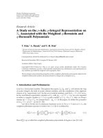
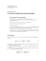
Figure 1: Mean MI(0) of shuffled sequences.
In all three cases, the MI(0) score for a shuffled se-
quence of infinite length would be 0; therefore, the calculated
scores represent the error introduced by sample-size effects.
Figure 1, mean MI(0) of shuffled sequences, shows the aver-
age shuffled sequence scores (i.e., sampling error) in bits for
each method. This figure shows that, as expected, the sam-
pling error tends to decrease as the sequence length increases.
4.1. Significance of MI(0) for protein sequences
To compare the amount of error, in each method we nor-
malized the mean MI(0) scores from Figure 1 by dividing the
mean MI(0) score by the MI(0) score of the sequence used to
generate the shuffles. This ratio estimates the amount of the
sequence MI(0) score attributed to sample-size effects.
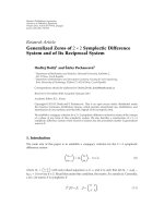
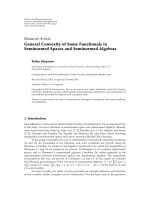
Figure 2, normalized MI(0) of shuffled sequences, com-
pares the effectiveness of our two corrective methods in min-
imizing the sample-size effects. This figure shows that nor-
malization by joint entropy is not as effective as Figure 1 sug-
gests. Despite a large reduction in bits, in most cases, the por-
tion of the score attributed to sampling effects shows only a
minor improvement. Σ
H
still shows a significant reduction in
sample-size effects for most sequences.
Figures 1 and 2 provide insight into trends for the three

methods, but do not answer our question of whether or not
the MI scores are significant. For a given sequence S,weesti-
mated the P value as
P
=
x
N
, (13)
where N is the number of random shuffles and x is the num-
ber of shuffles whose MI(0) was greater than or equal to
MI(0) for S. For this experiment, we choose a sig nificance
cutoff of .05. For a sequence to be labeled significant, no more
than 50 of the 10 000 shuffled versions may have an MI(0)
score equal or larger than the original sequence. We repeated
100 200 300 400 500 600 700 800 900 1000
Sequence length (residue count)
0
0.1
0.2
0.3
0.4
0.5
0.6
0.7
0.8
0.9
1
Mean of MI(0) for shuffles/MI(0) for sequence
Σ
A

literal
Σ
A
litera l, normalized
Σ
H
literal
Figure 2: Normalized MI(0) of shuffled sequences.
this experiment for MI(1), MI(5), MI(10), and MI(15) and
summarized the results in Ta ble 4.
These results suggest that despite the low MI content of
protein sequences, we are able to detect significant MI in a
majority of our sampled sequences at MI(0). The number of
significant sequences decreases for MI(d) as d increases. The
results for the classic MI method are significantly affected by
sampling error. Normalization by joint entropy reduces this
error slightly for most sequences, and using Σ
H
is a much
more effective correction.
5. MEASURING MIV PERFORMANCE THROUGH
PROTEIN CLASSIFICATION
We used sequence classification to evaluate the ability of MI
to characterize protein sequences and to test our hypothe-
sis that MIV characterizes a protein sequence better MI. As
such,ourobjectiveistomeasurethedifference in accuracy
between the methods, rather than to reach a specific classifi-
cation accuracy.
We used the Pfam-A dataset to carry out this compar-
ison. The families contained in the Pfam database vary in

sequence count and sequence length. We removed all fami-
lies containing any sequence of less than 100 residues due to
complications with calculating MI for smal l strings. We also
limited our study to families with more than 10 sequences
and less than or equal to 200 sequences. After filtering Pfam-
A based on our requirements, we were left with 2392 families
to consider in the experiment.
Sequence similarity is the most widely used method of
family classification. BLAST [10] is a popular tool incor-
porating this method. Our method differs significantly, in
that classification is based on a vector of numerical features,
rather than the protein’s residue sequence.
6 EURASIP Journal on Bioinformatics and Systems Biology
Table 4: Sequence significance calculated for significance cutoff .05.
Scoring method
Number of significant sequences (of 1000)
MI(0) MI(1) MI(5) MI(10) MI(15)
Literal-Σ
A
762 630 277 103 54
Normalized
literal-Σ
A
777 657 309 106 60
Literal-Σ
H
894 783 368 162 117
Classification of feature vectors is a well-studied prob-
lem with many available strategies. A good introduction to
many methods is available in [11], and the method chosen

can significantly affect performance. Since the focus of this
experiment is to compare methods of calculating MIV, we
only used the well-established and versatile nearest neighbor
classifier in conjunction with Euclidean distance [12].
5.1. Classification implementation
For classification, we used the WEKA package [11]. WEKA
uses the instance based 1 (IB1) algorithm [13] to imple-
ment nearest neighbor classification. This is an instance-
based learning algorithm derived from the nearest neighbor
pattern classifier and is more efficient than the naive imple-
mentation.
The results of this method can differ from the classic
nearest neighbor classifier in that the range of each attribute
is normalized. This normalization ensures that each attribute
contributes equally to the calculation of the Euclidean dis-
tance. As shown in Tabl e 3, MI scores calculated from Σ
A
have a larger magnitude than those calculated from Σ
H
. This
normalization allows the two alphabets to be used together.
5.2. Sequence classification with MIV
In this experiment, we explore the effectiveness of classifica-
tions made using the correlation measurements outlined in
Section 3.
Each experiment was performed on a random sample of
50 families from our subset of the Pfam database. We then
used leave-one-out cross-validation [14]totesteachofour
classification methods on the chosen families.
In leave-one-out validation, the sequences from a ll 50

families are placed in a t raining pool. In turn, each sequence
is extracted from this pool and the remaining sequences are
used to build a classification model. The extracted sequence
is then classified using this model. If the sequence is placed
in the correct family, the classification is counted as a suc-
cess. Accuracy for each method is measured as
no. of correct classifications
no. of classification attempts
. (14)
We repeated this process 100 times, using a new sampling
of 50 families from Pfam each time. Results are reported for
each method as the mean accuracy of these repetitions. For
each of the 24 combinations of scoring options outlined in
Section 3, we evaluated classification based on MI(0), as well
as MIV
20
. The results for these experiments are summarized
in Tabl e 5, classification Results for MI(0) and MIV
20
.
All MIV
20
methods were more accurate than their MI(0)
counterpar ts. The best method was Σ
H
with hybrid gap scor-
ing with a mean accuracy of 85.14%. The eight best perform-
ing methods used Σ
H
, with the best method based on Σ

A
hav-
ing a mean accuracy of only 66.69%. Another important ob-
servation is that strict gap interpretation performs poorly in
sequence classification. The best strict method had a mean
accuracy of 29.96%—much lower than the other gap meth-
ods.
Our final classification attempts were made using con-
catenations of previously generated MIV
20
scores. We eval-
uated all combinations of methods. The five combinations
most accurate at classification are shown in Ta ble 6. The best
method combinations are over 90% accurate, with the best
being 90.99%. The classification power of Σ
H
with hybrid
gap interpretation is demonstrated, as this method appears
in all five results. Surprisingly, two strict scoring methods ap-
pear in the top 5, despite their poor performance when used
alone.
Based on our results, we made the following observa-
tions.
(1) The c orrelation of non-adjacent pairs as measured
by MIV is significant. Classification based on every
method improved significantly for MIV compared to
MI(0). The highest accuracy achieved for MI(0) was
26.73% and for MIV it was 85.14% (see Table 5).
(2) Normalized MI had an insignificant effect on scores gen-
erated from Σ

H
. Both methods reduce the sample-size
error in estimating entropy and MI for sequences. A
possible explanation for the lack of further improve-
ment through normalization is that Σ
H
is a more ef-
fective corrective measure than normalization. We ex-
plore this possibility further in Section 6.2,werewe
consider entropy for both alphabets.
(3) For the most accurate methods, using the Pfam prior de-
creased accuracy. Despite our concerns about using the
frequency of a short sequence to estimate the marginal
residue probabilities, the results show that these es-
timations better characterize the sequences than the
Pfam prior probability distribution. However, four of
the five best combinations contain a method utilizing
the Pfam prior, showing that the two methods for esti-
mating marginal probabilities are complimentary.
(4) As with sequence-based classification, introducing gaps
improves accuracy. For all methods, removing gap char-
acters with the strict method drastically reduced accu-
racy. Despite this, two of the five best combinations in-
cluded a strict scoring method.
(5) The best scoring concatenated MIVs included both al-
phabets. The inclusion of Σ
A
is significant—all eight
nonstric t Σ
H

methods scored better than any Σ
A
method (see Ta ble 5). The inclusion shows that Σ
A
provides information not included in the Σ
H
and
strengthens our assertion that the different alphabets
characterize different forces affecting protein struc-
ture.
C. Hemmerich and S. Kim 7
Table 5: Classification results for MI(0) and MIV
20
methods. SD represents the standard deviation of the experiment accuracies.
MIV
20
Method
MI(0) accuracy MIV
20
accuracy
rank Mean SD Mean SD
1 Hybrid-Σ
H
26.73% 2.59 85.14% 2.06
2 Normalized hybrid-Σ
H
26.20% 4.16 85.01% 2.19
3 Literal-Σ
H
22.92% 3.41 79.51% 2.79

4 Normalized literal-Σ
H
23.45% 3.88 78.86% 2.79
5 Normalized Hybrid-Σ
H
w/Pfam prior 26.31% 3.95 77.21% 2.94
6 Literal-Σ
H
w/Pfam prior 22.73% 4.90 76.89% 2.91
7 Normalized Literal-Σ
H
w/Pfam prior 22.45% 4.89 76.29% 2.96
8 Hybrid-Σ
H
w/Pfam prior 22.81% 2.97 71.57% 3.15
9 Normalized literal-Σ
A
17.76% 3.21 66.69% 4.14
10 Hybrid-Σ
A
17.16% 3.06 64.09% 4.36
11 Normalized literal-Σ
A
w/Pfam prior 19.60% 3.67 63.39% 4.05
12 Literal-Σ
A
16.36% 2.84 61.97% 4.32
13 Literal-Σ
A
w/Pfam prior 19.95% 2.84 61.82% 4.12

14 Hybrid-Σ
A
w/Pfam prior 23.09% 3.36 58.07% 4.28
15 Normalized hybrid-Σ
A
18.10% 3.08 41.76% 4.59
16 Normalized hybrid-Σ
A
w/Pfam prior 23.32% 3.65 40.46% 4.04
17 Strict-Σ
H
w/Pfam prior 12.97% 2.85 29.96% 3.89
18 Normalized strict-Σ
H
w/Pfam prior 13.01% 2.72 29.81% 3.87
19 Normalized strict-Σ
A
w/Pfam prior 19.77% 3.52 29.73% 3.93
20 Normalized strict-Σ
A
18.27% 2.92 29.20% 3.65
21 Strict-Σ
H
11.22% 2.33 29.09% 3.60
22 Normalized strict-Σ
H
11.15% 2.52 28.85% 3.58
23 Strict-Σ
A
w/Pfam prior 19.25% 3.38 28.44% 3.91

24 Strict-Σ
A
16.27% 2.75 25.80% 3.60
Table 6: Top scoring combinations of MIV methods. All combinations of two MIV methods were tested, with these five methods performing
the most accurately. SD represents the standard dev i ation of the experiment accuracies.
Rank First method Second method Mean accuracy SD
1 Hybrid-Σ
H
Normalized hybrid-Σ
A
w/Pfam prior 90.99% 1.44
2 Hybrid-Σ
H
Normalized strict-Σ
A
w/Pfam prior 90.66% 1.47
3 Hybrid-Σ
H
Literal-Σ
A
w/Pfam prior 90.30% 1.48
4 Hybrid-Σ
H
Literal-Σ
A
90.24% 1.73
5 Hybrid-Σ
H
Strict-Σ
A

w/Pfam prior 90.08% 1.57
6. FURTHER MIV ANALYSIS
In this section, we examine the results of our different meth-
ods of calculating MIVs for Pfam sequences. We first use cor-
relation within the MIV as a metric to compare several of our
scoring methods. We then take a closer look at the effect of
reducing our alphabet size when translating from Σ
A
to Σ
H
.
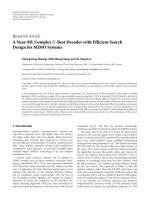
6.1. Correlation within MIVs
We calculated MIVs for 120 276 Pfam sequences using each
of our methods and measured the correlation within each
method using Pearson’s correlation. The results of this anal-
ysis are presented in Figure 3. Each method is represented by
a20
× 20 grid containing each pairing of entries within that
MIV.
The results strengthen our obser vations from the classifi-
cation experiment. Methods that performed well in classifi-
cation exhibit less redundancy between MIV indexes. In par-
ticular, the advantage of methods using Σ
H
is clear. In each
case, correlation decreases as the distance between indexes
increases. For short distances, Σ
A
methods exhibit this to a
lesser degree; however, after index 10, the scores are highly

correlated.
6.2. Effect of alphabets
Not all intraprotein interactions are residue specific. Cline
[2] explored information attributed to hydropathy, charge,
disulfide bonding, and burial. Hydropathy, an alphabet com-
posed of two symbols, was found to contain half as much in-
formation as the 20-element amino acid alphabet. However,
8 EURASIP Journal on Bioinformatics and Systems Biology
5101520
Literal-Σ
A
5
10
15
20
5101520
Normalized litera l-Σ
A
5
10
15
20
5101520
Hybrid-Σ
A
5
10
15
20
5101520

Normalized hybrid-Σ
A
5
10
15
20
0.2
0.4
0.6
0.8
(a)
5101520
Literal-Σ
H
5
10
15
20
5101520
Normalized litera l-Σ
H
5
10
15
20
5101520
Hybrid-Σ
H
5
10

15
20
5101520
Normalized hybrid-Σ
H
5
10
15
20
0.2
0.4
0.6
0.8
(b)
Figure 3: Pearson’s correlation analysis of scoring methods. Note the reduced correlation in the methods based on Σ
H
, which all performed
very well in classification tests.
with only two symbols, the alphabet should be more resistant
to the underestimation of ent ropy and overestimation of MI
caused by finite sequence effects [15].
For this method, a protein sequence is translated using
the process given in Section 3.2. It is important to remem-
ber that the scores generated for entropy and MI are actually
estimates based on finite samples. Because of the reduced al-
phabet size of Σ
H
, we expected to see increased accuracy in
entropy and MI estimations.To confirm this, we examined
the effects of converting random sequences of 100 residues

(a length representative of those found in the Pfam database)
into Σ
H
.
We generated each sequence from a Bernoulli scheme.
Each position in the sequences is selected independently of
any residues selected before it, and all selections are made
randomly from a uniform distribution. Therefore, for every
position in the sequence, al l residues are equally likely to oc-
cur.
By sampling residues from a uniform distribution, the
Bernoulli scheme maximizes entropy for the alphabet size
(N):
H
=−log
2
1
N
. (15)
Since all positions are independent of others, MI is 0.
Knowing the theoretical values of both ent ropy and MI, we
can compare the calculated estimates for a finite sequence to
the theoretical values to determine the magnitude of finite
sequence effects.
We estimated entropy and MI for each of these sequences
and then translated the sequences to Σ
H
. The translated
sequences are no longer Bernoulli sequences because the
residue partitioning is not equal—eight residues fall into one

category and twelve into the other. Therefore, we estimated
the entropy for the new alphabet using this probability distri-
Table 7: Comparison of measured entropy to expected entropy val-
ues for 1000 amino acid sequences. Each sequence is 100 residues
long and was generated by a Bernoulli scheme.
Alphabet
Alphabet
size
Theoretical
entropy
Mean measured
entropy
Σ
A
20 4.322 4.178
Σ
H
2 0.971 0.964
bution. The positions remain independent, so the expected
MI remains 0.
Tab le 7 shows the measured and expected entropies for
both alphabets. The entropy for Σ
A
is underestimated by
.144, and the entropy for Σ
H
is underestimated by only
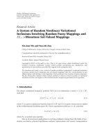
.007. The effect of Σ
H
on MI estimation is much more pro-

nounced. Figure 4 shows the dramatic overestimation of MI
in Σ
A
and high standard deviation around the mean. The
overestimation of MI for Σ
H
is negligible in comparison.
7. CONCLUSIONS
We have shown that residue correlation information can be
used to characterize protein sequences. To model sequences,
we defined and used the mutual information vector (MIV)
where each entry represents the mutual information content
between two amino acids for the corresponding distance. We
have shown that MIV of proteins is significantly different
from random sequences of the same character composition
when the distance between residues is considered. Furthermore,
we have shown that the MIV values of proteins are significant
enough to determine the family membership of a protein se-
quence with an accuracy of over 90%. What we have shown is
simply that the MIV score of a protein is significant enough
C. Hemmerich and S. Kim 9
024681012141618
Residue distance d
0
0.5
1
1.5
2
2.5
MI (d)

Mean MIV for Σ
H
Mean MIV for Σ
A
Figure 4: Comparison of MI overestimation in protein sequences
generated from Bernoulli schemes for gap distances from 0 to
19 residues. The full residue alphabet greatly over-estimates this
amount. Reducing the alphabet to two symbols approximates the
theoretical value of 0.
for family classification—MIV is not a practical alternative to
similarity-based family classification methods.
There are a number of interesting questions to be an-
swered. In particular, it is not clear how to interpret a vector
of mutual information values. It would also be interesting
to study the effect of distance in computing mutual infor-
mation in relation to protein structures, especially in terms
of secondary structures. In our experiment (see Table 4 ), we
have observed that normalized MIV scores exhibit more in-
formation content than nonnormalized MIV scores. How-
ever, in the classification task, normalized MIV scores did
not always achieve better classification accuracy than non-
normalized MIV scores. We hope to investigate this issue in
the future.
ACKNOWLEDGMENTS
This work is part ially supported by NSF DBI-0237901 and
Indiana Genomics Initiatives (INGEN). The authors also
thank the Center for Genomics and Bioinformatics for the
use of computational resources.
REFERENCES
[1] O. Weiss, M. A. Jim

´
enez-Monta
˜
no, and H. Herzel, “Informa-
tion content of protein sequences,” Journal of Theoretical Biol-
ogy, vol. 206, no. 3, pp. 379–386, 2000.
[2] M.S.Cline,K.Karplus,R.H.Lathrop,T.F.Smith,R.G.Rogers
Jr., and D. Haussler, “Information-theoretic dissection of pair-
wise contact potentials,” Proteins: Str ucture, Function and Ge-
netics, vol. 49, no. 1, pp. 7–14, 2002.
[3] L. C. Martin, G. B. Gloor, S. D. Dunn, and L. M. Wahl, “Us-
ing information theory to search for co-evolving residues in
proteins,” Bioinformatics, vol. 21, no. 22, pp. 4116–4124, 2005.
[4] A. Bateman, L. Coin, R. Durbin, et al., “The Pfam protein fam-
ilies database,” Nucleic Acids Research, vol. 32, Database issue,
pp. D138–D141, 2004.
[5] W. R. Atchley, W. Terhalle, and A. Dress, “Positional depen-
dence, cliques, and predictive motifs in the bHLH protein do-
main,” Journal of Molecular Evolution, vol. 48, no. 5, pp. 501–
516, 1999.
[6]O.WeissandH.Herzel,“Correlationsinproteinsequences
and property codes,” Journal of Theore tical Biology, vol. 190,
no. 4, pp. 341–353, 1998.
[7] T.M.CoverandJ.A.Thomas,Elements of Information Theory,
Wiley-Interscience, New York, NY, USA, 1991.
[8] I. Grosse, H. Herzel, S. V. Buldyrev, and H. E. Stanley, “Species
independence of mutual information in coding and noncod-
ing DNA,” Physical Review E, vol. 61, no. 5, pp. 5624–5629,
2000.
[9] M.A.Jim

´
enez-Monta
˜
no, “On the syntactic structure of pro-
tein sequences and the concept of grammar complexity,” Bul-
letin of Mathematical Biology, vol. 46, no. 4, pp. 641–659, 1984.
[10] S. F. Altschul, W. Gish, W. Miller, E. W. Myers, and D. J. Lip-
man, “Basic local alignment search tool,” Journal of Molecular
Biology, vol. 215, no. 3, pp. 403–410, 1990.
[11] I. H. Witten and E. Frank, Data Mining: Practical Machine
Learning Tools and Techniques, Morgan Kaufmann Ser ies in
Data Management Systems, Morgan Kaufmann, San Fran-
cisco, Calif, USA, 2nd edition, 2005.
[12] T. M. Cover and P. Hart, “Nearest neighbor pattern classifica-
tion,” IEEE Transactions on Information Theory, vol. 13, no. 1,
pp. 21–27, 1967.
[13] D. W. Aha, D. Kibler, and M. K. Albert, “Instance-based learn-
ing algori thms,” Machine Learning, vol. 6, no. 1, pp. 37–66,
1991.
[14] R. Kohavi, “A study of cross-validation and bootstrap for ac-
curacy estimation and model selection,” in Proceedings of the
14th International Joint Conference on Artificial Intelligence (IJ-
CAI ’95), vol. 2, pp. 1137–1145, Montr
´
eal, Qu
´
ebec, Canada,
August 1995.
[15] H. Herzel, A. O. Schmitt, and W. Ebeling, “Finite sample ef-
fects in sequence analysis,” Chaos, Solitons & Fractals, vol. 4,

no. 1, pp. 97–113, 1994.