Báo cáo hóa học: " Research Article Detection and Separation of Speech Events in Meeting Recordings Using a Microphone Array" docx

Hindawi Publishing Corporation
EURASIP Journal on Audio, Speech, and Music Processing
Volume 2007, Article ID 27616, 8 pages
doi:10.1155/2007/27616
Research Article
Detection and Separation of Speech Events in Meeting
Recordings Using a Microphone Array
Futoshi Asano,
1
Kiyoshi Yamamoto,
1
Jun Ogata,
1
Miichi Yamada,
2
and Masami Nakamura
2
1
Information Technology Research Institute, National Institute of Advanced Industrial Science and Technology,
Tsukuba Central 2, 1-1-1 Umezono, Tsukuba 305-8568, Japan
2
Advanced Media, Inc., 48F Sunshine 60 Building, 3-1-1 Higashi-Ikebukuro, Toshima-Ku, Tokyo 170-6048, Japan
Received 2 November 2006; Revised 14 February 2007; Accepted 19 April 2007
Recommended by Stephen Voran
When applying automatic speech recognition (ASR) to meeting recordings including spontaneous speech, the performance of ASR
is greatly reduced by the overlap of speech events. In this paper, a method of separating the overlapping speech events by using an
adaptive beamforming (ABF) framework is proposed. The main feature of this method is that all the information necessary for the
adaptation of ABF, including microphone calibration, is obtained from meeting recordings based on the results of speech-event
detection. The performance of the separation is evaluated via ASR using real meeting recordings.
Copyright © 2007 Futoshi Asano et al. This is an open access article distributed under the Creative Commons Attribution License,
which permits unrestricted use, distribution, and reproduction in any medium, provided the original work is properly cited.

1. INTRODUCTION
The analysis, structuring, and automatic transcription of
meeting recordings have attracted considerable attention in
recent years (e.g., [1–5]). Especially for small informal meet-
ings, a major difficulty is that the discussion consists of spon-
taneous speech, and various types of unexpected speech or
nonspeech events may occur. One such event is the responses
by listeners such as “Uh-huh” or “I see” being inserted in
short pauses in the main speech. These responses are some-
times very close to or even overlap the speech of the main
speaker, and it is difficult to remove them by segmentation
in the time domain. Due to the insertion of these small
speech events, the performance of automatic speech recog-
nition (ASR) is sometimes greatly reduced.
In the field of signal processing, various types of sound
separation, such as blind source separation (BSS, e.g., [6])
and adaptive beamforming (ABF, e.g., [7]), have been inves-
tigated. By using these methods, signals from different sound
sources located at different positions can be separated in the
spatial domain, and can thus be effective for the separation
of speech events that overlap in the time domain.
In most of these previous approaches, a general frame-
work of sound separation for a general scenario, in which
the target signal and interference coexist in an unknown en-
vironment, was treated. Especially, BSS utilizes (almost) no
prior knowledge on the observed signal and the sources, and
can thus be applied to a wide variety of applications. Due to
this difficult blind scenario, however, the BSS approach has
atradeoff that requires longer adaptation (learning) time. In
the meeting situation addressed in this paper, the length of

the overlapping section of speech events is often very short
and the data sufficient for BSS may not be obtained.
In the ABF approach, the condition assumed in the BSS
scenario is somewhat relaxed, and the spatial information
of the target is provided by the user while the spatial in-
formation of the interference is estimated in the adaptation
process. To provide the spatial information on the target, a
calibration based on measurement is usually employed. In
measurement-based calibration, precise measurement must
be done for every individual microphone array, and this
hinders mass production. For the generalized sidelobe can-
celler (GSC), online self-calibration algorithms have been
proposed [8–10]. Such algorithms are necessary for a general
scenario in which only the mixture of target signal and inter-
ference can be observed. However, if the target signal alone
can be observed, it is obvious that the calibration process can
be much simpler and easier.
Also, in the estimation of the spatial information of the
interference, the adaptation wil l be easier and more efficient
when the interference alone can be observed. In a general sce-
nario in which this “target-free” interference is not available,
2 EURASIP Journal on Audio, Speech, and Music Processing
Detection of
speech event
Sound source
clustering
Sound
localization
Estimation of
steering vector

Estimation of
noise correlation
Filtering
Information on
speech events
Range of
speaker
Input signal
Detection Separation
Separated signal
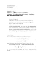
Figure 1: Outline of the proposed method.
the class of ABF which can be used in the mixed situation
such as a minimum variance (MV) beamformer or a GSC
must be used. When the interference alone can be observed,
on the other hand, the classical maximum-likelihood (ML)
beamformer, which outperforms the other types of beam-
formers in this limited situation [11], can be used. In [12],
an audio-visual information fusion was employed to detect
the absence of the target so that the interference alone could
be observed.
In this paper, a new approach for the separation of over-
lapping speech events in meetings based on the ML-type ABF
framework is proposed [13]. As described above, if “pure” in-
formation on the target and interference sources is available,
the calibration and the adaptation process is much easier and
more effective. In a usual small-sized meeting treated in this
paper, there are some advantages that can be utilized in the
automatic calibration and adaptation of ABF as follows:
(i) In the neighborhood of overlapping speech events,
sections in which the target speaker and the com-

peting speaker are speaking on their own are usual ly
found (these sect ions are termed “single-talking” sec-
tions hereafter).
(ii) The movements of speakers are relatively small.
(iii) The processing does not have to be real-time.
Utilizing these characteristics peculiar to meeting recordings,
in this paper, the ABF framework is modified so that it is suit-
able for the separation of speech events in a meeting record-
ing. The basic idea is that the pure information on the tar-
get and the interference is extracted from the single-talking
sections before or after the overlapping section. Regarding
the automatic calibration, even if only the target source is
active, the calibration cannot be accomplished by using the
cross-spectrum between the microphones due to the pres-
ence of the room reverberation and background noise. In
this paper, a method of automatic calibration based on the
subspace appr oach is proposed. The effect of reducing re-
verberation and background noise by the subspace approach
has been demonstrated in [14]. Also, a selection algorithm of
an appropriate single-talking section effective for the separa-
tion of overlapping speech events is proposed. This selection
algorithm is essential to the proposed method since the lo-
cation information included in the overlapping section and
that included in the single-talking sections may differ due to
the fluctuation of the position of the speakers.
An important issue in the analysis of meetings is the au-
tomation of the analyzing process. By employing the pro-
posed method including self-calibr a tion of the microphone
array, the signal processing component of the system is al-
most completely automated. The application of a beam-

former to the reduction of overlapping speech in meeting
recordings has already been proposed in the previous stud-
ies (e.g., [1]). However, the viewpoint of the automation of
the process has not been mentioned in previous approaches.
2. OVERVIEW OF THE PROPOSED METHOD
In this paper, meetings are recorded by using a microphone
array and are stored in a computer. Figure 1 shows an out-
line of the proposed method. In the first half of the method
(left half of Figure 1), speech events are detected based on
sound localization, and the speaker in each event is identi-
fied (Section 3). In the second half (right half of Figure 1), the
overlapping sections of the speech events are separated based
on the information regarding the detected speech events
(Section 4). ASR is then applied to separated speech events
for evaluation (Section 5).
3. DETECTION OF SPEECH EVENTS
3.1. Sound localization
Meeting data recorded by using a microphone array are seg-
mented into time blocks. The spatial spectrum for each block
is then estimated by the MUSIC method [15]. The MUSIC
spectrum is obtained by
P(θ, ω,
t) =
v
H
(θ, ω)v(θ, ω)


v
H

(θ, ω)E
n


2
. (1)
The symbols ω and
t denote the indices for the frequency and
the time block, respectively. The matrix E
n
consists of the
eigenvectors of the noise subspace of the spatial correlation
matrix (eigenvectors corresponding to the smallest M
− N
eigenvalues where M and N denote the number of micro-
phones and the number of active sound sources, resp.). The
spatial correlation matrix is defined as
R
= E

x(ω, t)x
H
(ω, t)

. (2)
The vector x(ω, t)
= [X
1
(ω, t), , X
M

(ω, t)]
T
is termed the
input vector, where X
m
(ω, t) denotes the short-term Fourier
transform of the mth microphone input. The index t corre-
sponds to each Fourier transform within a single time block.
The vector v(θ, ω) is termed the steering vector, which
consists of the transfer function of the direct path from the
(virtual) sound source located at angle θ to the microphones
as follows:
v(θ, ω)
=

V
1
(θ, ω)e
jωτ
1
(θ)
, , V
M
(θ, ω)e
jωτ
M
(θ)

T
,(3)

Futoshi Asano et al. 3
where V
m
(θ, ω)andτ
m
(θ) denote the gain and the time de-
lay at the mth microphone. For sound localization, the set
of steering vectors in the range of angles of interest (e.g.,
every 1 degree from 0
◦
to 359
◦
, 360 directions) is required.
The steering vector can be calculated based on the geometric
configuration of a microphone array and a (virtual) sound
source. This calculated steering vector is hereafter termed the
prototype steering vector (PSV) for the sake of convenience.
PSV differs from the actual one due to the gain difference
of the microphones, complicated acoustics such as diffrac-
tion from the array surface, and geometric errors. An alter-
native way of obtaining a set of steering vectors is calibration
using a test signal such as a TSP (time-stretched pulse) sig-
nal [16]. While the steering vectors measured in the calibra-
tion are more precise than the PSVs, the calibration is time-
consuming and is not practical for mass production. Since
sound localization is less sensitive to the above-described er-
rors than sound separation, PSVs are employed for the sound
localization. In (3), the gain difference is assumed to be zero,
that is, V
1

(θ, ω) =···=V
M
(θ, ω) = 1, and the time differ-
ence τ
m
(θ) is calculated by the microphone array configura-
tion.
After obtaining the spatial spe ctrum at each frequency,
P(θ, ω,
t) is averaged over the frequencies of interest so that
the spatial spectrum for the broadband signal is obtained:
P(θ, t) =
1
N
ω
ω
H

ω=ω
L
λ
ω
P(θ, ω, t). (4)
The symbols [ω
L
, ω
H
]andN
ω
denote the frequency range of

interest and the number of frequency bins, respectively. The
symbol λ
ω
is the frequency weight. In this paper, the square
root of the sum of the eigenvalues for the signal subspace is
used as λ
ω
[12]. By detecting the peaks in the spatial spec-
trum
P(θ, t), the location of the active sound sources (speak-
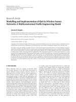
ers) in each time block can be estimated. An example of the
estimated location of the speakers in a meeting recording is
shown in Figure 2(a).
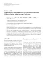
3.2. Clustering of sound sources
By clustering the estimated location of the sound sources col-
lected from the entire meeting, the range of each speaker
is determined. For clustering, k-means is used in this pa-
per. The number of participants is given to the system as the
number of clusters. An example of the distribution of the es-
timated locations and the clustering is depicted in Figure 3.
3.3. Detection of speech events
From the estimated sound source locations (Figure 2(a))and
the range of speakers (Figure 3), the active speakers are iden-
tified in each block. Adjacent blocks with the same active
speakers are then merged into a single speech event. The
adjacent speech events with small gaps (short pauses) are
also merged. An example of the detected and merged speech
events is shown in Figure 2(b).
130 140 150 160 170 180
Time (s)

180
120
60
0
−60
−120
−180
Direction (degree)
(a) Peaks in spatial spectrum in every block
130 140 150 160 170 180
Time (s)
6
5
4
3
2
1
Speaker number
(b) Detected speech events
Figure 2: An example of detected speech events.
4. SEPARATION OF SPEECH EVENTS
In this section, overlapping speech events are separated using
an adaptive/nonadaptive beamformer based on the informa-
tion of the detected speech events.
Some types of beamformers are described in the fre-
quency domain as follows (e.g., [7]):
y(ω, t)
= w
H
x(ω, t), (5)

w
=
R
−1
n
a
a
H
R
−1
n
a
. (6)
Here, x(ω, t)andy(ω, t) represent the input and output of
the beamformer, respectively. Vector w consists of the beam-
former coefficients. Steering vector a consists of the trans-
fer function of the direct path from the target speaker to the
microphones in the same way as (3). Matrix R
n
is termed the
noise spatial correlation matrix,
R
n
= E

x
n
(ω, t)x
H
n

(ω, t)

,(7)
where x
n
(ω, t) is the input vector corresponding to the noise
sources (competing speakers).
4 EURASIP Journal on Audio, Speech, and Music Processing
−100 0 100
Direction (degree)
0
500
1000
1500
2000
2500
3000
3500
Number of blocks
Figure 3: Distribution of the estimated active sound sources and
the results of clustering.
In the next sections, a method of obtaining the infor-
mation required for constructing the beamformer coefficient
vector w,namely,a and R
n
,isproposed.
4.1. Estimation of steering vector a (calibration)
As described above, the steering vector for the target speaker,
a, is required for updating (6). In this and the subsequent
sections, the indices ω and t are omitted for the sake of sim-

plicity. As described in Section 3.1, a PSV for the target,
v,
that is selected in the sound localization process, is a rough
approximation of the actual steering vector, and thus can-
not be u sed for speech e vent separa tion (see the results of the
experiment described in Section 5). In this subsection, there-
fore, the steering vector for the target is estimated from the
data of meeting recordings.
For the sake of convenience, the time block in which
the overlapping speech events are to be separated is termed
the “current block.” In the neighborhood of the current
block, the time blocks in which the target alone is speaking
(single-talking blocks) are expected to be found, as shown
in Figure 4(a). The steering vector for the target can be es-
timated using the data in these blocks. Single-talking blocks
can b e easily found by using the speech-event information
obtained in Section 3.
Once a single-talking block is found, an estimate of the
target steering vector can be obtained as the eigenvector of
the spatial correlation matrix corresponding to the largest
eigenvalue. This can be easily understood from the subspace
structure of the spatial correlation matrix as follows (e.g.,
[7]). Figure 5 shows the relation of the steering vectors and
the eigenvectors of the spatial correlation matrix. This exam-
ple shows the case of N
= 2(numberofsoundsources)and
Targe t
Interference
Speaker
e

1
Current
block
v
Candidates
Time
(a)
Targe t
Interference
Speaker
Current
block
Candidates
Time
CK(1)
(b)
Figure 4: Estimation of (a) the steering vector and (b) the noise
correlation.
M = 3 (number of microphones). It is assumed that the in-
put signal x is modeled as
x
= As + n,(8)
where matrix A consists of the steering vectors as A
=
[a
1
, a
2
]andvectors consists of the source spectrum as
s

= [S
1
(ω, t), S
2
(ω, t)]
T
.Vectorn represents the background
noise. It is known that the eigenvectors corresponding to the
largest N eigenvalues become the basis of the signal subspace
spanned by the steering vectors
{a
1
, , a
N
}. In this example,
eigenvectors e
1
and e
2
become the basis of the signal subspace
spanned by steering vectors a
1
and a
2
. From this, it is obvi-
ous that when a speaker is speaking on his/her own (N
= 1),
the dimension of the signal subspace becomes one and the
direction of eigenvector e
1

matches that of steering vector a
1
.
Therefore, the steering vector can be estimated by finding a
single-talking block for the target and extracting the eigen-
vector corresponding to the largest eigenvalue.
Since there will be multiple single-talking blocks in the
neighborhood of the current block, as shown in Figure 4(a),
the most appropriate steering vector must be chosen from
the set of the estimated steering vectors. This set of the es-
timatesisdenotedasΨ
= [e
1
(1), , e
1
(L)], and is termed
candidates. The symbol L denotes the number of candidates.
In this paper, the optimal steering vector is chosen so that it
is closest to the PSV for the target,
v, that is chosen in the
localization process as follows:
a = arg max
e
1
∈Ψ
v
H
e
1
v

H
v
. (9)
Futoshi Asano et al. 5
e
3
e
2
e
1
e
1
e
2
As
x
n
Signal subspace
Figure 5: Relation of steering vectors and eigenvectors.
Since small movements of the speaker are expected during
the meeting, the steering vector whose corresponding loca-
tion is the closest to that of the target in the current block is
expected to be selected by using (9).
The procedure for estimating the steering vector can be
summarized as follows.
(1) Find single-talking blocks based on the speech event
information.
(2) Calculate the correlation matrix R
= E[xx
H

].
(3) Perform eigenvalue decomposition on R and extract
the eigenvector e
1
corresponding to the largest eigen-
value.
(4) Select the optimum steer ing vector using (9).
4.2. Estimation of the noise spatial correlation R
n
Since x
n
(ω, t) cannot be observed s eparately in the current
block, the ideal noise correlation R
n
is also not available.
In a manner similar to the estimation of the steering vec-
tor, the noise correlation is estimated from the neighbor-
hood of the current block. First, the blocks in which the
overlapping sp eaker (noise source) is speaking and the target
speaker is not speaking are found based on the information
of the speech events as depicted in Figure 4(b). The set of
the spatial correlations calculated in these blocks is denoted
as Φ
= [K(1), , K(L)]. When the noise correlation se-
lected from these candidates has spatial characteristics close
to those of the noise in the current block, the beamformer be-
comes an approximation of the maximum-likelihood (ML)
adaptive beamformer.
In addition to the set of the candidates Φ, two other noise
correlation candidates are taken into account to enhance the

performance of the separation and the speech enhancement.
The first one is the identity matrix I, which is the theoretical
noise correlation when the noise is spatially white. A beam-
former using I is termed a delay-and-sum (DS) beamformer.
Even when the target speaker is speaking on his/her own,
there is room reverberation that reduces the performance
of ASR. By applying this beamformer in the sing le-talking
blocks, the effect of speech enhancement is expected.
Another candidate is the correlation calculated in the
current block. This correlation is denoted as C, and the
beamformer using C is termed a minimum variance (MV)
beamformer. The correlation C differs from the ideal noise
correlation R
n
since not only the noise but also the target
signal is included in C. When the level of the target is com-
parable to or larger than that of the noise, the MV beam-
former causes significant distortion of the target signal. On
the other hand, when the noise is dominant in the current
block, R
n
 C, and the noise is effectively reduced since
the characteristics of noise used in the beamformer perfectly
match those of the current block. The characteristics of these
three types of beamformers are summarized in Ta ble 1.
For selecting the noise correlation from the candidates
described above, a criterion similar to that used in the MV
beamformer, that is, the output power of the beamformer in
the current block, is used as follows:


R
n
= arg min
R
n
∈Φ,I,C
w
H
Cw, (10)
where w
=
R
−1
n
a
a
H
R
−1
n
a
. (11)
In (10), w
H
Cw represents the output power of the beam-
former. As a steering vector in the beamformer coefficient
vector w, the one selected in the prev ious subsection,
a,is
used. Since only the output power is taken into account in
(10), C is selected in most cases and a distortion is imposed

on the target signal. Therefore, C is included as a candidate
only when the target signal is absent (short pauses in speech
events).
The procedure for estimating the noise correlation can be
summarized as follows.
(1) Find time blocks in which the target is absent and the
noise is present.
(2) Calculate the correlation in the above time blocks and
form the candidates Φ
= [K(1), , K(L)] (ML).
(3) Add I to the candidates (DS).
(4) Add C to the candidates only when the target is absent
in the current block (MV).
(5) Select the noise correlation from among the candidates
using (10).
4.3. Filtering
Using the estimated steering vector
a and the noise correla-
tion

R
n
, the beamformer coefficient vector w is updated in
every block using (6). The microphone array inputs are then
filtered by the updated coefficient vector using (5). In ac-
tual filtering, the beamformer coefficient vector w is inverse-
Fourier-transformed into the time domain, and (5)iscon-
ducted in the time domain.
5. EXPERIMENT
5.1. Condition

The meeting recorded and analyzed was a “group interview,”
such as that used for Japanese market research. The language
used was Japanese. In such a meeting, a professional inter-
viewer asks questions regarding a product and has a dis-
cussion with interviewees. The number of interviewees in
the recorded meeting was five. T he interviewer was female
while all the interviewees were male (university students).
6 EURASIP Journal on Audio, Speech, and Music Processing
The meeting was recorded in an ordinary meeting room with
a reverberation time of approximately 0.5 second. The length
of the meeting was 104 minutes. Fifty nine percent of the
time blocks were classified as the overlapping blocks. (The
detected overlapping blocks differ from the actual blocks
with overlapping speech since the presence of any sound
other than target speech was detected as an overlap.)
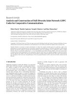
Figure 6 shows the input device used for the recording,
which consists of a microphone array and a camera array
(PointGray Research, Ladybug-2). The microphone array is
circular in shape with a diameter of 15 cm and consists of
eight omnidirectional microphones (Sony, ECM-C115). The
sampling frequency was 16 kHz. The distance between the
microphone array and the participants was 1.0–1.5 m.
In the analysis and separation, the length of the time
block was 0.5 second with an overlap of 0.25 second with
the succeeding block. The length of the Fourier tr a nsform
was 512 points (32 milliseconds). The processing time for the
detection and separation for a single session (104 minutes)
was approximately 5.5 hours (processed by a PC with Xeon
2.8 GHz). In the overlapping sections, only the signals from
the two speakers with the largest and the second largest pow-

ers were separ ated and recognized, regardless of the actual
number of active sound sources for the sake of convenience.
In the ASR used for evaluation, an HMM-based recog-
nizer was used. For the initial acoustic model, a tied-state
triphone (1500 states) was trained on about 60 hours of
speech from our meeting corpus. For the language model
(LM) in the recognizer, b oth an open language model and
a closed language model trained with the transcription of
this meeting by a human listener were used. Although the
use of the closed LM was not practical in terms of the ap-
plication, it was employed to focus on the acoustic aspect of
the speech-event separation. For the open LM, a 14 K-word
trigram was trained on a general spontaneous speech cor-
pus (3.41 MB in text size) plus those of eight group interview
sessions (432 Kb). For the closed LM, on the other hand, a
1.4 K-word trigram was trained from data in a single group
interview session used in the evaluation (55 kB). The topic
of the group interview in the evaluation was about cellular
phones while those of the group interviews in the open LM
were various but covered the cellular phone (the data used
for the closed LM and that for the open LM did not overlap).
The speech events with a duration of more than 5 seconds
(367 speech events) were subjected to ASR for the evaluation.
5.2. Results
Table 2 shows the results of evaluation using ASR. In the
columns labeled “without AM adaptation,” the output of one
of the microphones and the separated output are compared.
In the case of “before separation,” the microphone closest
to the speaker was selected from among the eight micro-
phones based on the localization results. In the compari-

son between “before separation” and “after separation,” the
word-accuracy score was improved by appro ximately 19% in
the closed LM and 12% in the open LM.
Figure 6: Input device used for the recording.
In the columns of “with AM adaptation,” unsupervised
adaptation was conducted on the acoustic model (AM) of
ASR. For the adaptation, M LLR (maximum-likelihood lin-
ear regression) + MAP (maximum a posteriori) [17, 18]were
used. For the case of “entire data,” data of all 367 speech
events were used for the adaptation. For the case of “each
participant,” the speech event data were classified into each
participant, and the six AMs were individually trained us-
ing the data for each participant. Compared with the case of
without AM adaptation, the score was further improved by
approximately 4%. By employing the individual adaptation,
a slight improvement (1%) was observed compared with the
adaptation using all the data.
As described in Section 4.2, one of the three types of
beamformers, that is, DS, ML, and MV, was selected in each
frequency bin at each time block independently by select-
ing the noise spatial correlation from
{K(1), , K(L)}(ML),
I(DS), and C(MV). Table 1 shows the ratio of the selected
beamformer algorithms, namely,
Ratio
=
Number of times of ML/DS/MV being selected
Number of total processed blocks × Number of frequency bins
.
(12)

Figure 7 shows a comparison of the beamformer algo-
rithms. The proposed method in which the beamformer is
selected from among the all three types is denoted as “DS +
ML+MV.” On the other hand, “DS+ML” denotes the case in
which the beamformer is limited to DS and ML. Comparing
“DS + ML + MV” with “DS + ML,” only a slight difference
was found, though “DS + ML + MV” sometimes yielded a
better noise reduction performance in the noise-dominant
blocks according to the informal listening tests. Comparing
the adaptive+nonadaptive beamformer (DS + ML + MV or
Futoshi Asano et al. 7
Table 1: Selected beamformer algorithm and its characteristics.
DS ML MV
Ratio (%) 38.90 51.64 9.46
Signal distortion Small Small
∗
Large
Noise reduction
Small Large
∗
Large
Effective against
Omnidirectional noise
such as reverberation
Directional noise such as speech
from a competing speaker
Directional and dominant
noise such as sound of cough
∗
Theoretically, the ML beamformer shows small signal distortion and large noise reduction. However, for the practical case with approximation as usedin

this paper, the performance of the ML beamformer is in between that of the DS and MV beamformers.
Table 2: Evaluation using ASR (word accuracy (%)). AM: acoustic model; LM: language model.
Without AM adaptation With AM adaptation
LM Before separation After separation Entire data Each participant
Closed 51.09 70.35 74.42 75.69
Open
23.41 35.69 39.52 41.41
020406080
Word accuracy (%)
28.22
50.71
70.51
70.35
66.08
51.09
DS+ML(PSV)
DS(PSV)
DS+ML+MV
DS+ML
DS
No. proc.
Figure 7: Word accuracy for different beamformer combinations.
DS + ML) with the nonadaptive beamformer (DS), improve-
ment of approximately 5% was found for the adaptive +
non-adaptive beamformer. In the cases of “DS(PSV)” and
“DS + ML(PSV),” PSVs were used instead of the estimated
steering vectors. In PSV, only geometric information on the
microphone array was used to obtain the steering vectors.
From these, the effect of estimating the steering vector pro-
posed in this paper can be seen.

6. CONCLUSION
In this paper, a method of separating overlapping sp eech
events in a meeting recording was proposed and evaluated
via ASR. This method utilizes the characteristics peculiar
to meeting recordings and the information on the speech
events detected prior to the separation. Three types of adap-
tive/nonadaptive beamforming are fused so that the process-
ing is effective with both overlapping speech events and room
reverberation. As a result of evaluation experiments using
ASR, the combination of “DS + ML” or “DS + ML + MV”
was found to show an improvement of around 12% (open
LM) and 19% (closed LM) in word accuracy compared with
the single-microphone recording.
As a future work, a method of preparing a language
model in ASR appropriate for each topic of a meeting should
be investigated. Use of visual information is another interest-
ing topic to be investigated in the future. In this paper, the
seats of the meeting participants were assumed to be fixed.
In an informal meeting, par ticipants may move to other po-
sitions, or a new person may begin participating halfway
through the meeting. These dynamic changes can p ossibly
be solved by using visual information as well as acoustic in-
formation.
ACKNOWLEDGMENT
This research was partly supported by JSPS Kakenhi(A), no.
18200007.
REFERENCES
[1] D.C.MooreandI.A.McCowan,“Microphonearrayspeech
recognition: experiments on overlapping speech in meetings,”
in Proceedings of IEEE International Conference on Acoustics,

Speech, and Signal Processing (ICASSP ’03), vol. 5, pp. 497–500,
Hong Kong, April 2003.
[2] A. Dielmann and S. Renals, “Dynamic Bayesian networks for
meeting structuring,” in Proceedings of the IEEE International
Conference on Acoustics, Speech, and Signal Processing (ICASSP
’04), vol. 5, pp. 629–632, Montreal, Que, Canada, May 2004.
[3] J. Ajmera, G. Lathoud, and I. McCowan, “Clustering and seg-
menting speakers and their locations in meetings,” in Proceed-
ings of the IEEE International Conference on Acoustics, Speech,
and Signal Processing (ICASSP ’04), vol. 1, pp. 605–608, Mon-
treal, Que, Canada, May 2004.
[4] M. Katoh, K. Yamamoto, J. Ogata, et al., “State estima-
tion of meetings by information fusion using Bayesian net-
work,” in Proceedings of the 9th European Conference on Speech
Communication and Technology, pp. 113–116, Lisbon, Portu-
gal, September 2005.
[5] T. Hain, J. Dines, G. Garau, et al., “Transcription of confer-
ence room meetings: an investigation,” in Proceedings of the
8 EURASIP Journal on Audio, Speech, and Music Processing
9th European Conference on Speech Communication and Tech-
nology (EUROSPEECH ’05), pp. 1661–1664, Lisbon, Portugal,
September 2005.
[6] S. Haykin, Ed., Unsupervised Adaptive Filtering, Vol. 1,John
Wiley & Sons, New York, NY, USA, 2000.
[7] D. H. Johnson and D. E. Dudgeon, Array Signal Processing,
Prentice-Hall, Englewood Cliffs, NJ, USA, 1993.
[8] O. Hoshuyama, A. Sugiyama, and A. Hirano, “A robust adap-
tive beamformer for microphone arrays with a blocking ma-
trix using constrained adaptive filters,” IEEE Transactions on
Signal Processing, vol. 47, no. 10, pp. 2677–2684, 1999.

[9] P. Oak and W. Kellermann, “A calibration method for robust
generalized sidelobe cancelling beamformers,” in Proceedings
of International Workshop on Acoustic Echo and Noise Con-
trol (IWAENC ’05), pp. 97–100, Eindhoven, The Netherlands,
September 2005.
[10] S. Gannot and I. Cohen, “Speech enhancement based on the
general transfer function GSC and postfiltering,” IEEE Trans-
actions on Speech and Audio Processing, vol. 12, no. 6, pp. 561–
571, 2004.
[11] F. Asano, S. Hayamizu, T. Yamada, and S. Nakamura, “Speech
enhancement based on the subspace method,” IEEE Transac-
tions on Speech and Audio Processing, vol. 8, no. 5, pp. 497–507,
2000.
[12] F. Asano, K. Yamamoto, I. Hara, et al., “Detection and separa-
tion of speech event using audio and video information fusion
and its application to robust speech interface,” EURASIP Jour-
nal on Applied Signal Processing, vol. 2004, no. 11, pp. 1727–
1738, 2004.
[13] F. Asano and J. Ogata, “Detection and separation of speech
events in meeting recordings,” in Proceedings of the 9th In-
ternational Conference on Spoken Language Processing (ICSLP
’06), pp. 2586–2589, Pittsburgh, Pa, USA, September 2006.
[14] F. Asano, S. Ikeda, M. Ogawa, H. Asoh, and N. Kitawaki,
“Combined a pproach of array processing and independent
component analysis for blind separation of acoustic signals,”
IEEE Transactions on Speech and Audio Processing, vol. 11,
no. 3, pp. 204–215, 2003.
[15] R. O. Schmidt, “Multiple emitter location and signal param-
eter estimation,” IEEE Transactions on Antennas and Propaga-
tion, vol. 34, no. 3, pp. 276–280, 1986.

[16] Y. Suzuki, F. Asano, H Y. Kim, and T. Sone, “An optimum
computer-generated pulse signal suitable for the measurement
of very long impulse responses,” Journal of the Acoustical Soci-
ety of America, vol. 97, no. 2, pp. 1119–1123, 1995.
[17] C. J. Leggetter and P. C. Woodland, “Maximum likelihood
linear regression for speaker adaptation of continuous den-
sity hidden Markov models,” Computer Speech and Language,
vol. 9, no. 2, pp. 171–185, 1995.
[18] J L. Gauvain and C H. Lee, “Maximum a posteriori esti-
mation for multivariate Gaussian mixture observations of
Markov chains,” IEEE Transactions on Speech and Audio Pro-
cessing, vol. 2, no. 2, pp. 291–298, 1994.