Báo cáo hóa học: " Research Article Multimicrophone Speech Dereverberation: Experimental Validation" docx

Hindawi Publishing Corporation
EURASIP Journal on Audio, Speech, and Music Processing
Volume 2007, Article ID 51831, 19 pages
doi:10.1155/2007/51831
Research Article
Multimicrophone Speech Dereverberation:
Experimental Validation
Koen Eneman
1, 2
and Marc Moonen
3
1
ExpORL, Department of Neurosciences, Katholieke Universiteit Leuven, O & N 2, Herestraat 49 bus 721,
3000 Leuven , Belgium
2
GroupT Leuven Engineering School, Vesaliusstraat 13, 3000 Leuven, Belgium
3
SCD, Department of Electr ical Engineering (ESAT), Faculty of Engineering, Katholieke Universiteit Leuven,
Kasteelpark Arenberg 10, 3001 Leuven, B elgium
Received 6 September 2006; Revised 9 January 2007; Accepted 10 April 2007
Recommended by James Kates
Dereverberation is required in various speech processing applications such as handsfree telephony and voice-controlled systems,
especially when signals are applied that are recorded in a moderately or highly reverberant environment. In this paper, we com-
pare a number of classical and more recently de veloped multimicrophone dereverberation algorithms, and validate the different
algorithmic settings by means of two performance indices and a speech recognition system. It is found that some of the classical
solutions obtain a moderate signal enhancement. More advanced subspace-based dereverberation techniques, on the other hand,
fail to enhance the signals despite their high-computational load.
Copyright © 2007 K. Eneman and M . Moonen. This is an open access article distributed under the Creative Commons Attribution
License, which permits unrestricted use, distribution, and reproduction in any medium, provided the original work is properly
cited.
1. INTRODUCTION

In various speech communication applications such as tele-
conferencing, handsfree telephony, and voice-controlled sys-
tems, the signal quality is degraded in many ways. Apart
from acoustic echoes and background noise, reverberation
is added to the signal of interest as the signal propagates
through the recording room and reflects off walls, objects,
and people. Of the different types of signal deterioration that
occur in speech processing applications such as teleconfer-
encing and handsfree telephony, reverberation is probably
least disturbing at first sight. However, rooms with a mod-
erate to high reflectivity reverberation can have a clearly neg-
ative impact on the intelligibility of the recorded speech,
and can hence significantly complicate conversation. Dere-
verberation techniques are then called for to enhance the
recorded speech. Performance losses are also observed in
voice-controlled systems whenever signals are applied that
are recorded in a moderately or highly rev erberant environ-
ment. Such systems rely on automatic speech recognition
software, which is typically trained under more or less ane-
choic conditions. Recognition rates therefore drop, unless
adequate dereverberation is applied to the input signals.
Many speech dereverberation algorithms have been de-
veloped over the last decades. However, the solutions avail-
able today appear to be, in general, not very satisfactory,
as will be illust rated in this paper. In the literature, dif-
ferent classes of dereverberation algorithms have been de-
scribed. Here, we will focus on multimicrophone derever-
beration algorithms, as these appear to be most promising.
Cepstrum-based techniques were reported first [1–4]. They
rely on the separability of speech and acoustics in the cep-

stral domain. Coherence-based dereverberation algorithms
[5, 6] on the other hand, can be applied to increase listen-
ing comfort and speech intelligibility in reverberating envi-
ronments and in diffuse background noise. Inverse filtering-
based methods attempt to invert the acoustic impulse re-
sponse, and have been reported in [7, 8]. However, as the
impulse responses are known to be typically nonminimum
phase they have an unstable (causal) inverse. Nevertheless, a
noncausal stable inverse may exist. Whether the impulse re-
sponses are minimum phase depends on the reverberation
level. Acoustic beamforming solutions have been proposed
in [9–11]. Beamformers were mainly designed to suppress
background noise, but are known to partially dereverber-
ate the signals as well. A promising matched filtering-based
2 EURASIP Journal on Audio, Speech, and Music Processing
speech dereverberation scheme has been proposed in [12].
The algorithm relies on subspace tracking and shows im-
proved dereverberation capabilities with respect to classical
solutions. However, as some environmental parameters are
assumed to be known in advance, this approach may be less
suitable in practical applications. Finally, over the last years,
many blind subspace-based system identification techniques
have been developed for channel equalization in digital com-
munications [13, 14]. These techniques can be applied to
speech enhancement applications as well [15], be it with lim-
ited success so far.
In this paper, we give an overview of existing derever-
beration techniques and discuss more recently developed
subspace and frequency-domain solutions. The presented al-
gorithms are compared based on two performance indices

and are evaluated with respect to their ability to enhance
the word recognition rate of a speech recognition system.
In Section 2, a problem statement is given and a general
framework is presented in which the different derev erbera-
tion algorithms can be cast. The dereverberation techniques
that have been selected for the evaluation are discussed in
Section 3. The speech recognition system and the perfor-
mance indices that are used for the evaluation are defined
in Section 4 . Section 5 describes the experiments based on
which dereverberation algorithms have been evaluated and
discusses the experimental results. The conclusions are for-
mulated in Section 6.
2. SPEECH DEREVERBERATION
The signal quality in various speech communication appli-
cations such as teleconferencing, handsfree telephony, and
voice-controlled systems is compromised in many ways. A
first type of disturbance are the so-called acoustic echoes,
which arise whenever a loudspeaker signal is picked up by
the microphone(s). A second source of signal deterioration
is noise and disturbances that are added to the signal of in-
terest. Finally, additional signal degradation occurs when re-
verberation is added to the signal as it propagates through the
recording room reflecting off walls, objects, and people. This
propagation results in a signal attenuation and spectral dis-
tortion that can be modeled well by a linear filter. Nonlinear
effects are typically of second-order and mainly stem from
the nonlinear characteristics of the loudspeakers. The linear
filter that relates the emitted signal to the received signal is
called the acoustic impulse response [16] and plays an im-
portant role in many signal enhancement techniques. Often,

the acoustic impulse response is a nonminimum phase sys-
tem, and can therefore not be causally inverted as this would
lead to an unstable realization. Nevertheless, a noncausal sta-
ble inverse may exist. Whether the impulse response is a min-
imum phase system depends on the reverberation level.
Acoustic impulse responses are characterized by a dead
time followed by a large number of reflections. The dead time
is the time needed for the acoustic wave to propagate from
source to listener via the shortest, direct acoustic path. After
the direct path impulse a set of early reflections are encoun-
tered, whose amplitude and delay are strongly determined by
x
h
1
n
1
+
y
1
e
1
+
x
.
.
.
.
.
.
h

M
+
y
M
e
M
n
M
Compensator C
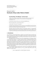
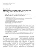
Figure 1: Multichannel speech dereverberation setup: a speech sig-
nal x is filtered by acoustic impulse responses h
1
···h
M
, resulting in
M microphone signals y
1
···y
M
. Typically, also some background
noises n
1
···n
M
are picked up by the microphones. Dereverbera-
tion is aimed a t finding the appropriate compensator C to retrieve
the original speech signal x and to undo the filtering by the impulse
responses h
m
.

the shape of the recording room and the position of source
and listener. Next come a set of late reflections, also called
reverberation, which decay exponentially in time. These im-
pulses stem from multipath propagation as acoustic waves
reflect off walls and objects in the recording room. As objects
in the recording room can move, acoustic impulse responses
are typically highly time-varying.
Although signals (music, e.g.) may sound more pleas-
ant when reverberation is added, (especially for speech sig-
nals), the intelligibility is typically reduced. In order to cope
with this kind of deformation, dereverberation or deconvo-
lution techniques are called for. Whereas enhancement tech-
niques for acoustic echo and noise reduction are well known
in the literature, high-quality, computationally efficient dere-
verberation algorithms are, to the best of our knowledge, not
yet available.
A general M-channel speech dereverberation system is
shown in Figure 1. An unknown speech signal x is filtered by
unknown acoustic impulse responses h
1
···h
M
, resulting in
M microphone signals y
1
···y
M
. In the most general case,
also noises n
1

···n
M
are added to the filtered speech sig nals.
The noises can be spatially correlated, or uncorrelated. Spa-
tially correlated noises typically stem from a noise source po-
sitioned somewhere in the room.
Dereverberation is aimed at finding the appropriate com-
pensator C such that the output
x is close to the unknown
signal x.If
x approaches x, the added reverberation and
noises are removed, leading to an enhanced, dereverberated
output signal. In many cases, the compensator C is linear,
hence C reduces to a set of linear dereverberation filters
e
1
···e
M
such that
x =

M

m=1
e
m
 h
m

 x. (1)

In the following section, a number of representative dere-
verberation algorithms are presented that can be cast in the
framework of Figure 1. All of these approaches, except the
cepstrum-based techniques discussed in Section 3.3, are lin-
ear, and can hence be described by linear dereverberation fil-
ters e
1
···e
M
.
K. Eneman and M. Moonen 3
3. DEREVERBERATION ALGORITHMS
In this section, a number of representative, wellknown dere-
verberation techniques are reviewed and some more recently
developed algorithmic solutions are presented. The different
algorithms are described and references to the literature are
given. Furthermore, it is pointed out which parameter set-
tings are applied for the simulations a nd comparison tests.
3.1. Beamforming
By appropriately filtering and combining different micro-
phone signals a spatially dependent amplification is ob-
tained, leading to so-called acoustic beamforming tech-
niques [11]. Beamforming is primarily employed to suppress
background noise, but can be applied for dereverberation
purposes as well: as beamforming algorithms spatially fo-
cus on the signal source of interest (speaker), waves com-
ing from other directions (e.g., higher-order reflections) are
suppressed. In this way, a part of the reverberation c an be
reduced.
A basic but, nevertheless, very popular beamform-

ing scheme is the delay-and-sum beamformer [17]. The
microphones are typically placed on a linear, equidistant ar-
ray and the different microphone signals are appropriately
delayed and summed. Referring to Figure 1, the output of the
delay-and-sum beamformer is given by
x[k] =
M

m=1
y
m

k − Δ
m

. (2)
The inserted delays are chosen in such a way that signals ar-
riving from a specific direction in space (steering direction)
are amplified, and signals coming from other directions are
suppressed. In a digital implementation, however, Δ
m
are in-
tegers, and hence the number of feasible steering directions
is limited. This problem can be overcome by replacing the
delays by non-integer-delay (interpolation) filters at the ex-
pense of a higher implementation cost. The interpolation fil-
ters can be implemented as well in the time as in the fre-
quency domain.
The spatial selectivity that is obtained with (2)isstrongly
dependent on the frequency content of the incoming acous-

tic wave. Introducing frequency-dependent microphone
weights may offer more constant beam patterns over the fre-
quency range of interest. This leads to the so-called “filter-
and-sum beamformer” [10, 18]. Whereas the form of the
beam pattern and its uniformity over the frequency range of
interest can be fairly well controlled, the frequency selectivit y,
and hence the expected dereverberation capabilities, mainly
depend on the number of microphones that is used. In many
practical systems, however, the number of microphones is
strongly limited, and therefore also the spatial selectivity and
dereverberation capabilities of the approach.
Extra noise suppression can be obtained with adap-
tive beamforming structures [9, 11], which combine classical
beamforming with adaptive filtering techniques. They out-
perform classical beamforming solutions in terms of achiev-
able noise suppression, and show, thanks to the adaptivity,
increased robustness with respect to nonstatic, that is, time-
varying environments. On the other hand, adaptive beam-
forming techniques are known to suffer from signal leak-
age, leading to sig nificant distortion of the signal of interest.
This effect is clearly noticeable in highly reverberating en-
vironments, where the signal of interest arrives at the micro-
phone array basically from all directions in space. This makes
adaptive beamforming techniques less attractive to be used as
dereverberation algorithms in highly acoustically reverberat-
ing environments.
For the dereverberation experiments discussed in
Section 5, we rely on the basic scheme, the delay-and-sum
beamformer, which serves as a very cheap reference algo-
rithm. During our simulations, it is assumed that the signal

of interest (speaker) is in front of the array, in the far field,
that is, not too close to the array. Under this realistic assump-
tion all Δ
m
canbesettozero.Moreadvancedbeamform-
ing structures have also been considered, but showed only
marginal improvements over the reference algorithm under
realistic parameters settings.
3.2. Unnormalized matched filtering
Unnormalized matched filtering is a popular technique used
in digital communications to retrieve signals after transmis-
sion amidst additive noise. It forms the basis of more ad-
vanced deconvolution techniques that are discussed in Sec-
tions 3.4.2 and 3.6, and has been included in this paper
mainly to serve as a reference.
The underlying idea of unnormalized matched filtering is
to convolve the tr ansmitted (microphone) signal with the in-
verse of the transmission path. Assuming that the transmis-
sion paths h
m
are known (see Figure 1), an enhanced system
output can indeed be obtained by setting e
m
[k] = h
m
[−k]
[17]. In order to reduce complexity the dereverberation fil-
ters e
m
[k] have to be truncated, that is, the l

e
most signif-
icant (typically, the last l
e
)coefficients of h
m
[−k] are re-
tained. In our experiments, we choose l
e
= 1000, irrespec-
tive of the length of the transmission paths. Observe that
even if l
e
→∞, significant frequency distortion is intro-
duced, as
|

m
h
m
( f )
∗
h
m
( f )| is typically strongly frequency-
dependent. It is hence not guaranteed that the resulting sig-
nal will sound better than the original reverberated speech
signal. Another disadvantage of this approach is that the fil-
ters h
m

have to be known in advance. On the other hand, it
is known that matched filtering techniques are quite robust
against additive noise [17]. During the simulations we pro-
vide the true impulse responses h
m
as an extra input to the al-
gorithm to evaluate the algorithm under ideal circumstances.
In the case of experiments with real-life data the impulse re-
sponses are estimated with an NLMS adaptive filter based on
white noise data.
3.3. Cepstrum-based dereverberation
Reverberation can be considered as a convolutional noise
source, as it adds an unwanted convolutional factor h, the
acoustic impulse response, to the clean speech signal x.
4 EURASIP Journal on Audio, Speech, and Music Processing
By transforming signals to the cepstral domain, convolu-
tional noise sources can be turned into additive disturbances:
y[k]
= x[k]  h[k]

unwanted
⇐⇒ y
rc
[m] = x
rc
[m]+h
rc
[m]
  
unwanted

,
(3)
where
z
rc
[m] = F
−1

log


F

z[k]




(4)
is the real cepstrum of signal z[k]andF is the Fourier
transform. Speech can be considered as a “low quefrent” sig-
nal as x
rc
[m] is typically concentrated around small values
of m. The room reverberation h
rc
[m], on the other hand,
is expected to contain higher “quefrent” information. The
amount of reverberation can hence be reduced by appro-
priate lowpass “liftering” of y

rc
[m], that is, suppressing high
“quefrent” information, or through peak picking in the low
“quefrent” domain [1, 3].
Extra signal enhancement can be obtained by combining
the cepstrum-based approach with multimicrophone beam-
forming techniques [11] as described in [2, 4]. The algo-
rithm described in [2], for instance, factors the input s ig-
nals into a minimum-phase and an allpass component. As
the minimum-phase components appear to be least affected
by the reverberation, the minimum-phase cepstra of the dif-
ferent microphone signals are averaged and the resulting sig-
nal is further enhanced with a lowpass “lifter.” On the allpass
components, on the other hand, a spatial filtering (beam-
forming) operation is performed. The beamformer reduces
the effect of the reverberation, which acts as uncorrelated ad-
ditive noise to the allpass components.
Cepstrum-based dereverberation assumes that the
speech and the acoustics can be clearly separated in the
cepstral domain, which is not a valid assumption in many
realistic applications. Hence, the proposed algorithms
can only be successfully applied in simple reverberation
scenarios, that is, scenarios for which the speech is degra ded
by simple echoes. Furthermore, cepstrum-based dereverber-
ation is an inherently nonlinear technique, and can hence
not be described by linear dereverberation filters e
1
···e
M
,

as shown in Figure 1.
The algorithm that is used in our experiments is based on
[2]. The two key algorithmic parameters are the frame length
L and the number of low “quefrent” cepstral coefficients n
c
that are retained. We found that L = 128 and n
c
= 30 lead
to good perceptual results. Making n
c
toosmallleadstoun-
acceptable speech distortion. With too large values of n
c
, the
reverberation cannot be reduced sufficiently.
3.4. Blind subspace-based system identification
and dereverberation
Over the last years, many blind subspace-based system iden-
tification techniques have been developed for channel equal-
ization in digital communications [13, 14]. These techniques
are also applied to speech dereverberation, as shown in this
section.
3.4.1. Data model
Consider the M-channel speech dereverberation setup of
Figure 1. Assume that h
1
···h
M
are FIR filters of length N
and that e

1
···e
M
are FIR filters of length L.Then,
x[k]
=

e
1
[0] ··· e
1
[L − 1] |···|e
M
[0] ··· e
M
[L − 1]


 
e
T
y[k],
(5)
with
y[k]
= H · x[k], (6)
y[k]
=

y

1
[k] ··· y
1
[k − L +1]|···|y
M
[k]
··· y
M
[k − L +1]

T
,
(7)
x[k]
=

x[ k] x[k − 1] ··· x[k − L − N +2]

T
,
H
=

H
T
1
··· H
T
M


T
,
(8)
H
m
∀m
=
⎡
⎢
⎢
⎢
⎢
⎢
⎢
⎢
⎢
⎣
h
T
m
h
T
m
.
.
.
h
T
m
⎤

⎥
⎥
⎥
⎥
⎥
⎥
⎥
⎥
⎦
,
h
m
∀m
=
⎡
⎢
⎢
⎣
h
m
[0]
.
.
.
h
m
[N − 1]
⎤
⎥
⎥

⎦
.
(9)
3.4.2. Zero-forcing algorithm
Perfect dereverberation, that is,
x[k] = x[k − n]canbe
achieved if
e
T
ZF
· H =

0
1×n
1 0
1×(L+N−2−n)

(10)
or
e
T
ZF
=

0
1×n
1 0
1×(L+N−2−n)

H

†
, (11)
where H
†
is the pseudoinverse of H .From(11) the filter co-
efficients e
m
[l]canbecomputedifH is known. Observe that
(10) defines a set of L + N
− 1 equations in M L unknowns.
Hence, only if
L
≥
N − 1
M − 1
(12)
and h
1
···h
M
are known exactly, perfect dereverberation
can be obtained. Under this assumption (11)canbewritten
as [19]
e
T
ZF
=

0
1×n

1 0
1×(L+N−2−n)


H
H
H

−1
H
H
. (13)
K. Eneman and M. Moonen 5
If y[k] is multiplied by e
T
ZF
, one can view the multiplication
with the right-most H
H
in (13) as a time-reversed filtering
with h
m
, which is a kind of matched filtering operation (see
Section 3.2). It is known that matched filtering is mainly ef-
fective against noise. The matrix inverse (H
H
H)
−1
, on the
other hand, performs a normalization and compensates for

the spect ral shaping and hence reduces reverberation.
Inordertocomputee
ZF
the transmission matrix H has to
be known. If H is known only within a certain accuracy, small
deviations on
H can lead to large deviations on H
†
 if the
condition number of H is large. This affects the robustness of
the zero-forcing (ZF) approach in noisy environments.
3.4.3. Minimum mean-squared error algorithm
When both reverberation and noise are added to the signal,
minimum mean-squared error (MMSE) equalization may be
more appropriate. If noise is present on the sensor signals the
data model of (6)canbeextendedto
y[k]
= H · x[k]+n[k] (14)
with
n[k]
=

n
1
[k] ··· n
1
[k − L +1]|···|n
M
[k]
··· n

M
[k − L +1]

T
.
(15)
A noise robust dereverberation algorithm is then obtained by
minimizing the following MMSE criterion:
J
= min
e
E




x[k] − x[k − n]


2

, (16)
where E
{·} is the expectation operator. Inserting (5) and set-
ting
∇J to 0 leads to [19]
e
T
MMSE
= E


x[ k − n]y[k]
H

E

y[k]y[k]
H

−1
. (17)
If it is assumed that the noises n
m
and the signal of interest x
are uncorrelated, it follows from (14) that (17)canbewritten
as
e
T
MMSE
=

0
1×n
| 1 |0

H
†

E


y[k]y[k]
H

−
E

n[k]n[k]
H

E

y[k]y[k]
H

−1
(18)
if (M
− 1)L ≥ N − 1(see(12)).
Matrix E
{y[k]y[k]
H
} can be easily computed based on
the recorded microphone signals, whereas E
{n[k]n[k]
H
}
has to be estimated during noise-only periods, when
y
m
[k]=n

m
[k]. Observe that the MMSE algorithm ap-
proaches the zero-forcing algorithm in the absence
of noise, that is, (18)reducesto(11), provided that
E
{y[k]y[k]
H
}  E {n[k]n[k]
H
}. Whereas the MMSE
algorithm is more robust to noise, in general it achieves less
dereverberation than the zero-forcing algorithm. Compared
to (11), extra computational power is required for the
updating of the correlation matrices and the computation of
the right-hand part of (18).
3.4.4. Multichannel subspace identification
So far it was assumed that the transmission matrix H is
known. In practice, however, H has to be estimated. To
this aim L
× K Toeplitz matrices
Y
m
[k]
∀m
=
⎡
⎢
⎢
⎢
⎢

⎢
⎣
y
m
[k − K +1] y
m
[k − K +2] ··· y
m
[k]
y
m
[k − K] y
m
[k − K +1] ··· y
m
[k − 1]
.
.
.
.
.
.
.
.
.
.
.
.
y
m

[k − K − L +2] y
m
[k − K − L +3] ··· y
m
[k − L +1]
⎤
⎥
⎥
⎥
⎥
⎥
⎦
(19)
are defined. If we leave out the noise contribution for the
time being, it follows from (5)–(8) that
Y[k]
=

Y
T
1
[k] ··· Y
T
M
[k]

T
= H

x[k − K +1] ··· x[k]



 
X[k]
.
(20)
If L
≥ N,
v
mn
=

0
1×(n−1)L


h
T
m
0
1×(L−N)


0
1×(m−n−1)L


−
h
T

n
0
1×(L−N)


0
1×(M−m)L

T
(21)
can be defined. Then, for each pair (n, m)forwhich1
≤ n<
m
≤ M, it is seen that
v
T
mn
HX[k] = v
T
mn
Y[k] = 0, (22)
as v
T
mn
H = [
w
mn
[0] ··· w
mn
[2N − 2] 0 ··· 0

], where
w
mn
= h
m
 h
n
− h
n
 h
m
is equal to zero. Hence, v
mn
and
therefore also the transmission paths can b e found in the left
null space of Y[k], which has dimension
ν = ML − rank

Y[k]


 
r
. (23)
By appropriately combining the ν basis vectors
1
v
ρ
, ρ = r +
1

···ML, which span the left null space of Y[k], the filter h
m
can be computed up to within a constant ambiguity factor
α
m
. This can, for instance, be done by solving the following
set of equations:

v
r+1
··· v
ML

⎡
⎢
⎢
⎢
⎢
⎢
⎣
β
(m)
r+1
.
.
.
β
(m)
ML
−1

1
⎤
⎥
⎥
⎥
⎥
⎥
⎦
=
⎡
⎢
⎢
⎢
⎢
⎢
⎢
⎢
⎣
α
m
h
m
0
(L−N)×1
0
(m−2)L×1
−α
m
h
1

0
(L−N)×1
0
(M−m)L×1
⎤
⎥
⎥
⎥
⎥
⎥
⎥
⎥
⎦
∀
m:1<m≤M.
(24)
1
Assuming Y
T
[k]
SVD
= UΣV
H
, V = [
v
1
··· v
r
v
r+1

··· v
ML
]isthe
singular value decomposition of Y
T
[k].
6 EURASIP Journal on Audio, Speech, and Music Processing
It can be proven [20] that an exact solution to ( 24) exists in
the noise-free case if ML
≥ L+N −1. If noise is present, (24)
has to be solved in a least-square sense. In order to eliminate
the different ambiguity factors α
m
,itissufficient to compare
the coefficients of, for example, α
2
h
1
with α
m
h
1
for m>2. In
this way, the different scaling factors α
m
can be compensated
for, such that only a single overall ambiguity factor α remains.
3.4.5. Channel-order estimation
From (24) the transmission paths h
m

can be computed [13],
provided that the length of the transmission paths (channel
order) N is known. It can be proven [20] that for generic
systems for which K
≥ L + N − 1andL ≥ (N − 1)/(M − 1)
(see (12)) the channel order can be found from
N
= rank

Y[k]

− L + 1, (25)
provided that there is no noise added to the system. Further-
more, once N is known, the transmission paths can be found
based on (24)ifL
≥ N and K ≥ L + N − 1, as shown in [20].
If there is noise in the system one typically attempts to
identify a “gap” in the singular value spectrum to determine
the rank of Y[k]. This gap is due to a difference in ampli-
tude between the large singular values, which are assumed
to correspond to the desired signal, and the smaller, noise-
related singular values. Finding the correct system order is
typically the Achilles heel, as any system order mismatch
usually leads to an impor tant decrease in the overall perfor-
mance of the dereverberation algorithm. Whereas for adap-
tive filtering applications, for example, small errors on the
system order typically lead to a limited and controllable per-
formance decrease, in the case of subspace identification un-
acceptable performance drops are easily encountered, even if
the error on the system order is small.

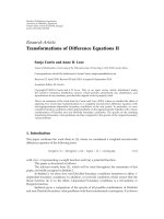
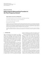
This is illustrated by the following example: consider a
2-channel system (cf. Figure 1) with transmission paths h
1
and h
2
being random 10-taps FIR filters with exponentially
decaying coefficients. To the system white noise is input. Fil-
ter h
1
was adjusted such that the DC response equals 1. With
this example the robustness of blind subspace identification
against order mismatches is assessed under noiseless condi-
tions. Thereto, h
1
and h
2
are identified with the subspace
identification method described in Section 3.4.4,compen-
sating for the ambiguity to allow a fair comparison. Addi-
tionally, the transmission paths are estimated with an NLMS
adaptive filter. In order to check the robustness of both ap-
proaches against order estimate errors, the length of the esti-
mation filters N is changed from 4, 8, and 9 (underestimates)
to 12 (overestimate). The results are plotted in Figure 2.The
solid line corresponds to the frequency response of the 10-
taps filter h
1
. The dashed line shows the frequency response
of the N-taps subspace estimate. The dashed-dotted line rep-
resents the frequency response of the N-taps NLMS estimate.

It was verified that for N
= 10 both methods identify the
correct transmission paths h
1
and h
2
, as predicted by theory.
In the case of a channel-order overestimate (subplot 4), it is
observed that h
1
and h
2
are correctly estimated by the NLMS
approach. Also the subspace algorithm provides correct es-
timates, be it up to a common (filter) factor. This common
factor can be removed using (24). In the case of a channel
order underestimate (subplots 1–3) the NLMS estimates are
clearly superior to those of the subspace method. Whereas
the performance of the adaptive filter gradually deterior ates
with decreasing values of N, the behavior of the subspace
identification method more rapidly deviates from the theo-
retical response.
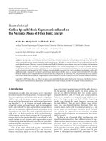
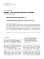
In a second example, a w hite noise signal x is filtered by
two impulse responses h
1
and h
2
of 10 filter taps each. Addi-
tionally, uncorrelated white noise is added to h
1

x and h
2
x
at different signal-to-noise ratios. The system order is esti-
mated based on the singular value spectrum of Y. For this ex-
periment L
= 20 and K = 40. In Figure 3, the 10-logar ithm
of the singular value spectrum is shown for different signal-
to-noise ratios. From (25) it follows that rank
{Y[k]}=29.
In each subplot therefore the 29th singular value is encircled.
Remark that for low, yet realistic sig nal-to-noise ratios such
as 0 dB and 20 dB, there is no clear gap between the signal-
related singular values and the noise-related singular values.
Even when the system order is estimated correctly the sys-
tem estimates

h
1
and

h
2
differ from the true filters h
1
and h
2
.
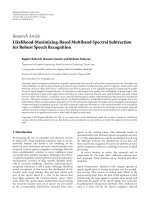
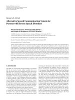
To illustrate this a white noise signal x is filtered by two ran-
dom impulse responses h

1
and h
2
of 20 filter taps each. White
noise is added to h
1
 x and h
2
 x at different signal-to-noise
ratios, leading to y
1
and y
2
.Basedony
1
and y
2
the impulse
responses

h
1
and

h
2
are estimated following (24) and setting
L equal to N.InFigure 4, the angle between h
1
and


h
1
is plot-
ted in degrees as a funct ion of the signal-to-noise ratio. The
angle has been projected onto the first quadrant (0
→ 90
◦
)
as due to the inherent ambiguity, blind subspace algorithms
can solely estimate the orientation of the impulse response
vector, and not the exact amplitude or sign. Observe that the
angle between h
1
and

h
1
is small only at high signal-to-noise
ratios. Remark furthermore that for low signal-to-noise ra-
tios the angle approaches 90
◦
.
3.4.6. Implementation and cost
The dereverberation and the channel estimation procedures
discussed in Sections 3.4.2, 3.4.3,and3.4.4 tend to give rise
to a high algorithmic cost for parameter settings that are typ-
ically used for speech dereverberation. Advanced matrix op-
erations are required, which result in a computational cost of
the order of O(N

3
), where N is the length of the unknown
transmission paths, and a memory storage capacity that is
O(N
2
). This leads to computational and memory require-
ments that exceed the capabilities of many modern computer
systems.
In our simulations the length of the impulse response fil-
ters, that is, N, is computed following (25)withK
= 2N
max
and L = N
max
,whererank{Y[k]} is determined by look-
ing for a gap in the singular value spectrum. In this way,
the impulse response filter length N is restricted to N
max
.
K. Eneman and M. Moonen 7
10
−1
10
0
Frequency amplitude response
00.10.20.30.40.5
Frequency relative to sampling frequency
N
= 4
(a)

10
−1
10
0
Frequency amplitude response
00.10.20.30.40.5
Frequency relative to sampling frequency
N
= 8
(b)
10
−1
10
0
Frequency amplitude response
00.10.20.30.40.5
Frequency relative to sampling frequency
N
= 9
(c)
10
−1
10
0
Frequency amplitude response
00.10.20.30.40.5
Frequency relative to sampling frequency
N
= 12
(d)

Figure 2: Robustness of 2-channel system identification against order estimate errors: 10-taps filters h
1
and h
2
are identified with a blind
subspace identification method and an NLMS adaptive filter. The length of the estimation filters N was changed from 4, 8, and 9 (underesti-
mates) to 12 (overestimate). The solid line corresponds to the f requency response of the 10-taps filter h
1
. The dashed line shows the frequency
response of the N-taps subspace estimate. The dashed-dotted line represents the frequency response of the N-taps NLMS estimate. Whereas
the performance of the adaptive filter gradually deteriorates with decreasing values of N, the behavior of the subspace identification method
more rapidly deviates from the theoretical response.
The impulse responses are computed with the algorithm of
Section 3.4.4,withK
= 5N
max
and L = N. For the computa-
tion of the dereverberation filters, we rely on the zero-forcing
algorithm of Section 3.4.2 with n
= 1andL =N/(M − 1).
Several values have been tried for n, but changing this param-
eter hardly affected the performance of the algorithms. Most
experimentshavebeendonewithN
max
= 100, restricting the
impulse response filter length N to 100. This leads to fairly
small matrix sizes, which however already demand consid-
erable memory consumption and simulation time. To inves-
tigate the effect of larger matrix sizes and hence longer im-
pulse responses, additional simulations have been done with

N
max
= 300. Values of N
max
larger than 300 will quickly lead
to a huge memory consumption and unacceptable simula-
tion times without additionally enhancing the signal (see also
Section 5.1).
3.5. Subband-domain subspace-based
dereverberation
3.5.1. Subband implementation scheme
To overcome the high computational and memory require-
ments of the time-domain subspace approach of Section 3.4,
subband processing can be put forward as an alternative.
In a subband implementation all microphone signals y
m
[k]
8 EURASIP Journal on Audio, Speech, and Music Processing
−0.5
0
0.5
1
1.5
log
10
(σ)
0 10203040
SNR
= 0dB
(a)

−4
−2
0
2
log
10
(σ)
010203040
SNR
= 20 dB
(b)
−4
−2
0
2
log
10
(σ)
010203040
SNR
= 40 dB
(c)
−4
−2
0
2
log
10
(σ)
010203040

SNR
= 60 dB
(d)
Figure 3: Subspace-based system identification: singular value spectrum of the block-Toeplitz data matrix Y at different signal-to-noise
ratios. The system under test is a 9th-order, 2-channel FIR system (N
= 10, M = 2) with white noise input. Additionally, uncorrelated white
noise is added to the microphone signals at different signal-to-noise ratios. Remark that for low, yet realistic signal-to-noise ratios such as
0 dB and 20 dB, there is no clear gap between the signal-related singular values and the noise-related singular values.
are fed into identical analysis filter banks {a
0
, , a
P−1
},as
shown in Figure 5. All subband signals are subsequently
D-fold subsampled. The processed subband signals are
upsampled and recombined in the synthesis filter bank
{s
0
, , s
P−1
}, leading to the system output x. As the chan-
nel estimation and equalization procedure are performed in
the subband domain at a reduced sampling rate, a substantial
cost reduction is expected.
3.5.2. Filter banks
To reduce the amount of overall signal distortion that is in-
troduced by the filter banks and the subsampling, perfect
or nearly perfect reconstruction filter banks are employed
[21, 22]. Oversampled filter banks (P>D) are used to min-
imize the amount of aliasing distortion that is added to the

subband signals during the downsampling. DFT modulated
filter bank schemes are then typically preferred. In many ap-
plications very simple so-called DFT filter banks are used
[22].
3.5.3. Ambiguity elimination
With blind system identification techniques the transmission
paths can only be estimated up to a constant factor. Contrary
to the ful lband approach where a global uncertainty factor α
is encountered (see Section 3.4.4), in a subband implemen-
tation there is an ambiguity factor α
(p)
in each subband.
This leads to significant signal distortion if the ambiguity fac-
tors α
(p)
are not compensated for.
Rahbar et al. [23] proposed a noise robust method to
compensate for the subband-dependent ambiguity that oc-
curs in frequency-domain subspace dereverberation with
1-tap compensation filters. An alternative method is pro-
posed in [20], which can also handle higher-order frequency-
domain compensation filters. These ambiguity elimination
algorithms are quite computationally demanding, as the
eigenvalue or the singular value decomposition has to be
computed of a large matrix. It further appears that the ambi-
guity elimination methods are sensitive to system order mis-
matches.
In the simulations, we apply a frequency-domain sub-
space dereverberation scheme with the DFT-IDFT as anal-
ysis/synthesis filter bank and 1-tap subband models. Further,

P = 512 and D = 256, so that effectively 256-tap time-
domain filters are estimated in the frequency domain. For the
subband channel estimation the blind subspace-based chan-
nel estimation algorithm of Section 3.4.4 is used with N
= 1,
L
= 1, and K = 5. For the dereverberation the zero-forcing
algorithm of Section 3.4.2 is employed with L
= 1andn = 1.
The ambiguity problem that arises in the subband approach
is compensated for based on the technique that is described
in [20]withN
= 256 and P = 512.
K. Eneman and M. Moonen 9
0
10
20
30
40
50
60
70
80
90
Angle between h
1
and

h
1

(degrees)
−100102030405060
Signal-to-noise ratio (dB)
Figure 4: Subspace-based system identification: angle between h
1
and

h
1
as a function of the signal-to-noise ratio for a random 19th-
order, 2-channel system with white noise input (141 realizations are
shown). Uncorrelated white noise is added to the microphone sig-
nals at different signal-to-noise ratios. The angle between h
1
and

h
1
has been projected onto the first quadrant (0 → 90
◦
) as due to the
inherent ambiguity, blind subspace algorithms can solely estimate
the orientation of the impulse response vector, and not the exact
amplitude or sign. Observe that the angle between h
1
and

h
1
is small

only at high signal-to-noise ratios. Remark furthermore that for low
signal-to-noise ratios the angle approaches 90
◦
.
3.5.4. Cost reduction
If there are P subbands that are D-fold subsampled, one may
expect that the transmission path length reduces to N/D in
each subband, lowering the memory storage requirements
from O(N
2
) (see Section 3.4.6)toO(P(N
2
/D
2
)). As typically
P
≈ D, it follows that O(P(N
2
/D
2
)) ≈ O(N
2
/D). As far as
the computational cost is concerned not only the matrix di-
mensions are reduced, also the updating frequency is low-
ered by a factor D, leading to a huge cost reduction from
O(N
3
)toO(P(N
3

/D
4
)) ≈ O(N
3
/D
3
). In practice, however,
the cost reduction is less spectacular, as the transmission path
length will often have to be larger than N/D to appropriately
model the acoustics [24]. Secondly, so far we have neglected
the filter bank cost, which will further reduce the complexity
gain that can be reached with the subband approach. Never-
theless, a significant overall cost reduction can be obtained,
given the O(N
3
) dependency of the algorithm.
Summarizing, the advantages of a subband implemen-
tation are the substantial cost reduction and the decoupled
subband processing, which is expected to give rise to im-
proved performance. The disadvantages are the frequency-
dependent ambiguity, the extra processing delay, as well as
possible signal distortion and aliasing effects caused by the
subsampling [24].
3.6. Frequency-domain subspace-based
matched filtering
In [12] a promising dereverberation algorithm was pre-
sented that relies on 1-dimensional frequency-domain sub-
space tracking. An LMS-type updating scheme was proposed
that offers a low-cost alternative to the matrix-based algo-
rithms of Section 3.4.

The 1-dimensional frequency-domain subspace tracking
algorithm builds upon the following frequency-dependent
data model (compare with (14)) for each frequency f and
each frame n:
y
[n]
( f ) =

h
[n]
1
( f ) ··· h
[n]
M
( f )

T
  
h
[n]
( f )
x
[n]
( f )
+

n
[n]
1
( f ) ··· n

[n]
M
( f )

T
  
n
[n]
( f )
,
(26)
where, for example (similar formulas hold for y
[n]
( f )and
n
[n]
( f )),
x
[n]
( f ) =
P−1

p=0
x[ nP + p]e
− j2π(nP+p) f
(27)
if there is no overlap between frames. If it is assumed that the
transfer functions h
m
[k] ↔ h

m
( f ) slowly vary as a function
of time, h
[n]
( f ) ≈ h( f ).
To dereverberate the microphone signals, equalization
filters e
( f ) have to be computed such that
r
t
( f ) = e
H
( f )h( f ) = 1. (28)
Observe that the matched filter e
( f ) = h( f )/h( f )
2
is a so-
lution to (28).
For the computation of h
( f )ande( f ) the M × M corre-
lation matr ix R
yy
( f ) has to be calculated:
R
yy
( f ) = E

y
[n]
( f )


y
[n]
( f )

H

=
h( f )E



x
[n]
( f )


2

h
H
( f )
  
R
xx
( f )
+ E

n
[n]

( f )

n
[n]
( f )

H


 
R
nn
( f )
,
(29)
where it is assumed that the speech and noise components
are uncorrelated. It is seen from (29) that the speech correla-
tion matrix R
xx
( f ) is a rank-1 matrix. The noise correlation
matrix R
nn
( f ) can be measured during speech pauses.
The transfer function vector h
( f )canbeestimatedus-
ing the generalized eigenvalue decomposition (GEVD) of the
correlation matrices R
yy
( f )andR
nn

( f ),
R
yy
( f ) = Q( f )Σ
y
( f )Q
H
( f )
R
nn
( f ) = Q( f )Σ
n
( f )Q
H
( f )
(30)
10 EURASIP Journal on Audio, Speech, and Music Processing
x
h
1
y
1
a
0
.
.
.
y
(a
0

)
1
D
y
(0)
1
e
(0)
1
.
.
.
+
D
s
0
.
.
.
a
P−1
y
(a
P−1
)
1
D
y
(P−1)
1

e
(0)
M
+
h
M
y
M
.
.
.
.
.
.
a
0
y
(a
0
)
M
D
y
(0)
M
e
(P−1)
1
.
.

.
D
.
.
.
s
P−1
.
.
.
y
(a
P−1
)
M
a
P−1
D
y
(P−1)
M
e
(P−1)
M
x
+
Figure 5: Multi-channel subband dereverberation system: the microphone signals y
m
are fed into identical analysis filter banks {a
0

, , a
P−1
},
and are subsequently D-fold subsampled. After processing the subband signals are upsampled and recombined in the synthesis filter bank
{s
0
, , s
P−1
}, leading to the system output x.
with Q( f ) an invertible, but not necessarily orthogonal ma-
trix [25]. As the speech correlation matrix
R
xx
( f ) = R
yy
( f ) − R
nn
( f ) = Q( f )

Σ
y
( f ) − Σ
n
( f )

Q
H
( f )
(31)
hasrank1,itisequaltoR

xx
( f ) = σ
2
x
( f )q
1
( f )q
H
1
( f )with
q
1
( f ) the pr incipal generalized eigenvector corresponding to
the largest generalized eigenvalue. Since
R
xx
( f ) = σ
2
x
( f )q
1
( f )q
H
1
( f ) = E



x
[n]

( f )


2

h( f )h
H
( f ),
(32)
h
( f ) can be estimated up to a phase shift e
jθ( f )
as

h( f ) = e
jθ( f )
h( f ) =


h( f )




q
1
( f )


q

1
( f )e
jθ( f )
(33)
if
h( f ) is known. It is assumed that the human auditory
system is not very sensitive to this phase shift.
If the additive noise is spatially white, R
nn
( f ) = σ
2
n
I
M
and
then h
( f ) can be estimated as the principal eigenvector cor-
responding to the largest eigenvalue of R
yy
( f ). It is this algo-
rithmic variant, which assumes spatially white additive noise,
that was originally proposed in [12].
Using the matched filter
e
( f ) =

h( f )


h( f )



2
=
q
1
( f )


q
1
( f )




h( f )


, (34)
the dereverberated speech signal
x
[n]
( f )isfoundas
x
[n]
( f ) = e
H
( f )y
[n]

( f )
= e
− jθ( f )
x
[n]
( f )+
q
H
1
( f )


q
1
( f )




h( f )


n
[n]
( f ),
(35)
from wh ich the time-domain signal
x[ k]canbecomputed.
As can be seen from (34), the norm β
=h( f ) has to

be known in order to compute e
( f ). Hence, β has to be mea-
sured beforehand, which is unpractical, or has to be fixed to
an environment-independent constant, for example, β
= 1,
as proposed in [12].
The algorithm is expected to fail to dereverberate the
speech signal if β is not known or is wrongly estimated, as
in a matched filtering approach mainly the filtering with the
inverse of
h( f )
2
is responsible for the dereverberation (see
also Section 3.4.2). Hence, we could claim that the method
proposed in [12] is primarily a noise reduction algorithm
and that the dereverberation problem is not t ruly solved.
If the frequency-domain subspace estimation algorithm
is combined with the ambiguity elimination algorithm pre-
sented in Section 3.5.3, the transmission paths h
m
( f )can
be determined up to within a global scaling factor. Hence,
β
=h( f ) can be computed and does not have to be known
in advance. Uncertainties on β,however,whicharedueto
the limited precision of the channel estimation procedure
and the “lag error” of the algori thm during tracking of time-
varying transmission paths, affect the performance of the
subspace tracking algorithm.
In our simulations, we compare two versions of the

subspace-based matched filtering approach, both relying on
the eigenvalue decomposition of R
yy
( f ). One variant uses
β
= 1 and the other computes β as described in Section 3.5.3.
For all implementations the block length is set equal to 64,
N
= 256, and the FFT size P = 512. To evaluate the algo-
rithm under ideal conditions we simulate a batch version in-
stead of the LMS-like tracking variant of the algorithm pro-
posed in [12].
4. EVALUATION CRITERIA
The performance of the dereverberation algorithms pre-
sented in Sections 3.1 to 3.6 has been assessed through a
number of experiments that are described in Section 5.For
the evaluation, two performance indices have been applied
and the ability of the algor ithms to enhance the word recog-
nition rate of a speech recognition system has been deter-
mined. In this section, the automatic speech recognition sys-
tem is described and the performance indices are defined that
have been used throughout the evaluation.
K. Eneman and M. Moonen 11
4.1. Performance indices
For a proper comparison between the different dereverbera-
tion procedures, we consider two performance indices, which
will be referred to as δ
1
and δ
2

. They can be derived from the
totalresponsefilter
r
t
=
M

m=1
e
m
 h
m
, (36)
where r
t
describes the total response from the source signal x
to the output
x if the compensator C is linear (see Figure 1).
Let r
t
( f ) be the frequency response of r
t
, then δ
1
is defined
as
δ
1
=
μ

|r
t
|
σ
|r
t
|
(37)
with
μ
|r
t
|
=

1/2
−(1/2)


r
t
( f )


df ,
σ
2
|r
t
|

=

1/2
−(1/2)



r
t
( f )


−
μ
|r
t
|

2
df.
(38)
In the case of perfect dereverberation, the total response filter
r
t
is a delay, and hence |r
t
( f )| is flat. Therefore, with a l arger
δ
1
, more dereverberation is expected. This relative standard

deviation measure only takes into account the amplitude of
the frequency response of r
t
and neglects the phase response.
A more exact measure can be defined in the time domain.
If r
t
can be represented as an Lth-order FIR filter
r
t
=

r
t
[0] ··· r
t
[L]

T
, (39)
performance index δ
2
is defined as
δ
2
=
r
max
t



r
t


, (40)
where
r
max
t
= max
n=0:L



r
t
[n]



. (41)
Here, a unique maximum is assumed, for conciseness.
Hence, δ
2
2
corresponds to the energy in the dominant im-
pulse of r
t
divided by the total energy in r

t
. Again, with a
larger δ
2
, m ore dereverberation is expected. It is easily veri-
fied that 0 <δ
2
≤ 1.
The first part of the evaluation that is presented in this
paper relies on simulated impulse responses h
m
[26]. Hence,
the total response filter can be computed following (36). The
second part of the evaluation is based on experiments with
recorded real-life data. In that case, the transmission paths
h
1
···h
M
,andsor
t
, are unknown, hence the proposed per-
formance indices cannot be applied. However, in the absence
of any knowledge about the transmission paths, the total re-
sponse filter can still be computed based on x and
x,provided
that x is known. The impulse responses then are measured
offline by inputting white noise to the system and then ap-
plying an NLMS adaptive filter.
Note that in the definition of the performance indices

δ
1
and δ
2
, it is implicitly assumed that the dereverberation
algorithm is linear, and therefore can be described by lin-
ear dereverberation filters e
1
···e
M
, as shown in Figure 1.
Cepstrum-based dereverberation techniques are inherently
nonlinear. They can hence not be described by linear derever-
beration filters. Performance indices δ
1
and δ
2
are therefore
not defined for the cepstrum-based approach.
4.2. Automatic speech recognition
Object ive quality measures to check dereverberation perfor-
mance are difficult to identify. Apart from the two perfor-
mance indices defined in Section 4.1, in this paper we rely
on the recognition rate of an automatic speech recognizer
to compare different algorithms. One of the possible tar-
get applications of dereverberation software is indeed speech
recognition. Automatic speech recognition systems are typi-
cally trained under more or less anechoic conditions. Recog-
nition rates therefore drop whenever signals are applied that
are recorded in a moderately or highly reverberant envi-

ronment. In order to enhance the speech recognition rate,
dereverberation software can be used as a preprocessing step
to reduce the amount of reverberation that is input to the
speech recognition system. In this way, increased recognition
rates are hoped for. In this paper, the effect of reverberation
on the performance of the speech recognizer is measured and
several dereverberation algorithms are evaluated as a means
to enhance the recognition rate.
For the recognition experiments [27], a speaker-
independent large vocabulary continuous speech recognition
system was used that has been developed at the ESAT-PSI re-
search group of Katholieke Universiteit Leuven, Belgium. In
this system, the data is sampled at 16 kHz and is first pre-
emphasized. Then, every 10 milliseconds, the power spec-
trum is computed using a window with a time horizon of 30
milliseconds. By means of a nonlinear mel-scaled triangular
filterbank, 24 mel-spectrum coefficients are computed and
transformed to the log domain. By subtracting the average,
the coefficients are mean normalized. In this way, robustness
is added against differences in the recording channel. A fea-
ture vector with 72 parameters is then constructed by com-
bining the 24 coefficients with their first and second time
derivatives. The feature vector is reduced in size and decor-
related, as explained in [28, 29]. A more detailed overview of
the acoustic modeling can be found in [27, 30]. The search
module is described in [31].
The data set that was used for the speech recognition
experiments is the Wall Street Journal November 92 speech
recognition evaluation test set [27]. It consists of 330 sen-
tences, amounting to about 33 minutes of speech, uttered by

eight different speakers, both male and female. The (clean)
data set is recorded at 16 kHz and contains almost no ad-
ditive noise, nor reverberation. With the recognition system
described in the previous paragraph a word error rate (WER)
12 EURASIP Journal on Audio, Speech, and Music Processing
Table 1: A list of the dereverberation algorithms that have been experimentally evaluated, as presented in Section 5. References are given to
previous sections and to the literature, as well as indicative relative complexity numbers for each of the algorithms.
no. Algorithm Used graphical symbol Discussed in section
Reference to the
literature
Relative algorithmic
complexity
Unprocessed microphone signal  ———
(1) Delay-and-sum beamforming  Section 3.1 [11, 17]1.0
(2) Unnormalized matched filtering  Section 3.2 [17]2.7
(3) Cepstrum-based dereverberation
∗ Section 3.3 [2] 52.7
(4)
Zero-forcing time-domain
subspace-based dereverberation
 Sections 3.4.2, 3.4.4, 3.4.5
[20]
121.6
(5)
Zero-forcing frequency-domain
subspace-based dereverberation
 Section 3.5
[20]
192.3
(6)

Matched filtering subspace-based
dereverberation, β
= 1
 Section 3.6
[12]
14.8
(7)
Matched filtering subspace-based
dereverberation, β computed
× Sections 3.6, 3.5.3
[12, 20]
223.1
of 1.9% can be obtained on the clean Wall Street Journal
benchmark test set.
It is important to note that the speech recognizer is
trained on the clean, noise-free, unreverberated data, and
that the recognition system does not dispose of any special
features to combat additive noise or reverberation. Hence,
the improvements in word error rate that are observed dur-
ing simulation are entirely due to the preprocessing signal
enhancement tools that are added to the system. Better word
error r ates may possibly be obtained if the recognizer was
trained on noisy or reverberated data. However, the noise
and reverbera tion that are added during training may not
correspond to the actual noise and reverberation that are ob-
served when the recognizer is used afterwards to recognize
unknown speech fragments in real environments. It is not
clear whether a system trained on typical noises and rever-
beration would do better than a recognizer trained on clean
speech. Furthermore, most pr actical speech recognition sys-

tems, for which the recognizer used in this paper serves as a
reference, are trained on clean data. If they are used in voice-
controlled systems operating in noisy and reverberated en-
vironments, performance decreases are expected similar to
those observed in our experiments.
5. EXPERIMENTAL RESULTS
For the evaluation the three criteria are taken into account
that have been presented in Sections 4.1 and 4.2. Most of the
experiments have been carried out under stationary acous-
tics and are based on data that was generated in a simulated
acoustic environment using the method described in [26]. In
all the experiments omnidirectional microphones were used,
placed on a linear array, 5 cm apart. The speaker was in front
of the array in the broadside direction (making an angle of
90
◦
with the array). The sampling frequency used through-
out the simulations is 16 kHz.
In total 7 dereverberation algorithms have been com-
pared, as summarized in Table 1. The table gives references
to the literature and to previous sections in the text, and
an indication of the relative complexity of the algorithms.
The exact parameter setting can be found at the end of the
sections mentioned in the third column of the table. The
complexity numbers are based on the execution t ime of the
current implementation of the algorithms. So far, the algo-
rithms have been mainly evaluated and optimized towards
dereverberation performance. The implementation schemes
still need to be improved.
5.1. Reverberation time

A first parameter that has a strong influence on the perfor-
mance of the algorithms is the reverberation time. The rever-
beration time T
60
is defined as the time needed for the sound
energy to fall by 60 dB [16]. Typical reverberation times are
of the order of hundreds or even thousands of milliseconds.
For a typical office room T
60
is between 100 and 400 millisec-
onds, while for a church T
60
can be several seconds.
The simulated recording room is rectangular (36 m
3
)and
empty, with all wal ls having the same energy reflection co-
efficient ρ. Hence, the reverberation time can be computed
using Eyring’s formula [16]:
T
60
=
0.163V
−S log
e
ρ
, (42)
where S is the total surface of the room and V is the volume
of the room.
The results corresponding to the first experiment are

presentedinFigures6 and 7, showing performance indices
δ
1
or δ
2
and the word error rate as a function of the re-
verberation time T
60
. Recall that higher δ
1
or δ
2
values,
or lower word error rates correspond to smaller expected
residual reverberation. A number of T
60
-values were con-
sidered that are representative for low-reverberant up to
office room environments, ranging from 64, 87, 155, 199,
274, 319, 422 to 533 milliseconds. All room environments
have been generated using the method described in [26].
K. Eneman and M. Moonen 13
0
0.5
1
1.5
2
2.5
3
3.5

4
4.5
5
Performance index δ
1
0.10.15 0.20.25 0.30.35 0.40.45 0.5
Reverberation time T
60
(seconds)
Reverberated microphone signal
Delay-and-sum beamforming
Unnormalized matched filtering
Zero-forcing time-domain subspace-based dereverb. (N
= 100)
Zero-forcing frequency-domain subspace-based dereverberation
Matched filtering subspace-based dereverberation, β
= 1
Matched filtering subspace-based dereverberation, β computed
Zero-forcing time-domain subspace-based dereverb. (N
= 300)
(a)
0.1
0.2
0.3
0.4
0.5
0.6
0.7
0.8
0.9

1
Performance index δ
2
0.10.15 0.20.25 0.30.35 0.40.45 0.5
Reverberation time T
60
(seconds)
Reverberated microphone signal
Delay-and-sum beamforming
Unnormalized matched filtering
Zero-forcing time-domain subspace-based dereverb. (N
= 100)
Zero-forcing frequency-domain subspace-based dereverberation
Matched filtering subspace-based dereverberation, β
= 1
Matched filtering subspace-based dereverberation, β computed
Zero-forcing time-domain subspace-based dereverb. (N
= 300)
(b)
Figure 6: Performance indices δ
1
and δ
2
as a function of the reverberation time: only the beamforming algorithm and the unnormalized
matched filter succeed in enhancing the signal quality. The subspace-based approaches fail to improve the signal quality.
0
10
20
30
40

50
60
70
80
90
100
Word e rror r ate (%)
0.10.20.30.40.5
Reverberation time T
60
(seconds)
Reverberated microphone signal
Cepstrum-based dereverberation
Delay-and-sum beamforming
Unnormalized matched filtering
Matched filtering subspace-based dereverberation, β
= 1
Figure 7: Word error rate as a function of the reverberation time:
apparently, the speech recognition system shows a significant per-
formance loss in highly reverberant rooms. Only the beamform-
ing algorithm, the cepstrum-based dereverber a tion and the unnor-
malized matched filter succeed in enhancing the signal quality. The
subspace-based approaches fail to improve the signal quality.
The reverberation times were computed following (42).
Also the direct-to-reverberant ratios were calculated corre-
sponding to the considered T
60
values, resulting in drr =
6.16, 4.19, 0.8, −0.59, −2.24, −3.01, −4.37, and −5.48 dB, re-
spectively. The direct-to-reverberant ratio was computed fol-

lowing [32] as the energy in the direct path impulse to the
third microphone divided by the energy in the rest of the
acoustic impulse response to the third microphone. During
all simulations the distance between the speaker and the cen-
ter of the 6-microphone array was 94 cm.
The reference curve (thick full line) corresponds to the
nonenhanced, reverberated signals. It is seen from Figure 7
that the speech recognition system shows a significant perfor-
mance loss in more highly reverberant rooms. This justifies
the need for adequate dereverberation of the input signals.
It can furthermore be observed that only the beamforming
algorithm, the cepstrum-based dereverberation, and the un-
normalized matched filter are able to enhance the signals and
show better per formance than the unprocessed reference, es-
pecially for large reverberation times.
Apparently, the subspace-based dereverberation algo-
rithms fail to enhance the signals, unfortunately. Increas-
ing N
max
(compare the time-domain subspace approach with
N
max
= N = 100 and N
max
= N = 300) will t ypically not im-
prove the signal enhancement, and only put higher demands
on the computational and memory capabilities of the com-
puter system. The reason why subspace algor ithms fail to en-
hance the signals is that they are typically “blind” and hence
estimate the transmission paths based on the microphone

signals only. The first algorithmic step consists in estimat-
ing the order of the transmission path filters. Given the fact
that speech signals are nonpersistently exciting and that the
system order is typically high (even infinite in fact), the or-
der of the transmission path filters is always underestimated.
This results in large errors as subspace algorithms are highly
sensitive to system-order mismatches (see Figure 2).
The above observations that follow from Figures 6 and 7
have also been confirmed through subjective listening tests:
the cepstrum and the beamforming approach clearly reduce
14 EURASIP Journal on Audio, Speech, and Music Processing
0
0.5
1
1.5
2
2.5
3
3.5
4
4.5
5
Performance index δ
1
23456
Number of microphones
Reverberated microphone signal
Delay-and-sum beamforming
Unnormalized matched filtering
Zero-forcing time-domain subspace-based dereverb. (N

= 100)
Zero-forcing frequency-domain subspace-based dereverberation
Matched filtering subspace-based dereverberation, β
= 1
Matched filtering subspace-based dereverberation, β computed
(a)
0.1
0.2
0.3
0.4
0.5
0.6
0.7
0.8
0.9
1
Performance index δ
2
23456
Number of microphones
Reverberated microphone signal
Delay-and-sum beamforming
Unnormalized matched filtering
Zero-forcing time-domain subspace-based dereverb. (N
= 100)
Zero-forcing frequency-domain subspace-based dereverberation
Matched filtering subspace-based dereverberation, β
= 1
Matched filtering subspace-based dereverberation, β computed
(b)

Figure 8: Performance indices δ
1
and δ
2
as a function of the number of microphones: the performance of the algorithms only marginally
improves if the number of m icrophones is increased. Beamforming and standard unnormalized matched filtering are able to remove some
of the reverberation.
0
5
10
15
20
25
30
35
40
45
50
Word e rror r ate (%)
23456
Number of microphones
Reverberated microphone signal
Cepstrum-based dereverberation
Delay-and-sum beamforming
Unnormalized matched filtering
Matched filtering subspace-based dereverberation, β
= 1
Figure 9: Word error rate as a function of the number of micro-
phones: the performance of the algorithms only marginally im-
proves if the number of microphones is increased. Beamform-

ing, cepstrum-based dereverberation, and standard unnormalized
matched filtering succeed in removing some of the reverberation.
that amount of dereverberation, whereas the subspace al-
gorithms do not improve or sometime worsen the signal
quality. The unnormalized matched filtering algorithm leaves
a considerable amount of residual reverberation, which is
confirmed by the word error rate score and by performance
index δ
1
, but contradicted by the high score on the δ
2
index.
5.2. Number of microphones
The number of microphones was gradually increased from 2
to 6. The distance between the speaker and the center of the
microphone array was again 94 cm. The reflection coefficient
was chosen such that the reverberation time (see (42)) corre-
sponded to 274 milliseconds. The other characteristics of the
room were left unchanged. The results are shown in Figures
8 and 9. It appears that beamforming, cepstrum-based dere-
verberation, and standard unnormalized matched filtering
areabletoremovesomeofthereverberation.Unfortunately,
subspace algorithms do not seem to be able to enhance the
reverberated signals. It is furthermore observed that if the
number of microphones is increased, the performance of the
algorithms only marginally improves. This performance in-
crease is possibly due to the increased number of degrees of
freedom and the increased spatial sampling that is obtained
when more microphones are involved.
5.3. Distance between speaker and microphone array

The distance d between the speaker and the center of
the 6-microphone array was changed between 70.7 cm to
4.93 m. The other characteristics of the room were left un-
changed. Hence, the reverberation time T
60
(see (42)) re-
mained fixed to 274 milliseconds. Based on the results that
are presented in Figures 10 and 11 it can be concluded
that, again, beamforming, standard unnormalized matched
filtering, and cepstrum-based dereverberation outperform
the unprocessed reverberated signal. We should keep in
mind, however, that the unnormalized matched filtering al-
gorithm uses a priori knowledge. Hence, a performance loss
K. Eneman and M. Moonen 15
0
0.5
1
1.5
2
2.5
3
3.5
4
Performance index δ
1
11.522.533.544.5
Distance between speaker and microphone array (m)
Reverberated microphone signal
Delay-and-sum beamforming
Unnormalized matched filtering

Zero-forcing time-domain subspace-based dereverb. (N
= 100)
Zero-forcing frequency-domain subspace-based dereverberation
Matched filtering subspace-based dereverberation, β
= 1
Matched filtering subspace-based dereverberation, β computed
(a)
0
0.1
0.2
0.3
0.4
0.5
0.6
0.7
0.8
0.9
1
Performance index δ
2
11.522.533.544.5
Distance between speaker and microphone array (m)
Reverberated microphone signal
Delay-and-sum beamforming
Unnormalized matched filtering
Zero-forcing time-domain subspace-based dereverb. (N
= 100)
Zero-forcing frequency-domain subspace-based dereverberation
Matched filtering subspace-based dereverberation, β
= 1

Matched filtering subspace-based dereverberation, β computed
(b)
Figure 10: Performance indices δ
1
and δ
2
as a function of the distance between speaker and microphone array: beamforming and standard
unnormalized matched filtering outperform the unprocessed reverberated signal and the subspace technique. Performance decreases with
increasing speaker-to-array distance.
0
10
20
30
40
50
60
70
80
90
100
Word e rror r ate (%)
11.522.533.544.5
Distance between speaker and microphone array (m)
Reverberated microphone signal
Cepstrum-based dereverberation
Delay-and-sum beamforming
Unnormalized matched filtering
Matched filtering subspace-based dereverberation, β
= 1
Figure 11: Word error rate as a function of the distance between

speaker and microphone array: beamforming, standard unnormal-
ized matched filtering and cepstrum-based dereverberation outper-
form the unprocessed reverberated signal and the subspace tech-
nique. Performance decreases with increasing speaker-to-array dis-
tance.
is expected if the transmission paths h
m
(see Figure 1)areun-
known and have to be estimated.
Note that the dereverberation performance decreases
with increasing speaker-to-array distance. A reason for this
could be that less direct sound is captured when the speaker
is far from the array. The relative amount of late reflec-
tions, also called reverberation, then increases and a more
complex reverberation scenario is obtained. To quantify
this, the direct-to-reverberant ratio was calculated follow-
ing [32] for each of the scenarios we considered, that is,
for d
= 0.707, 0.94, 1.87, 2.65, 4.93 meter, resulting in drr =
−
0.12, −2.24, −7.70, −10.69, −10.11 dB, respectively.
5.4. Additive noise
Finally, noise has been added to the multichannel speech
recordings at different signal-to-noise ratios (SNR). For the
computation of the SNR, first speech and noise periods are
determined. Then the unbiased SNR can be computed as the
mean variance of the speech signal during speech periods di-
vided by the mean variance of the noise. White noise as well
as speech-weighted noise have been added to the reverber-
ated speech signals. In order to obtain a desired SNR level,

the noise amplitude was adjusted on the first data base sig-
nal. For simplicity, equal-noise amplitudes were then applied
to the other data base signals. In order to validate the spa-
tial selectivity properties of the dereverberation algorithms
both uncorrelated noise and spatially correlated noise have
been considered. In all cases, the number of microphones
was fixed to 6. The speaker was rig ht in front of the array
at a distance of 94 cm from the center of the microphone
array. The reflection coefficients of the room were chosen
such that the reverberation time (see (42)) corresponded to
274 milliseconds. The other characteristics of the room were
left unchanged with respect to the previous experiments. To
generate spatially correlated noise a noise source was posi-
tioned in the recording room at 146 cm from the center of
16 EURASIP Journal on Audio, Speech, and Music Processing
0
10
20
30
40
50
60
70
80
90
100
Word e rror r ate (%)
5 101520 25303540
SNR (dB)
Microphone signal (noise, no reverberation)

Microphone signal (noise + reverberation)
Cepstrum-based dereverberation
Delay-and-sum beamforming
Unnormalized matched filtering
Matched filtering subspace-based dereverberation, β
= 1
Figure 12: Word error rate as a function of the SNR for uncorre-
lated additive white noise: the speech recognizer shows a significant
performance decrease in n oisy, reverberated environments. Observe
that the effect of the noise on the overall performance of the al-
gorithms is significant for SNR levels lower than 20 dB. Best per-
formance is obtained with beamforming, standard unnormalized
matched filtering, and cepstrum-based dereverberation. Finally, a
performance increase is observed for the subspace techniques at low
SNR levels.
the microphone, at an angle of 38 degrees with respect to
the main axis of the array. In this way, the distance between
the noise source and the speaker was 175 cm. The impulse
responses were computed to each of the microphones us-
ing the method described in [26]. The noise signal was then
convolved with these impulse responses and added to the
speech components at each microphone.
The word error rate is shown as a function of the SNR
in Figures 12, 13, 14 for each noise configuration. It can be
concluded that the effect of the noise on the overall perfor-
mance of the algorithms is significant for SNR levels lower
than 20 dB. Apparently, the type of noise (white, speech-
weighted) as such does not play an impor tant role. Best per-
formance is obtained with beamforming, standard unnor-
malized matched filtering, and cepstrum-based dereverber-

ation. Finally, it is observed that subspace techniques show a
performance increase at low SNR levels. Maybe this is due to
the fact that at low SNR levels we see the effect of the noise
reduction rather than that of the dereverberation capabilities
of the subspace algorithms.
Remark that we also added noise to the clean data base
signals (i.e., signals without reverberation) under the same
signal-to-noise ratio as in the case of the reverberated mul-
tichannel data. The corresponding results are labeled “noise,
no reverberation.” The main objective was to determine the
performance of the speech recognizer on the additive noise-
only data and to compare it with data to which additive noise
as well as reverberation were added. It can be concluded that
0
20
40
60
80
100
Word e rror r ate (%)
5 1015202530
SNR (dB)
Microphone signal (noise, no reverberation)
Microphone signal (noise + reverberation)
Cepstrum-based dereverberation
Delay-and-sum beamforming
Unnormalized matched filtering
Matched filtering subspace-based dereverberation, β
= 1
Figure 13: Word error rate as a function of the SNR for spatially

correlated additive white noise: the speech recognizer shows a sig-
nificant performance decrease in noisy, reverberated environments.
Observe that the effect of the noise on the overall performance of
the algorithms is significant for SNR levels lower than 20 dB. Best
performance is obtained with beamforming, standard unnormal-
ized matched filtering, and cepstrum-based dereverberation.
adding only additive noise only mildly increases the word er-
ror rate. Hence, we conclude that reverberation has a more
negative impact on the overall recognition rate than additive
noise.
5.5. Real-life recordings
Next, also some real-life experiments were performed. The
corresponding results can be found in Ta ble 2. The real-life
data was recorded in the speech labor atory (68.5 m
3
) of the
Electrotechnical Department of the Katholieke Universiteit
Leuven, Belgium. The speaker was imitated by a loudspeaker
in order to preserve stationary a coustics. The acoustic im-
pulse responses from the speaker to each of the 6 micro-
phones was determined (for experiment 2 and 4) with an
NLMS adaptive filter based on white noise data. The reflec-
tivity of the room was changed over the four experiments and
the reverberation time T
60
was computed using Schroeder’s
method, a reference to which can be found in [26]. Observe
that in the fourth experiment spatially correlated speech-
weighted noise was added at about 8 dB SNR. The position
of the noise source was similar to that of the simulated envi-

ronment of Section 5.4 and Figure 14.
Proper dereverberation is only obtained with beam-
forming and cepstrum-based dereverberation. Unnormal-
ized matched filtering appears to be effective only if both
reverberation and noise are added. The effectiveness of the
dereverberation algorithms also appears to be smaller than
K. Eneman and M. Moonen 17
Table 2: Dereverberation performance on real-life experiments. For each of the algorithms the word error rate (WER) is shown. Proper
dereverberation is only obtained with beamforming and cepstrum-based dereverberation. Unnormalized matched filtering appears to be
effective only if both reverberation and noise are added. The effectiveness of the dereverberation algorithms also appears to be smaller than
with simulated data.
Experiment 1234
Speaker-to-array distance (m) 1.87 1.85 1.87 1.32
Reverberation time T
60
(ms) 121 244 275 293
Signal-to-noise ratio (dB) — — — 7.87
WER WER WER WER
Unprocessed microphone signal 6.35% 14.09% 16.79% 49.97%
Cepstrum-based dereverber ation 5.98% 13.64% 13.95% 42.39%
Delay-and-sum beamforming 6.20% 14.63% 15.34% 36.99%
Unnormalized matched filtering — 24.92% — 44.70%
Zero-forcing frequency-domain subspace — 20.53% — 75.70%
Matched filtering subspace, β
= 1 10.01% 21.37% 25.42% 56.55%
0
20
40
60
80

100
Word e rror r ate (%)
0 5 10 15 20 25 30
SNR (dB)
Microphone signal (noise, no reverberation)
Microphone signal (noise + reverberation)
Cepstrum-based dereverberation
Delay-and-sum beamforming
Unnormalized matched filtering
Matched filtering subspace-based dereverberation, β
= 1
Figure 14: Word error rate as a function of the SNR for spatially
correlated additive speech-weighted noise: the speech recognizer
shows a significant performance decrease in noisy, reverberated en-
vironments. Observe that the effect of the noise on the overall per-
formance of the algorithms is significant for SNR levels lower than
20 dB. Best performance is obtained with beamforming, standard
unnormalized matched filtering, and cepstrum-based dereverbera-
tion.
with simulated data. It is observed from Table 2 that 26%
relative improvement can be obtained (see experiment 4) if
both reverberation and noise are added. In the cases where
no noise was present, the relative improvement is limited
to 17%.
Of all algorithms that have been evaluated through the
experiments presented in Section 5, standard techniques
such as beamforming and the cepstrum-based approach
seem most effective in combating reverberation distortion.
More recently proposed techniques such as the subspace
methods discussed in Sections 3.4, 3.5,and3.6 fail to enhance

the signal quality, despite the larger computational complex-
ity and memory requirements. Apart from limitations due to
the undermodeling discussed in Sec tion 3.4.5, the algorithms
also suffer from the time variations of the acoustics, which
are common in practice. This furthermore complicates the
identification task. More simple, classical solutions such as
beamforming and cepstrum-based techniques do not require
a modeling and tracking of the acoustics, and are hence much
more robust against these time variations.
Hence, most signal enhancement systems that are cur-
rently used in speech communication applications such as
teleconferencing, handsfree telephony, and voice-controlled
systems mainly concentrate on the suppression of back-
ground noise and acoustic echoes, and simply deal with
reverberation by assuming relatively small speaker-to-
microphone distances or by applying simple, classical dere-
verberation algorithms such as beamforming and cepstrum-
based techniques. As long as these systems are used in lowly
to moderately reverberating environments with the speaker
at a close distance to the microphones, good performance is
expected. Whenever the environment is highly reverberating
and the speaker-to-microphone distance is large, severely re-
verberated speech is expected, which can considerably com-
promise sp eech intelligibility.
6. CONCLUSIONS
Dereverberation algorithms are employed to preserve the sig-
nal quality in speech communication systems. Several clas-
sical and more recently developed multichannel dereverber-
ation algorithms have been compared. It was shown that
classical solutions, such as beamforming, cepstral derever-

beration, and unnormalized matched filtering show mod-
erate performance increases w ith respect to the process-
ing of nonenhanced, reverberated speech signals. More ad-
vanced subspace-based dereverberation techniques, on the
other hand, did not provide any signal enhancement despite
18 EURASIP Journal on Audio, Speech, and Music Processing
their high-computational load. There are mainly three im-
pediments that explain this poor performance. First of all,
blind subspace methods are highly sensitive to model or-
der mismatches. The effect of this is most prominent for
higher-order systems, which are commonly encountered in
speech enhancement applications. Secondly, the quality of
the model is compromised by the additive noise that is super-
imposed on the signals. Subspace techniques are known to be
quite sensitive to small amounts of additive noise. Thirdly, in
a real-life situations, the acoustics are time varying, and need
to be tracked, which makes it even more difficult to obtain a
reliable system model. Subspace-based identification proce-
dures furthermore tend to give rise to a high algorithmic cost
and large memory consumption for parameter settings that
are typically used in speech applications. In practice, very of-
ten the model order needs to be limited for computational
reasons. Better performance might be reached if higher, and
hence more realistic model orders can be applied. This would
be feasible if cheaper implementation schemes were avail-
able.
List of symbols
Lower case bold-faced letters are used to denote vectors and
upper case bold-faced letters to denote matrices. In addition
the following notation is used throughout the paper:

 Convolution operation
F Fourier transform
x[ k] Discrete-time-domain signal x
x
( f ) Frequency-domain representation of x[k]
x
rc
[m] Real cepstrum of x[k]
A
T
Transpose of A
A
∗
Complex conjugate of A
A
†
Pseudo-inverse of A
A
H
Hermitian transpose of A
1 Vector with all elements equal to 1
0 Zero matrix
0
N
N × N zero matrix
0
M×N
M × N zero matrix
I
N

N × N identity matrix
· 2-norm of a vector or a matrix
Other notation is explained in the text.
ACKNOWLEDGMENTS
The authors would like to thank Dr. Jacques Duchateau for
making available the automatic speech recognition system of
the ESAT-PSI research group. This research work was car-
ried out at the ESAT Laboratory of the Katholieke Univer-
siteit Leuven, in the frame of the Belgian State Interuniver-
sity Poles of Attraction Programmes P5/22 and P5/11. The
scientific responsibility is assumed by its authors.
REFERENCES
[1] D.Bees,M.Blostein,andP.Kabal,“Reverberantspeechen-
hancement using cepstral processing,” in Proceedings of IEEE
International Conference on Acoustics, Speech, and Signal Pro-
cessing (ICASSP ’91), vol. 2, pp. 977–980, Toronto, Ontario,
Canada, May 1991.
[2] Q G. Liu, B. Champagne, and P. Kabal, “A microphone array
processing technique for speech enhancement in a reverber-
ant space,” Speech Communication, vol. 18, no. 4, pp. 317–334,
1996.
[3] A. Oppenheim and R. Schafer, Digital Signal Processing, chap-
ter 10, Prentice-Hall, Englewood Cliffs, NJ, USA, 1975.
[4] A. P. Petropulu and S. Subramaniam, “Cepstrum based decon-
volution for speech dereverberation,” in Proceedings of IEEE
International Conference on Acoustics, Speech, and Signal Pro-
cessing (ICASSP ’94), vol. 1, pp. 9–12, Adelaide, Australia,
April 1994.
[5] J. B. Allen, D. A. Berkley, and J. Blauert, “Multimicrophone
signal-processing technique to remove room reverberation

from speech signals,” TheJournaloftheAcousticalSocietyof
America, vol. 62, no. 4, pp. 912–915, 1977.
[6] T. Wittkop and V. Hohmann, “Strategy-selective noise reduc-
tion for binaural digital hearing aids,” Speech Communication,
vol. 39, no. 1-2, pp. 111–138, 2003.
[7] M. Miyoshi and Y. Kaneda, “Inverse filtering of room acous-
tics,” IEEE Transactions on Acoustics, Speech, and Signal Pro-
cessing, vol. 36, no. 2, pp. 145–152, 1988.
[8] P. A. Nelson, F. Orduna-Bustamante, and H. Hamada, “Inverse
filter design and equalization zones in multichannel sound re-
production,” IEEE Transactions on Speech and Audio Process-
ing, vol. 3, no. 3, pp. 185–192, 1995.
[9] Y. Grenier, “A microphone array for car environments,” Speech
Communication, vol. 12, no. 1, pp. 25–39, 1993.
[10] C. Sydow, “Broadband beamforming for a microphone array,”
The Journal of the Acoustical Society of America, vol. 96, no. 2,
pp. 845–849, 1994.
[11] B. D. van Veen and K. M. Buckley, “Beamforming: a versa-
tile approach to spatial filtering,” IEEE ASSP Magazine, vol. 5,
no. 2, pp. 4–24, 1988.
[12] S. Affes and Y. Grenier, “A signal subspace tracking algorithm
for microphone array processing of speech,” IEEE Transactions
on Speech and Audio Processing, vol. 5, no. 5, pp. 425–437,
1997.
[13] E. Moulines, P. Duhamel, J F. Cardoso, and S. Mayrargue,
“Subspace methods for the blind identification of multichan-
nel FIR filters,” IEEE Transactions on Signal Processing, vol. 43,
no. 2, pp. 516–525, 1995.
[14] A J. van der Veen, S. Talwar, and A. Paulraj, “Blind identifica-
tion of FIR channels carrying multiple finite alphabet signals,”

in Proceedings of IEEE International Conference on Acoustics,
Speech, and Signal Processing (ICASSP ’95), vol. 2, pp. 1213–
1216, Detroit, Mich, USA, May 1995.
[15] S. Gannot and M. Moonen, “Subspace methods for multi-
microphone speech dereverberation,” in Proceedings of the 7th
IEEE/EURASIP International Workshop on Ac oustic Echo and
Noise Control (IWAENC ’01), pp. 47–50, Darmstadt, Germany,
September 2001.
[16] H. Kuttruff, Room Acoustics, Applied Science Publishers, Essex,
England, 2nd edition, 1979.
[17] D. Johnson and D. Dudgeon, Array Signal Processing, Prentice-
Hall, Englewood Cliffs, NJ, USA, 1993.
K. Eneman and M. Moonen 19
[18]D.vanGerven,S.vanCompernolle,P.Wauters,W.Ver-
straeten, K. Eneman, and K. Delaet, “Multiple beam broad-
band beamforming: filter design and real-time implementa-
tion,” in Proceedings of IEEE Workshop on Applications of Signal
Processing to Audio and Acoustics (WASPAA ’95), pp. 173–176,
New Paltz, NY, USA, October 1995.
[19] G. B. Giannakis and S. D. Halford, “Blind fractionally spaced
equalization of noisy FIR channels: direct and adaptive solu-
tions,” IEEE Transactions on Signal Processing, vol. 45, no. 9,
pp. 2277–2292, 1997.
[20] K. Eneman and M. Moonen, “Ambiguity elimination in
frequency-domain subspace identification,” Internal Report
ESAT-SCD 06.151, p. 12, Katholieke Universiteit Leuven,
Leuven, Belgium, 2007, https://gilber t.med.kuleuven.be/
∼koen/reports/06-151.pdf.
[21] K. Eneman and M. Moonen, “DFT modulated filter bank
design for oversampled subband systems,” Signal Processing,

vol. 81, no. 9, pp. 1947–1973, 2001.
[22] P. Vaidyanathan, Multirate Systems and Filter Banks, Prentice-
Hall, Englewood Cliffs, NJ, USA, 1993.
[23]K.Rahbar,J.P.Reilly,andJ.H.Manton,“Afrequencydo-
main approach to blind identification of MIMO FIR systems
driven by quasi-stationary signals,” in Proceedings of IEEE In-
ternational Conference on Acoustics, Speech, and Signal Process-
ing (ICASSP ’02), vol. 2, pp. 1717–1720, Orlando, Fla, USA,
May 2002.
[24] K. Eneman and M. Moonen, “Hybrid subband/frequency-
domain adaptive systems,” Signal Processing,vol.81,no.1,pp.
117–136, 2001.
[25] S. Doclo and M. Moonen, “Combined frequency-domain
dereverberation and noise reduction technique for multi-
microphone speech enhancement,” in Proceedings of the 7th
IEEE/EURASIP International Workshop on Ac oustic Echo and
Noise Control (IWAENC ’01), pp. 31–34, Darmstadt, Germany,
September 2001.
[26] J. B. Allen and D. A. Berkley, “Image method for efficiently
simulating small-room acoustics,” TheJournaloftheAcoustical
Society of America, vol. 65, no. 4, pp. 943–950, 1979.
[27] K. Eneman, J. Duchateau, M. Moonen, D. van Compernolle,
and H. van Hamme, “Assessment of dereverberation algo-
rithms for large vocabulary speech recognition systems,” in
Proceedings of the 8th European Conference on Speech Com-
munication and Technology (Eurospeech ’03), pp. 2689–2692,
Geneva, Switzerland, September 2003.
[28] J. Duchateau, K. Demuynck, D. van Compernolle, and P.
Wambacq, “Class definition in discriminant feature analysis,”
in Proceedings of the 7th European Conference on Speech Com-

munication and Technology (Eurospeech ’01), vol. 3, pp. 1621–
1624, Aalborg, Denmark, September 2001.
[29] K. Demuynck, J. Duchateau, D. van Compernolle, and P.
Wambacq, “Improved feature decorrelation for HMM-based
speech recognition,” in Proceedings of the 5th International
Conference on Spoken Language Processing (ICSLP ’98), vol. 7,
pp. 2907–2910, Sydney, Australia, November-December 1998.
[30] J. Duchateau, K. Demuynck, and D. van Compernolle,
“Fast and accurate acoustic modelling with semi-continuous
HMMs,” Speech Communication, vol. 24, no. 1, pp. 5–17, 1998.
[31] K. Demuynck, J. Duchateau, D. van Compernolle, and P.
Wambacq, “An efficient search space representation for large
vocabulary continuous speech recognition,” Speech Commu-
nication, vol. 30, no. 1, pp. 37–53, 2000.
[32] D. Bees, Enhancement of acoustically reverberant speech using
cepstral methods, Ph.D. thesis, McGill University, Montreal,
Canada, July 1990.