Báo cáo hóa học: " Research Article 4D Near-Field Source Localization Using Cumulant" ppt

Hindawi Publishing Corporation
EURASIP Journal on Advances in Signal Processing
Volume 2007, Article ID 17820, 10 pages
doi:10.1155/2007/17820
Research Article
4D Near-Field Source Localization Using Cumulant
Junli Liang,
1, 2
Shuyuan Yang,
1, 2
Junying Zhang,
3
Li Gao,
1, 2
and Feng Zhao
4
1
Institute of Acoustics, Chinese Academy of Sciences, Beijing 100080, China
2
Graduate School of Chinese Academy of Sciences, Beijing 100039, China
3
National Laboratory of Radar Signal Processing, Xidian University, Xi’an 710071, China
4
School of Computer Science and Engineering, Xidian University, Xi’an 710071, China
Received 20 September 2006; Revised 1 January 2007; Accepted 24 March 2007
Recommended by Sabine Van Huffel
This paper proposes a new cumulant-based algorithm to jointly estimate four-dimensional (4D) source parameters of multiple
near-field narrowband sources. Firstly, this approach proposes a new cross-array, and constructs five high-dimensional Toeplitz
matrices using the fourth-order cumulants of some properly chosen sensor outputs; secondly, it forms a parallel factor (PARAFAC)
model in the cumulant domain using these matrices, and analyzes the unique low-rank decomposition of this model; thirdly, it
jointly estimates the frequency, two-dimensional (2D) directions-of-arrival (DOAs), and range of each near-field source from the

matrices via the low-rank three-way array (TWA) decomposition. In comparison with some available methods, the proposed algo-
rithm, which efficiently makes use of the array aperture, can localize N
− 3 sources using N sensors. In addition, it requires neither
pairing parameters nor multidimensional search. Simulation results are presented to validate the performance of the proposed
method.
Copyright © 2007 Junli Liang et al. This is an open access article distributed under the Creative Commons Attribution License,
which permits unrestricted use, distribution, and reproduction in any medium, provided the original work is properly cited.
1. INTRODUCTION
Estimation of directions-of-arrival (DOAs) has received a
significant amount of attention over the last several decades.
It is a key problem in array signal processing areas such
as radar, sonar, radio astronomy, and mobile communica-
tion systems. Many classical algorithms have been devel-
oped to solve this problem, such as the maximum likelihood
(ML) method [1], the MUSIC method [2], and the ESPRIT
method [3]. Most of these methods make the assumption
that the sources are located relatively far from the array so
that the waves emitted by these sources can be considered as
plane waves. With such an assumption, each signal wavefront
can be characterized by the DOAs of the source [4]. However,
when a source is located close to the array (i.e., near field)
[5], the wavefront must be characterized by both the DOAs
and the range parameters of the source. A good approxima-
tion of the nonlinear propagation delay function consists of
its second-order Taylor expansion (Fresnel approximation).
Using such an approximation, the propagation delay varies
quadratically with sensor location, and the range informa-
tion must be incorporated into the signal model. Therefore,
the estimation of the near-field source parameters is more
complicated than that of far-field one, and the classical DOAs

estimation methods for far-field sources are no longer appli-
cable.
To solve near-field source localization problem, many al-
gorithms were addressed, such as the ML method [5], the 2D
MUSIC methods [6–9], the linear prediction methods [10,
11], and the ESPRIT-like methods [12–15]. However, these
methods for near-field source localization [5–15] mainly fo-
cused on two-dimensional (2D) case, that is, estimating the
azimuth and range only. Recently, several algorithms [16–
18] were addressed to deal with three-dimensional (3D)
source localization, which is a joint azimuth, elevation, and
range estimation problem. For example, Kabaoglu et al. [16]
proposed an expectation-maximization (EM)-based algo-
rithm, in which only a subset of the parameters is esti-
mated iteratively while the other parameters remain fixed.
Despite its effectiveness, this algorithm has extremely de-
manding computational complexity due to the search com-
putation and iteration process. Hung et al. [17]extended
the 2D MUSIC method to 3D one, but this method re-
quires a 3D search of the extended cost function. To avoid
these search computations, a second-order statistics (SOS)-
based algorithm was addressed recently in [18], but this
2 EURASIP Journal on Advances in Signal Processing
method, which suffers a heavy loss of the array aperture,
canlocalizenotmorethan(1/4)(N
− 5) sources using N
sensors. In addition, it requires a quadratic phase trans-
form algorithm to pair the separately estimated par ame-
ters. Note that all these algorithms addressed in [16–18]
cannot estimate signal frequencies simultaneously. However,

when these frequencies need to be estimated, the 3D near-
field source localization problem actually becomes a four-
dimensional (4D) one. Hence it is necessary to develop
a joint 4D parameter estimation algorithm for near-field
sources.
The above-mentioned analyses show that the main diffi-
culties of near-field source localization problem consist of: (i)
avoiding multidimensional search which results in extremely
demanding computational complexity; (ii) reducing the loss
of the array ap erture; (iii) pairing source parameters (i.e., fre-
quency, azimuth, elevation, and range) so as to localize the
near-field sources accurately.
As a useful analysis tool of data arr ays, the parallel factor
(PARAFAC) model [19–22] is a generalization of low-rank
matrix decomposition to three-way arrays (TWAs) or multi-
way arrays (MWAs). Unlike singular value decomposition,
PARAFAC does not impose orthogonality constraints, and
relies on certain conditions [23–29] regarding the unique-
ness of low-rank TWA (or MWA) decomposition. Because
of its direct link to low-rank decomposition, PARAFAC has
wide applications in numerous and diverse disciplines [22,
26, 30, 31].
In this paper, we develop a new cumulant-based algo-
rithm for 4D near-field source localization (see [32] for the
detailed definition of cumulant). The key point of this pa-
per is to construct five high-dimensional Toeplitz matrices
using the cumulants of some properly chosen sensor out-
puts and form an identifiable PARAFAC model in the fourth-
order cumulant domain. The proposed algorithm requires
neither pairing parameters nor multidimensional search. In

addition, it can efficiently use the array aperture.
The rest of this paper is organized as follows. The sig-
nal and PARAFAC models are introduced in Section 2.A
4D near-field source localization algorithm is developed in
Section 3. Simulation results are presented in Section 4.Con-
clusions are drawn in Section 5.
2. PROBLEM FORMULATION AND PARAFAC MODEL
2.1. Problem formulation
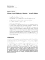
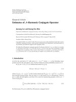
Consider L near-field, narrowband, and independent radiat-
ing sources impinging upon a cross array aligned with x and
y axes, as shown in Figure 1. Each subarray consists of uni-
formly spaced omnidirectional sensors with inter-element
spacing d.Thex subarray consists of 2N sensors, while the
y subarray is composed of 3 ones. The cross one is chosen
as the phase reference point. After being down-converted to
baseband and sampled at a proper sampling rate that sat-
isfies the Nyquist rate, the signals received by the (i,0)th
and (0, m)th sensors can be approximately expressed by (see
[14, 18] for details):
x
i,0
(k) =
L

l=1
s
l
(k)e
jω
l

k
e
j(iγ
xl
+i
2
φ
xl
)
+ n
i,0
(k),
i =−N +1, , −1, 0, 1, , N,
x
0,m
(k) =
L

l=1
s
l
(k)e
jω
l
k
e
j(mγ
yl
+m
2

φ
yl
)
+ n
0,m
(k),
m
=−1, 1,
(1)
respectively, where s
l
(k)e
jω
l
k
denotes the lth source signal
with the normalized radian frequency ω
l
, while n
i,0
(k)and
n
0,m
(k) represent the additive measurement noise. In addi-
tion, electric angles γ
xl
, φ
xl
, γ
yl

,andφ
yl
are given by
γ
xl
=−
2πdsin α
l
cos β
l
λ
,
φ
xl
=
πd
2

1 − sin
2
α
l
cos
2
β
l

λr
l
,

γ
yl
=−
2πdsin α
l
sin β
l
λ
,
φ
yl
=
πd
2

1 − sin
2
α
l
sin
2
β
l

λr
l
,
(2)
for l
= 1, , L,respectively,whereλ is the related propa-

gation wavelength, and
{α
l
, β
l
, r
l
} denote the azimuth, eleva-
tion, and range of the lth source.
The objective of this paper is to jointly estimate the fre-
quency ω
l
, the 2D DOA {α
l
, β
l
}, and the range r
l
of the lth
source for l
= 1, , L.
Throughout the rest of the paper, the following hypothe-
ses are assumed to hold.
(H1) The source signals are statistically mutually indepen-
dent, non-Gaussian, and narrowband stationary pro-
cesses with nonzero kurtosis.
(H2) The sensor noise is zero-mean Gaussian signal and in-
dependent of the source signals.
(H3) The source parameters are different from each other,
that is, γ

xi
+φ
xi
/= γ
xj
+φ
xj
, γ
xi
−φ
xi
/= γ
xj
−φ
xj
, γ
yi
−φ
yi
/=
γ
yj
− φ
yj
, γ
yi
+ φ
yi
/= γ
yj

+ φ
yj
,andω
i
/= ω
j
for i/= j.In
fact, this hypothesis can be alleviated, and the detailed
analyses are given in Section 3.
(H4) For uniquely identifying L sources, we require d
≤ λ/4
and L<2N.
2.2. PARAFAC model [22, 26, 30]
Definition 1. Consider a (I × J × K)-dimensional TWA X =
(R ⊗ U)W
T
(⊗ stands for Kronecker product) with typical
element x
i, j,k
and the F-component trilinear decomposition
x
i, j,k
=
F

f =1
r
i, f
u
j, f

w
k, f
(3)
Junli Liang et al. 3
(−N +1,0)(−N +2,0) (−1, 0) (0, 0) (1, 0)
(0, 1)
(N − 1, 0) (N,0)
(0,
−1)
x
z
y
lth near-field source
r
l
α
l
β
l
······
Figure 1: proposed cross-array for 4D near-field source localization problem.
for all i = 1, , I, j = 1, , J,andk = 1, , K,wherer
i, f
represents the (i, f )th element of (I × F)-dimensional ma-
trix R. Similarly, u
j, f
and w
k, f
stand for ( j, f )th and (k, f )th
elements of (J

× F)and(K × F)-dimensional matrices U and
W,respectively.Equation(3) expresses x
i, j,k
as a sum of F
rank-1 triple products; it is known as PARAFAC analysis of
x
i, j,k
.
Definition 2. Let g
i
(R) denote a diagonal matrix composed of
the ith row of matrix R,andg
−1
(Λ) stands for a row vector
made up of the diagonal elements of diagonal matrix Λ.
In a compact form, X can be expressed in terms of its 2D
slice X
i
((J × K)-dimensional matrix, that is, X
i
= [x
i,:,:
]) as
X
i
= Ug
i
(R)W
T
, i = 1, , I. (4)

Under certain conditions, X can be decomposed uniquely
into matrices R, U,andW. These conditions are based on
the notion of Kruskal-rank [23–26].
Definition 3. The Kruskal rank (or k-rank) [23–26]ofmatrix
R is k
R
if and only if arbitrary k
R
columns of R are linearly
independent and either R has k
R
columns or R contains a set
of k
R
+ 1 linearly dependent columns. Note that Kruskal rank
is always less than or equal to the conventional matrix r a nk.
If R is of full column rank, then it is also of full k-rank.
Theorem 1. Let X
i
be defined as in (4). R, U,andW can be
recovered uniquely up to permutation and scaling ambiguity,
irrespective of whether the eleme nts of X are real values [23–
25] or complex ones [26], as long as
k
R
+ k
U
+ k
W
≥ 2F +2, (5)

which is the well-known Kr uskal’s condit ion. In fact, the re are
different results that guarantee PARAFAC uniqueness under
different conditions [27–29]. For instance, Leurgans et al. [27]
analyzed the condition for the decomposition of three-way ar-
rays which have rank 1. While Lathauwer [29] considered the
decomposition of higher-order tens ors which have the property
that the rank is smaller than the greatest dimension.
3. PROPOSED ALGORITHM
3.1. PARAFAC model formulation
To develop a new joint estimation algorithm, we begin with
the (2N
×2N)-dimensional cumulant matrix C
1
, the (m, n)th
element of which has the following form:
C
1
(m, n) =
L

l=1
c
4sl
e
j(γ
xl
+φ
xl
)
e

j(m−n)(γ
xl
+φ
xl
)
,1≤ m, n ≤ 2N,
(6)
where c
4s
l
= cum(s
k
(k), s
∗
l
(k), s
l
(k), s
∗
l
(k)) is the fourth-
order kurtosis of the lth source. Note that C
1
can be rep-
resented in a compact form as C
1
= AΩΛC
4s
A
H

,where
the superscript H denotes the Hermitian transpose, C
4s
=
diag[c
4s
1
, c
4s
2
, , c
4s
L
], Ω = diag[e
jγ
x1
, e
jγ
x2
, , e
jγ
xL
], Λ =
diag[e
jφ
x1
, e
jφ
x2
, , e

jφ
xL
], A = [
a
1
a
2
··· a
L
], and a
l
=
[1, e
j(γ
xl
+φ
xl
)
, , e
j(2N−1)(γ
xl
+φ
xl
)
]
T
, l = 1, , L.
Due to the complicated signal model of near-field
sources, it is difficult to derive such a cumulant matrix from
the array outputs directly. However, it is easily seen from (6)

that the matrix C
1
has the same structure as Toeplitz matrices
theoretically. It is well known that Toeplitz matrices are ma-
trices having constant entries along their diagonals. Hence
we consider approximating C
1
by virtue of a set of estimated
cumulants.
For different sensor lags, we define a column vector h
1
,
the ith element of which can be represented as
h
1
(i,1)= cum

x
0,0
(k), x
∗
0,0
(k), x
(N+1)−i,0
(k), x
∗
−
N+i,0
(k)


=
L

l=1
c
4s
l
e
j(2N−2i)(γ
xl
+φ
xl
)
e
j(γ
xl
+φ
xl
)
, i = 1, 2, ,2N,
(7)
where the superscript
∗ denotes the complex conjugate. It is
obvious that the elements of h
1
can merely “fill” the (m, n)th
position of an approximated matrix, where (m
−n)isaneven
4 EURASIP Journal on Advances in Signal Processing
number. To construct the whole approximated matrix, we

define another column vector h
2
h
2
(i,1)= cum

x
1,0
(k), x
∗
0,0
(k), x
(N+1)−i,0
(k), x
∗
−N+i,0
(k)

=
L

l=1
c
4s
l
e
j(2N−2i+1)(γ
xl
+φ
xl

)
e
j(γ
xl
+φ
xl
)
, i = 1, 2, ,2N,
(8)
which can complement the rest of the approximated matrix.
Furthermore, for different sensor and time lags, we define
other eight column vectors:
h
3
(i,1)= cum

x
0,0
(k), x
∗
−
1,0
(k), x
(N+1)−i,0
(k), x
∗
−
N+i,0
(k)


=
L

l=1
c
4s
l
e
j(2N−2i)(γ
xl
+φ
xl
)
e
j2γ
xl
, i = 1, 2, ,2N,
h
4
(i,1)= cum

x
1,0
(k), x
∗
−
1,0
(k), x
(N+1)−i,0
(k), x

∗
−N+i,0
(k)

=
L

l=1
c
4s
l
e
j(2N−2i+1)(γ
xl
+φ
xl
)
e
j2γ
xl
, i = 1, 2, ,2N,
h
5
(i,1)= cum

x
0,0
(k +1),x
∗
0,0

(k), x
(N+1)−i,0
(k), x
∗
−
N+i,0
(k)

=
L

l=1
c
4s
l
e
j(2N−2i)(γ
xl
+φ
xl
)
e
j(γ
xl
+φ
xl
)
e
jω
l

,
i
= 1, 2, ,2N,
h
6
(i,1)= cum

x
1,0
(k +1),x
∗
0,0
(k), x
(N+1)−i,0
(k), x
∗
−
N+i,0
(k)

=
L

l=1
c
4s
l
e
j(2N−2i+1)(γ
xl

+φ
xl
)
e
j(γ
xl
+φ
xl
)
e
jω
l
,
i
= 1, 2, ,2N,
h
7
(i,1)= cum

x
0,0
(k), x
∗
0,−1
(k), x
(N+1)−i,0
(k), x
∗
−
N+i,0

(k)

=
L

l=1
c
4s
l
e
j(2N−2i)(γ
xl
+φ
xl
)
e
j(γ
xl
+φ
xl
)
e
j(γ
yl
−φ
yl
)
,
i
= 1, 2, ,2N,

h
8
(i,1)= cum

x
1,0
(k), x
∗
0,−1
(k), x
(N+1)−i,0
(k), x
∗
−N+i,0
(k)

=
L

l=1
c
4s
l
e
j(2N−2i+1)(γ
xl
+φ
xl
)
e

j(γ
xl
+φ
xl
)
e
j(γ
yl
−φ
yl
)
,
i
= 1, 2, ,2N,
h
9
(i,1)= cum

x
0,0
(k), x
∗
0,1
(k), x
(N+1)−i,0
(k), x
∗
−N+i,0
(k)


=
L

l=1
c
4s
l
e
j(2N−2i)(γ
xl
+φ
xl
)
e
j(γ
xl
+φ
xl
)
e
j(−γ
yl
−φ
yl
)
,
i
= 1, 2, ,2N,
h
10

(i,1)= cum

x
1,0
(k), x
∗
0,1
(k), x
(N+1)−i,0
(k), x
∗
−
N+i,0
(k)

=
L

l=1
c
4s
l
e
j(2N−2i+1)(γ
xl
+φ
xl
)
e
j(γ

xl
+φ
xl
)
e
j(−γ
yl
−φ
yl
)
,
i
= 1, 2, ,2N.
(9)
Thus, by virtue of these eight column vectors, we can con-
struct four Toeplitz matricesC
2
, C
3
, C
4
,andC
5
:
C
i
(m, n)
=
⎧
⎪

⎪
⎪
⎨
⎪
⎪
⎪
⎩
h
2×i

N −
m − n − 1
2
,1

if (m−n)isanoddnumber,
h
2×i−1

N −
m − n
2
,1

if (m−n)isanevennumber,
1
≤ m, n ≤ 2N, i = 2, ,5.
(10)
It is obvious that these matrices have the following compact
forms:

C
2
= AΩ
2
C
4s
A
H
,
C
3
∼
=
AΩΛΦ
1
C
4s
A
H
,
C
4
= AΩΛΦ
2
C
4s
A
H
,
C

5
= AΩΛΦ
3
C
4s
A
H
,
(11)
where
Φ
1
= diag

e
jω
1
, e
jω
2
, , e
jω
L

,
Φ
2
= diag

e

j(γ
y1
−φ
y1
)
, e
j(γ
y2
−φ
y2
)
, , e
j(γ
yL
−φ
yL
)

,
Φ
3
= diag

e
j(−γ
y1
−φ
y1
)
, e

j(−γ
y2
−φ
y2
)
, , e
j(−γ
yL
−φ
yL
)

.
(12)
Since all the source signals are assumed to have nonzero kur-
tosis, C
4s
is an invertible diagonal matrix. Besides, because
of the assumptions γ
xi
+ φ
xi
/= γ
xj
+ φ
xj
and L ≤ 2N (see
Section 2.1), A is a Vandermonde matrix with full column
rank L.Hence,C
1

, C
2
, C
3
, C
4
,andC
5
are all (2N × 2N)-
dimensional matrices with rank L.
In fact, since the snapshot size is finite, the estimates

C
1
,

C
2
,

C
3
,

C
4
,and

C
5

contain some estimation errors, which can
form other five matrices, that is, V
1
, V
2
, V
3
, V
4
,andV
5
.Sim-
ilar to (4), we define a (2N
× 2N × 5)-dimensional TWA

X,
the five 2D slices ((2N
× 2N)-dimensional matrix) of which
can be represented as

X
1
=

C
1
= AΩΛC
4s
A
H

+ V
1
,

X
2
=

C
2
= AΩ
2
C
4s
A
H
+ V
2
,

X
3
=

C
3
= AΩΛΦ
1
C
4s

A
H
+ V
3
,

X
4
=

C
4
= AΩΛΦ
2
C
4s
A
H
+ V
4
,

X
5
=

C
5
= AΩΛΦ
3

C
4s
A
H
+ V
5
.
(13)
Note that

X can be represented in a compact form as

X = (R ⊗ U)W
T
+ V = X + V, (14)
where both X and V are (2N
× 2N × 5)-dimensional TWAs,
X
= (R ⊗ U)W
T
,andV consists of V
1
, V
2
, V
3
, V
4
,andV
5

.
Junli Liang et al. 5
In addition, W = A
∗
, U = A,and
R
=
⎡
⎢
⎢
⎢
⎢
⎢
⎣
g
−1

ΩΛC
4s

g
−1

Ω
2
C
4s

g
−1


ΩΛΦ
1
C
4s

g
−1

ΩΛΦ
2
C
4s

g
−1

ΩΛΦ
3
C
4s

⎤
⎥
⎥
⎥
⎥
⎥
⎦
. (15)

It can be seen that the hypothesis (H3) in Section 2.1
can enable X to certainly meet Theorem 1. In fact, this de-
manding hypothesis can be alleviated so that this theorem
still holds under the following general assumption. Assume
these two hypotheses to hold: (i) to any two sources, γ
xi
+φ
xi
/=
γ
xj
+ φ
xj
for i/= j; (ii) not less than two sources have either
different ω
i
,ordifferent γ
xi
− φ
xi
,ordifferent γ
yi
− φ
yi
,or
different γ
yi
+ φ
yi
. Note that the first hypothesis can guaran-

tee that k
W
= L and k
U
= L, while the second one ensures
k
R
≥ 2, and thus X still satisfies Theorem 1 under this gen-
eral assumption. In fact, this result holds for one source case,
that is, L
= 1, irrespective of these two hypotheses, as long
as X does not contain an identically zero 2D slice along any
dimension [22, 26]. In the actual implementation, X is ap-
proximated by

X.
3.2. Description of the proposed algorithm
As one of the methods for fitting PARAFAC model, trilin-
ear alternating least s quare (TALS) approach [26, 30, 31, 33–
36] (other methods [37–39] also can be used to deal with
this fitting problem, such as the TALAE method proposed in
[37]) is appealing primarily because it is guaranteed to con-
verge monotonically but also because of its relative simplicity
(no parameter to tune, and each step solves a standard least
square problem) and good performance [22, 35]. In addi-
tion, this method also allows easy incorporation of weighted
loss function, missing values, and constraints on some or all
of the factors [22, 36]. The basic idea behind this method for
PARAFAC model fitting is to update a subset of parameters
using least squares regression every time while keeping the

other previous parameter estimates fixed. Such an alternat-
ing projections-type procedure is iterated for all subsets of
parameters until the convergence is achieved. The computa-
tional complexity per iteration [26, 31] is equal to the cost of
computing a matrix pseudoinverse, that is, O(F
3
+ IJKF),
where I, J, K,andF are defined in Section 2.2. Note that
when F is small relative to I, J,andK,onlyafewiterations
are usually required to achieve convergence.
In this paper, we use the COMFAC algorithm [26, 33, 34]
to fit the PARAFAC model. This algorithm is essentially a fast
implementation of TALS, and speeds up the least squares fit-
ting procedure by working with a compressed version of the
data, thereby avoiding brute-force implementation of alter-
nating least square in the raw data space. It consists of three
main parts: (i) compression; (ii) initialization and fitting of
PARAFAC in compressed space; (iii) decompression and re-
finement in the raw data space. The COMFAC MATLAB
function described in [34]hassuchaform[R, U, W,
•, i] =
comfac(

X, f , •, •, •, •), where inputs

X and f ,respectively,
stand for the decomposing TWA and the corresponding
factor number (in this paper, it represents the source num-
ber), while outputs
{R, U, W} and i represent the iden-

tification results (matrices) and the iteration number re-
quired for the low-rank decomposition. In addition,
• denote
some other options (see [34] for details). Thus the proposed
method can be described as follows.
Step 1. Estimate the cumulant matrices

C
1
,

C
2
,

C
3
,

C
4
,and

C
5
, then construct TWA

X.
Step 2. Implement the COMFAC MATLAB function [R, U,
W,

•, i] = comfac(

X, f , •, •, •, •) to fit the PARAFAC model

X, and get the estimates

R,

U,and

W.
Step 3. The estimates of e
j(γ
xl
+φ
xl
)
, e
j(γ
xl
−φ
xl
)
, e
j(−γ
yl
−φ
yl
)
,

e
j(γ
yl
−φ
yl
)
,andω
l
can be obtained from

R,

U,and

W:
η
1,l
= e
j(γ
xl
+

φ
xl
)
=
1
2(2N − 1)

2N−1


i=1

U(i +1,l)

U(i, l)
+
2N−1

i=1

W
∗
(i +1,l)

W
∗
(i, l)

,
η
2,l
= e
j(γ
xl
−

φ
xl
)

=

R(2, l)

R(1, l)
,
η
3,l
= e
j(γ
yl
−

φ
yl
)
=

R(4, l)

R(1, l)
,
η
4,l
= e
j(−γ
yl
−

φ

yl
)
=

R(5, l)

R(1, l)
,
(16)
ω
l
= ∠


R(3, l)

R(1, l)

, (17)
for l
= 1, , L,respectively.
Step 4. From (16), we can obtain the estimates of
{γ
xl
, γ
yl
,
φ
xl
}:

γ
xl
=
∠

η
1,l
η
2,l

2
,

φ
xl
=
∠

η
1,l
/η
2,l

2
,
γ
yl
=
∠


η
3,l
/η
4,l

2
.
(18)
Step 5. Thus, we can obtain the estimates of
{α
l
, β
l
} and r
l
:
α
l
= asin

λ
2πd

γ
2
xl
+ γ
2
yl


,

β
l
= atan


γ
yl
γ
xl

,
r
l
=
πd
2
λ

φ
xl

1 − sin
2
α
l
cos
2


β
l

,
(19)
for l
= 1, , L,respectively.
6 EURASIP Journal on Advances in Signal Processing
Since matrix estimates

R,

U,and

W are simultaneously
obtained from the low-rank decomposition of

X, and their
respective elements, which come from the columns with the
same sequence number, are the functions of the parameters
of the same source, the proposed algorithm avoids extra pair-
ing computation. However, the method addressed in [18]
needs to decompose each matrix respectively, and thus re-
quires a complicated quadratic phase transform method to
pair the separately estimated parameters.
Since it can construct five (2N
× 2N)-dimensional ma-
trices using 2N + 2 sensors, our algorithm can localize
2N
− 1 sources. However, the method developed in [18]can

construct six ([(1/2)(N +1)]
× [(1/2)(N + 1)])-dimensional
matrices using 2N + 3 sensors (since the algorithm in [18]
has a symmetric cross array configuration, we arrange such
acrossarrayof2N + 3 sensors for this algorithm), and can
localize not more than (1/2)(N
− 1) sources. Regarding the
main computational complexity, we only consider the mul-
tiplications involved in calculating the matrices and in per-
forming the low-rank TWA decomposition (or the matrix
eigendecomposition in [18]). The method in [18]requires
calculating four (N + 1)-dimensional vectors to construct
six ([(1/2)(N +1)]
× [(1/2)(N + 1)])-dimensional SOS ma-
trices, so it requires O
{4(N +1)m}.However,ouralgorithm
requires calculating ten 2N-dimensional cumulant vectors
to construct five (2N
× 2N)-dimensional Toeplitz matri-
ces, so it requires O
{180 Nm}. Relative to the computational
complexity from the matrix decomposition (or the low-
rank TWA decomposition in our algorithm), the method
in [18] decomposes two ([(3/2)(N +1)]
× [(1/2)(N + 1)])-
dimensional matrices separately, so it requires O
{(9/8)(N +
1)
3
} and our algorithm uses the COMFAC algorithm to fit

a(2N
× 2N × 5)-dimensional TWA, and thus the computa-
tional complexity per iteration is O
{L
3
+20N
2
L}. For the sim-
ulations in Section 4, only 2 iterations are required to achieve
convergence. Hence the total computational complexity of
our algorithm is O
{180 Nm +2(L
3
+20N
2
L)}, and is larger
than that of [18](i.e.,O
{4(N +1)m +(9/8)(N +1)
3
}) in the
case of m
 N,wherem,2N +2,andL stand for the snap-
shot, sensor, and source number, respectively.
4. SIMULATION RESULTS
Some simulations are conducted in this section to assess the
proposed algorithm. We consider a 12-element cross array
with element spacing d
= (λ/4), as shown in Figure 1.Two
equal-power, statistically independent narrow-band sources
(bandwidth

= 25 kHz), respectively with center frequency 2.0
and 2.5 MHz, radiate on the cross array. The sampling rate is
20 MHz and the received signals are polluted by zero-mean
additive white Gaussian noises. The two sources are located
at
{α
1
= 5
◦
, β
1
= 30
◦
, r
1
= 1.5λ} and {α
2
= 50
◦
, β
2
=
15
◦
, r
2
= 0.3λ}, respectively. For comparison, we simultane-
ously execute the algorithm in [18] which assumes the fre-
quencies are known. Since the algorithm in [18] uses a sym-
metric cross array, we arrange such an array of 13 s ensors

for this algorithm. The DOAs, frequency, and range estimates
are scaled in units of rad, rad/s, and wavelength, respectively,
20151050
SNR (dB)
−80
−70
−60
−50
−40
−30
−20
−10
0
MSE (dB)
1st source, our algorithm
2nd source, our algorithm
1st source, CRB
2nd source, CRB
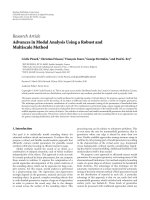
Figure 2: Estimation MSE of the frequencies versus input SNR.
and the performance of these algorithms is measured by the
mean-square error (MSE) of the estimated parameters. 200
independent Monte Carlo runs are performed to evaluate the
estimation errors. At the same time the Cramer-Rao bounds
(CRB) for estimating source parameters are obtained from
the inverse of Fisher information matrix [1], and shown in
the relevant figures.
For the following exper iments, we use the short ver-
sion [R, U , W,
•, i] = comfac(


X,2) of COMFAC algorithm
[33, 34] to fit the (10
× 10 × 5)-dimensional TWA. In the
COMFAC algorithm, we implement the initialization using
DTLD function, and employ data compression using the
Tucker3 three-way model [40, 41]. For these simulations,
only 2 iterations are required to achieve convergence.
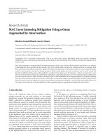
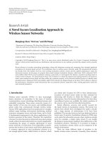
In the first experiment, the effect of signal-to-noise
(SNR) on the performance of the proposed algorithm is in-
vestigated. The snapshot number is set equal to 400, and the
SNR varies from 0 dB to 20 dB. Figures 2, 3, 4,and5 show
the MSE of the frequency, azimuth, elevation, and range es-
timates of the two sources, respectively.
In the second experiment, the influence of snapshot
number on the performance of the proposed algorithm is in-
vestigated. The SNR is set equal to 10 dB, and the snapshot
number varies from 200 to 2000. Figures 6, 7, 8,and9 show
the MSE of the frequency, azimuth, elevation, and range es-
timates of the two sources, respectively.
From these simulations, we can arrive at the following
conclusion.
(i) Our algor ithm has a satisfactory frequency estimation
accuracy even at low SNR region, while that of [18]
is based on the assumption that the frequencies are
known.
Junli Liang et al. 7
20151050
SNR (dB)
−60
−50

−40
−30
−20
−10
0
10
20
MSE (dB)
1st source, our algorithm
2nd source, our algorithm
1st source, [18]
2nd source, [18]
1st source, CRB
2nd source, CRB
Figure 3: Estimation MSE of the azimuths versus input SNR.
20151050
SNR (dB)
−60
−50
−40
−30
−20
−10
0
10
MSE (dB)
1st source, our algorithm
2nd source, our algorithm
1st source, [18]
2nd source, [18]

1st source, CRB
2nd source, CRB
Figure 4: Estimation MSE of the elevations versus input SNR.
(ii) Our algorithm has higher estimation accuracy than
that of [18].
(iii) The MSE of the range estimate of the 2nd source
(closer to the array) is much lower than that of the 1st
source.
20151050
SNR (dB)
−60
−40
−20
0
20
40
60
MSE (dB)
1st source, our algorithm
2nd source, our algorithm
1st source, [18]
2nd source, [18]
1st source, CRB
2nd source, CRB
Figure 5: Estimation MSE of the ranges versus input SNR.
200015001000500
Snapshot number
−90
−80
−70

−60
−50
−40
−30
−20
MSE (dB)
1st source, our algorithm
2nd source, our algorithm
1st source, CRB
2nd source, CRB
Figure 6: Estimation MSE of the frequencies versus snapshot num-
ber.
5. CONCLUSION
A new approach is proposed for the joint frequency-
azimuth-elevation-range estimation of multiple near-field
narrowband sources. Based on the characteristics of Toeplitz
8 EURASIP Journal on Advances in Signal Processing
200015001000500
Snapshot number
−60
−50
−40
−30
−20
−10
0
MSE (dB)
1st source, our algorithm
2nd source, our algorithm
1st source, [18]

2nd source, [18]
1st source, CRB
2nd source, CRB
Figure 7: Estimation MSE of the azimuths versus snapshot number.
200015001000500
Snapshot number
−55
−50
−45
−40
−35
−30
−25
−20
−15
−10
MSE (dB)
1st source, our algorithm
2nd source, our algorithm
1st source, [18]
2nd source, [18]
1st source, CRB
2nd source, CRB
Figure 8: Estimation MSE of the elevations versus snapshot num-
ber.
matrices, this paper constructs five high-dimensional
Toeplitz matrices using some properly chosen cumulants of
array outputs so that these matrices can form an identifi-
able PARAFAC model. T he source parameters can be esti-
mated from the matrices via the low-rank decomposition of

the model. In comparison with some available methods, the
200015001000500
Snapshot number
−60
−50
−40
−30
−20
−10
0
10
20
MSE (dB)
1st source, our algorithm
2nd source, our algorithm
1st source, [18]
2nd source, [18]
1st source, CRB
2nd source, CRB
Figure 9: Estimation MSE of the ranges versus snapshot number.
proposed approach requires neither pairing parameters nor
searching spec tral peaks, and can effectively use the array
aperture, and thus have higher estimation accuracy under the
equivalent sensor number.
ACKNOWLEDGMENTS
The authors would like to thank the anonymous reviewers,
editors Ali H. Sayed and S. Van Huffel for their valuable com-
ments and suggestions on their manuscript.
REFERENCES
[1]S.M.Kay,Fundamentals of Statistical Signal Processing: Esti-

mation Theory, Prentice-Hall, Upper Saddle River, NJ, USA,
1993.
[2] R. O. Schmidt, “Multiple emitter location and signal param-
eter estimation,” IEEE Transactions on Antennas and Propaga-
tion, vol. 34, no. 3, pp. 276–280, 1986.
[3] R. Roy and T. Kailath, “ESPRIT—estimation of signal param-
eters via rotational invariance techniques,” IEEE Transactions
on Acoustics, Speech, and Signal Processing,vol.37,no.7,pp.
984–995, 1989.
[4] H. Krim and M. Viberg, “Two decades of arr ay signal process-
ing research: the parametric approach,” IEEE Signal Processing
Magazine, vol. 13, no. 4, pp. 67–94, 1996.
[5] A. L. Swindlehurst and T. Kailath, “Passive direction-of-arrival
and range estimation for near-field sources,” in Proceedings
of the 4th Annual ASSP Workshop on Spectrum Estimation
and Modeling, pp. 123–128, Minneapolis, Minn, USA, August
1988.
[6] Y D. Huang and M. Barkat, “Near-field multiple source local-
ization by passive sensor array,” IEEE Transactions on Antennas
and Propagation, vol. 39, no. 7, pp. 968–975, 1991.
Junli Liang et al. 9
[7] R. Jeffers, K. L. Bell, and H. L. Van Trees, “Broadband passive
range estimation using MUSIC,” in Proceedings of IEEE Inter-
national Conference on Acoustics, Speech, and Signal Processing
(ICASSP ’02), vol. 3, pp. 2921–2924, Orlando, Fla, USA,
May 2002.
[8] A. J. Weiss and B. Friedlander, “Range and bearing estimation
using polynomial rooting,” IEEE Journal of Oceanic Engineer-
ing, vol. 18, no. 2, pp. 130–137, 1993.
[9] D. Starer and A. Nehorai, “Passive localization on near-field

sources by path following,” IEEE Transactions on Signal Pro-
cessing, vol. 42, no. 3, pp. 677–680, 1994.
[10] E. Grosicki, K. Abed-Meraim, and Y. Hua, “A weighted lin-
ear prediction method for near-field source localization,” IEEE
Transactions on Signal Processing, vol. 53, no. 10, part 1, pp.
3651–3660, 2005.
[11] K. Abed-Meraim, Y. Hua, and A. Belouchrani, “Second-order
near-field source localization: algorithm and perfor mance
analysis,” in Proceedings of the 30th Asilomar Conference on
Signals, Systems, and Computers, vol. 1, pp. 723–727, Pacific
Grove, Calif, USA, November 1996.
[12] R. N. Challa and S. Shamsunder, “High-order subspace based
algorithms for passive localization of near-field sources,” in
Proceedings of the 29th Asilomar Conference on Signals, Systems,
and Computers, vol. 2, pp. 777–781, Pacific Grove, Calif, USA,
October 1995.
[13] N. Yuen and B. Friedlander, “Performance analysis of higher
order ESPRIT for localization of near-field sources,” IEEE
Transactions on Signal Processing, vol. 46, no. 3, pp. 709–719,
1998.
[14] J F. Chen, X L. Zhu, and X D. Zhang, “A new algorithm for
joint range-DOA-frequency estimation of near-field sources,”
EURASIP Journal on Applied Signal Processing, vol. 2004, no. 3,
pp. 386–392, 2004.
[15] Y. Wu, L. Ma, C. Hou, G. Zhang, and J. Li, “Subspace-based
method for joint range and DOA estimation of multiple near-
field sources,” Signal Processing, vol. 86, no. 8, pp. 2129–2133,
2006.
[16] N. Kabaoglu, H. A. Cirpan, E. Cekli, and S. Paker, “Maximum
likelihood 3-D near-field source localization using the EM al-

gorithm,” in Proceedings of the 8th IEEE International Sympo-
sium on Computers and Communication (ISCC ’03), vol. 1, pp.
492–497, Kiris-Kemer, Turkey, June-July 2003.
[17] H S. Hung, S H. Chang, and C H. Wu, “3-D MUSIC with
polynomial rooting for near-field source localization,” in Pro-
ceedings of IEEE International Conference on Acoustics, Speech,
and Signal Processing (ICASSP ’96), vol. 6, pp. 3065–3068, At-
lanta, Ga, USA, May 1996.
[18] K. Abed-Meraim and Y. Hua, “3-D near field source localiza-
tion using second order statistics,” in Proceedings of the 31st
Asilomar Conference on Signals, Systems, and Computers, vol. 2,
pp. 1307–1311, Pacific Grove, Calif, USA, November 1997.
[19] R. B. Cattell, ““Parallel proportional profiles” and other prin-
ciples for determining the choice of factors by rotation,” Psy-
chometrika, vol. 9, no. 4, pp. 267–283, 1944.
[20] J. D. Carroll and J. Chang, “Analysis of individual differences
in multidimensional scaling via an n-way generalization of
“Eckart-Young” decomposition,” Psychometrika, vol. 35, no. 3,
pp. 283–319, 1970.
[21] R. A. Harshman, “Foundations of the PARAFAC procedure:
models and conditions for an “explanatory” multi-modal fac-
tor analysis,” UCLA Working Papers in Phonetics, vol. 16, pp.
1–84, 1970.
[22] A. Smilde, R. Bro, and P. Geladi, Multi-Way Analysis with Ap-
plications in the Chemical Sciences, John Wiley & Sons, Chich-
ester, UK, 2004.
[23] J. B. Kruskal, “Three-way arrays: rank and uniqueness of tri-
linear decompositions, with application to arithmetic com-
plexity and statistics,” Linear Algebra and Its Applications,
vol. 18, no. 2, pp. 95–138, 1977.

[24] J. B. Kruskal, “Rank decomposition, and uniqueness for 3-way
and n-way arrays,” in
Multiway Data Analysis, R. Coppi and
S. Bolasco, Eds., pp. 7–18, North-Holland, Amsterdam, The
Netherlands, 1988.
[25] T. Jiang and N. D. Sidiropoulos, “Kruskal’s permutation
lemma and the identification of CANDECOMP/PARAFAC
and bilinear models with constant modulus constraints,” IEEE
Transactions on Signal Processing, vol. 52, no. 9, pp. 2625–2636,
2004.
[26] N. D. Sidiropoulos, G. B. Giannakis, and R. Bro, “Blind
PARAFAC receivers for DS-CDMA systems,” IEEE Transac-
tions on Signal Processing, vol. 48, no. 3, pp. 810–823, 2000.
[27] S. E. Leurgans, R. T. Ross, and R. B. Abel, “A decomposition
for three-way arrays,” SIAM Journal on Matrix Analysis and
Applications, vol. 14, no. 4, pp. 1064–1083, 1993.
[28] E. Sanchez and B. R. Kowalski, “Tensorial resolution: a di-
rect trilinear decomposition,” Journal of Chemometrics, vol. 4,
no. 1, pp. 29–45, 1990.
[29] L. De Lathauwer, “A link between the canonical decomposi-
tion in multilinear algebra and simultaneous matrix diago-
nalization,” SIAM Journal on Matrix Analysis and Applications,
vol. 28, no. 3, pp. 642–666, 2006.
[30] N. D. Sidiropoulos, R. Bro, and G. B. Giannakis, “Parallel fac-
tor analysis in sensor array processing,” IEEE Transactions on
Signal Processing, vol. 48, no. 8, pp. 2377–2388, 2000.
[31] Y. Rong, S. A. Vorobyov, A. B. Gershman, and N. D. Sidiropou-
los, “Blind spatial signature estimation via time-varying user
power loading and parallel factor analysis,” IEEE Transactions
on Signal Processing, vol. 53, no. 5, pp. 1697–1710, 2005.

[32] J. M. Mendel, “Tutorial on higher-order statistics (spectra) in
signal processing and system theory: theoretical results and
some applications,” Proceedings of the IEEE,vol.79,no.3,pp.
278–305, 1991.
[33] R. Bro, N. D. Sidiropoulos, and G. B. Giannakis, “A fast least
squares algorithm for separating trilinear mixtures,” in Pro-
ceedings of the 1st International Workshop on Independent Com-
ponent Analysis and Blind Signal Separation, pp. 289–294, Aus-
sois, France, January 1999.
[34] N. D. Sidiropoulos, “COMFAC: Matlab code for LS fit-
ting of the complex PARAFAC model in 3-D,” 1998,
/>∼nikos.
[35] R. Bro, “PARAFAC: tutorial and applications,” Chemometrics
and Intelligent Laboratory Systems, vol. 38, no. 2, pp. 149–171,
1997.
[36] R. Bro and N. D. Sidiropoulos, “Least squares algorithms un-
der unimodality and non-negativity constraints,” Journal of
Chemometrics, vol. 12, no. 4, pp. 223–247, 1998.
[37] S. A. Vorobyov, Y. Rong, N. D. Sidiropoulos, and A. B. Ger-
shman, “Robust iterative fitting of multilinear models,” IEEE
Transactions on Signal Processing, vol. 53, no. 8, pp. 2678–2689,
2005.
[38] L. De Lathauwer, B. De Moor, and J. Vandewalle, “Compu-
tation of the canonical decomposition by means of a simul-
taneous generalized schur decomposition,” SIAM Journal on
10 EURASIP Journal on Advances in Signal Processing
Matrix Analysis and Applications, vol. 26, no. 2, pp. 295–327,
2004.
[39] G. Tomasi, Practical and computational aspects in chemomet-
ric data analysis, Ph.D. thesis, Department of Food Science,

Faculty of Life Sciences, University of Copenhagen, Frederiks-
berg, Denmark, 2006, />theses/.
[40] L. R. Tucker, “The extension of factor analysis to three-
dimensional mat rices,” in Contributions to Mathematical Psy-
chology, H. Gulliksen and N. Frederiksen, Eds., pp. 109–127,
Holt, Rinehart & Winston, New York, NY, USA, 1964.
[41] L. R. Tucker, “Some mathematical notes on three-mode factor
analysis,” Psychometrika, vol. 31, no. 3, pp. 279–311, 1966.
Junli Liang was born in China in 1978.
He received his B.S. and M.S. degrees in
computer science and technology in Xidian
University, in 2001 and 2004, respectively.
Currently, he is working towards his Ph.D.
degree in Institute of Acoustics, Chinese
Academy of Sciences. His research interests
include array signal processing, adaptive fil-
tering, pattern recognition, image process-
ing, and intelligent signal processing.
Shuyuan Yang was born in China in 1942.
He received his B.S. degree from the HarBin
Engineering University in 1968. Currently,
he is with the Institute of Acoustics, Chi-
nese Academy of Sciences, Beijing, China, as
a Research Fellow. His research interests in-
clude digital signal processing, image pro-
cessing and pattern recognition, and VLSI
signal processing.
Junying Zhang was born in China in 1961.
She received her Ph.D. degree in s ignal and
information processing from Xidian Uni-

versity, Xi’an, China, in 1998. From 2001
to 2002, she was a Visiting Scholar at the
Department of Electrical Engineering and
Computer Science, the Catholic University
of America, Washington, DC, USA. She is
currently a Professor in the School of Com-
puter Science and Engineering in Xidian
University, Xi’an, China and presently is a Short-Time Research
Professor in the Bradley Department of Electrical and Computer
Engineering Advanced Research Institute in Virginia Tech Univer-
sity, Va, USA. Her research interests focus on intelligent informa-
tion processing, machine learning and its application to disease-
related bioinformatics, image processing, radar automatic target
recognition, and pattern recognition.
Li Gao was born in China in 1978. She re-
ceived her B.S. degree and M.S. degree from
the Beijing Institute of Technology, Beijing,
China, in 2001 and 2004. She is studying
for her Ph.D. degree in signal and informa-
tion processing in the Institute of Acous-
tics, CAS, Beijing, China. Her current re-
search interests include image/video pro-
cessing, multimedia signal processing, and
pattern recognization.
Feng Zhao was born in China in 1974. He
received his M.S. degree from School of
Computer Science and Engineering, Xidian
University, Xi’an, China, in 2005. Currently,
he is studying for his Ph.D. degree in sig-
nal and information processing from Xidian

University. His research interests include in-
telligent signal and information processing.