Báo cáo hóa học: " Research Article Overcoming Registration Uncertainty in Image Super-Resolution: Maximize or Marginalize?" pptx

Hindawi Publishing Corporation
EURASIP Journal on Advances in Signal Processing
Volume 2007, Article ID 23565, 14 pages
doi:10.1155/2007/23565
Research Article
Overcoming Registration Uncertainty in
Image Super-Resolution: Maximize or Marginalize?
Lyndsey C. Pickup, David P. Capel, Stephen J. Roberts, and Andrew Zisserman
Information Engineering Building, Department of Engineering Science, Parks Road, Oxford OX1 3PJ, UK
Received 15 September 2006; Accepted 4 May 2007
Recommended by Russell C. Hardie
In multiple-image super-resolution, a high-resolution image is estimated from a number of lower-resolution images. This usually
involves computing the parameters of a generative imaging model (such as geometric and photometric registration, and blur)
and obtaining a MAP estimate by minimizing a cost function including an appropriate prior. Two alternative approaches are
examined. First, both registrations and the super-resolution image are found simultaneously using a joint MAP optimization.
Second, we perform Bayesian integration over the unknown image registration parameters, deriving a cost function whose only
variables of interest are the pixel values of the super-resolution image. We also introduce a scheme to learn the parameters of the
image prior as part of the super-resolution algorithm. We show examples on a number of real sequences including multiple stills,
digital video, and DVDs of movies.
Copyright © 2007 Lyndsey C. Pickup et al. This is an open access article distributed under the Creative Commons Attribution
License, which permits unrestricted use, distribution, and reproduction in any medium, provided the original work is properly
cited.
1. INTRODUCTION
Multiframe image super-resolution refers to the process by
which a set of images of the same scene are fused to pro-
duce an image or images with a higher spatial resolution, or
with more visible detail in the high spatial frequency features
[1]. The limits on the resolution of the original imaging de-
vice can be improved by exploiting the relative subpixel mo-
tion between the scene and the imaging plane. Applications
are common, with everything from holiday snaps and DVD

frames to satellite terrain imagery providing collections of
low-resolution images to be enhanced, for instance to pro-
duce a more aesthetic image for media publication [2, 3], ob-
ject or surface reconstruction [4], or for higher-level vision
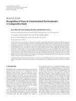
tasks such as object recognition or localization [5]. Figure 1
shows examples from a still camera and a DVD movie.
In previous work, a few methods have assumed no scene
motion, and use other cues such as lighting or varying zoom
[6]. However, the vast majority of current super-resolution
methods do assume motion, and either preregister the in-
puts using standard registration techniques, or assume that
a perfect registration is given a priori [1, 7], before carrying
out the super-resolution estimate. However, the steps taken
in super-resolution are seldom truly independent, and this
is too often ignored in current super-resolution techniques
[1, 7–12]. In this work we will develop two algorithms which
consider the problem in a more unified way.
The first approach is to estimate a super-resolution im-
age at the same time as finding the low-resolution image reg-
istrations. This simultaneous approach offers visible benefits
on results obtained from real data sequences. The registra-
tion model is fully projective, and we also incorporate a pho-
tometric model to handle brightness changes often present
in images captured in a temporal sequence. This makes
the model far more general than most super-resolution ap-
proaches. In contrast to fixed-registration methods—that is,
those like [7, 13], which first estimate and freeze the registra-
tion parameter values before calculating the super-resolution
image—we make use of the high-resolution image estimate
common to all the low-resolution images to improve the reg-

istration estimate.
An alternative approach, and the second one we explore,
is to marginalize over the unknown registration parameters.
This leads to a super-resolution algorithm which takes into
account the residual uncertainty in any image registration
estimate [14], taking the Bayesian approach of integrating
these unknown parameters out of the problem. We demon-
strate results on synthetic and real image data which shows
improved super-resolution results compared to the standard
fixed registration approach.
2 EURASIP Journal on Advances in Signal Processing
(a) Low-resolution image 1
(b) Low-resolution image 30
(c) Interpolated input 1
(d) Super resolved
(e) Low-res. image 1 (f) Low-res. image 20
(g) Interpolated input 1 (h) Super resolved
Figure 1: Examples of simultaneous MAP super-resolution. (a), (b) Two close-ups from a 30-frame digital camera sequence; (c) first image
interpolated into high-resolution frame; (d) simultaneous super-resolution output; (e), (f) two close-ups from a set of 29 DVD movie
frames; (g) first image interpolated into high-resolution frame (at corrected aspect ratio); (h) simultaneous super-resolution output.
The third component of this work introduces a scheme
by which the parameters of an image prior can be learnt in
the super-resolution framework even when there is possible
mis-registration in the input images. Poorly chosen prior val-
ues will lead to ill-conditioned systems or to overly-smooth
super-resolution estimates. Since the best values for any par-
ticular problem depend heavily on the statistics of the im-
age being super resolved and the characteristics of the input
dataset, having an online method to tune these parameters to
each problem is important.

The super-resolution model and notation are introduced
in Section 2, followed by the standard maximum a posteri-
ori (MAP) solution, and an overview of the ways in which it
is extended in this paper. The simultaneous registration and
super-resolution approach is developed in Section 3, and this
is followed by the learning of the prior parameters, which is
incorporated into the algorithm to give a complete simulta-
neous approach. Section 4 develops the marginalization ap-
proach by considering how to integrate over the registration
parameters.
Results on several challenging real datasets are used to il-
lustrate the efficacy of the joint MAP technique in Section 5,
as well as an illustration using synthetic data. Results using
the marginalization super-resolution algorithm are shown
for a subset of these datasets in Section 6. A discussion
of both approaches and concluding remarks are given in
Section 7.
1.1. Background
The work of Hardie et al. [5] has previously examined
the joint MAP image reg istration and super-resolution ap-
proach, but with a much more limited model. The high-
resolution estimate is used to update the image registrations,
but the motion model is limited to shifts on a quantized
grid (a 1/4-pixel spacing is used in their implementation),
so regist ration is a search across grid locations, which would
quickly become infeasible with more degrees of freedom.
Tipping and Bishop [15] marginalize out the hig h -
resolution image to learn a Euclidean registration directly,
but with such a high computational cost that their inputs
are restricted to 9

× 9pixels.Wesuggestitismorede-
sirable to integrate over the registration parameters rather
than the super-resolution image, because it is the registration
that constitutes the “nuisance parameters,” and the super-
resolution image that we wish to estimate.
With reference to learning the image prior, the gener-
alized cross validation (GCV) work of Nguyen et al. [12]
learns a regularization coefficient based on the data. All three
of the above approaches [5, 12, 15] rely on Gaussian image
priors, whereas a considerable body of super-resolution re-
search has demonstrated that there are many families of pri-
ors more suitable for image super-resolution [13, 16–20]. In
the following work, we use a more realistic image prior, not
a Gaussian.
Lyndsey C. Pickup et al. 3
Preliminary versions of the algorithms presented here ap-
pear in [21, 22].
2. THE ANATOMY OF MULTIFRAME
SUPER-RESOLUTION
A high-resolution scene x,withN pixels, is assumed to have
generated a set of K low-resolution images y
(k)
,eachwithM
pixels. For each image, the warping, blurring, and subsam-
pling of the scene is modelled by an M
×N sparse matrix W
(k)
[15, 18], and a global affine photometric correction results
from addition and multiplication across all pixels by scalars
λ

(k)
α
and λ
(k)
β
,respectively[18]. Thus the generative model is
y
(k)
= λ
(k)
α
W
(k)
x + λ
(k)
β
1 + 
(k)
,(1)
where

(k)
represents noise on the low-resolution image, and
consists of i.i.d. samples from a zero-mean Gaussian with
precision β (equivalent to std σ
N
= β
−1/2
), and images x and
y

(k)
are represented as vectors. The transform that maps be-
tween the frame of x and that of y
(k)
is assumed to be pa-
rameterized by some vector θ
(k)
(e.g., rotations, or an eight-
parameter projective transform), so W
(k)
is a function of θ
(k)
and of the image point-spread function (PSF), which ac-
counts for blur introduced by the camera optics and phys-
ical imaging process. Given
{y
(k)
}, the goal is to recover x,
without any explicit knowledge of
{θ
(k)
, λ
(k)
, σ
N
}.
For an individual low-resolution image y
(k)
,givenregis-
trations and x, the probability of having observed that image

is
p

y
(k)
| x, θ
(k)
, λ
(k)

=

β
2π

M/2
exp

−
β
2



y
(k)
− λ
(k)
α
W


θ
(k)

x − λ
(k)
β



2
2

,
(2)
which comes from (1), and from the assumption of Gaussian
noise. Other noise model choices lead to slightly different ex-
pressions, like the L
1
norm model of [19].
The vector x yielding the maximal value of p(y
(k)
|
x, θ
(k)
, λ
(k)
) would be the maximum likelihood (ML) solution
to the problem. However, the super-resolution problem is al-
most always poorly conditioned, so a prior over x is usually

required to avoid solutions which are subjectively very im-
plausible to the human viewer.
We choose a prior based on the Huber function, which
here will be applied to directional image gradients of the
super-resolution image. The Huber function takes a parame-
ter α, and for each directional image gradient z, it is defined:
ρ(z, α)
=

z
2
if |z| <α,
2α
|z|−α
2
otherwise.
(3)
The set of directional image gradients in the horizontal, ver-
tical, and two diagonal directions at all pixel locations in
x is denoted by G(x), and the prior probability of a high-
resolution image x is then
p(x)
=
1
Z
x
exp

−
ν

2

z∈G(x)
ρ(z, α)

,(4)
where ν is the prior strength parameter and Z
x
is a nor-
malization constant. The penalty for an individual direc-
tional gradient estimate z is quadra tic for small values of z,
which encourages smoothness, but the penalty is linear (i.e.,
less than quadratic) if z is large, which penalizes edges less
severely than a Gaussian.
In the next two sections, we will overview and contrast
the simultaneous max imum a posteriori and marginalization
approaches to the super-resolution problem. These two ap-
proaches will then be developed in Sections 3 and 4,respec-
tively.
2.1. Simultaneous maximum a posteriori
super-resolution
The maximum a posteriori (MAP) solution is found using
Bayes’ rule,
p

x |

y
(k)
, θ

(k)
, λ
(k)

=
p(x)

K
k
=1
p

y
(k)
| x, θ
(k)
, λ
(k)

p

y
(k)

|

θ
(k)
, λ
(k)


,
(5)
and by taking log s and neglecting terms which are not func-
tions of x or the registration parameters, this leads to the ob-
jective function
F
= β
K

k=1



y
(k)
− λ
(k)
α
W
(k)
x − λ
(k)
β
1



2
2

  
generative model
+ ν

z∈G(x)
ρ(z, α)
  
prior
.
(6)
In fixed-registration MAP super-resolution, W and λ values
are first estimated and frozen, typically using a feature-based
registration scheme (see, e.g., [7, 23]), then the intensities of
the registered images are corrected for photometric differ-
ences. The resulting problem is convex in x , and a gradient
descent algorithm, such as scaled conjugate gradients (SCG)
[24], will easily find the optimum at
∂F
∂x
= 0. (7)
In the simultaneous MAP approach here, we optimize F
explicitly with respect to x, the set of geometric registration
parameters θ (which parameterize W), and the photometric
parameters λ (composed of the λ
α
and λ
β
values), at the same
time, that is, we determine the point at which
∂F

∂x
=
∂F
∂θ
=
∂F
∂λ
= 0. (8)
The problem in (7)isconvex,becauseF is a quadratic
function of x. Unfortunately, the optimization in (8)isnot
necessarily convex with respect to θ. To see this, consider a
scene composed of a regularly tiled square texture: any two
θ values mapping two identical tiles onto each other will be
equally valid. However, we will show that a combination of
good initial conditions and weak priors over the variables of
interestallowsustoarriveatanaccuratesolution.
4 EURASIP Journal on Advances in Signal Processing
2.2. Marginalization super-resolution
In the approach above, which we term the joint MAP ap-
proach, we estimate x by maximizing over θ and λ.Nowina
second approach, the marginalization approach, we estimate
p(x
|{y
(k)
}) by marginalizing over θ and λ instead. In the
marginalization approach, a MAP estimate of x can then be
obtained by maximizing p(x
|{y
(k)
}) directly with respect to

x.
Using the identity
p(x
| d) =

p(x | d, t)p(t)dt,(9)
the integral over the unknown geometric and photometric
parameters,
{θ, λ},canbewrittenas
p

x |

y
(k)

=

p

x |

y
(k)
, θ
(k)
, λ
(k)

p


θ
(k)
, λ
(k)

d{θ, λ}
(10)
=

p(x)

K
k=1
p

y
(k)
| x, θ
(k)
, λ
(k)

p

y
(k)

|


θ
(k)
, λ
(k)

×
p

θ
(k)
, λ
(k)

d{θ, λ}
(11)
=
p(x)
p

y
(k)


K

k=1
p

θ
(k)

, λ
(k)

×
p

y
(k)
| x, θ
(k)
, λ
(k)

d{θ, λ},
(12)
where expression (11) comes from substituting (5) into (10),
and expression (12) uses the assumption that the images are
generated independently from the model [15] to take the de-
nominator out of the integral. Details of how this integral is
evaluated are deferred to Section 4, but notice that the left-
hand side depends only on x, not the registration parameters
θ and λ, and that on the right-hand side, the prior p(x)is
outside the integral.
3. SIMULTANEOUS SUPER-RESOLUTION WITH
MOTION AND PRIOR ESTIMATION
In this section, we fill out the details of the joint MAP image
registration and super-resolution approach, and couple it to
a scheme for learning the parameters of the image prior, to
form our complete simultaneous MAP super-resolution al-
gorithm.

The first key point is that in a ddition to optimiz-
ing the objective function (6) with respect to the super-
resolution image estimate x, we also optimize it w ith re-
spect to the geometric and photometric registration param-
eter set
{θ
(k)
, λ
(k)
}. This strategy closely resembles the well-
studied problem of bundle adjustment [25], in that the cam-
era parameters and image features are found simultane-
ously. Because most high-resolution pixels are observed in
most frames, the super-resolution problem is closest to the
“strongly convergent camera geometry” setup, and conjugate
gradient methods are expected to converge r apidly [25].
This optimization of the MAP objective function is inter-
leaved with a scheme to update the values of α and ν which
parameterize the edge-preserving image prior. This overall
super-resolution algorithm is assumed to have converged at
a point where all parameters change by less than a preset
threshold in successive iterations. An overview of the joint
MAP algorithm is given in Figure 1, and details of the learn-
ing of the prior are given in Section 3.3.
Section 3.1 offers a few comments on model suitability
and potential pitfalls. A sensible way of initializing the vari-
ous parts of the super-resolution problem helps it converge
rapidly to good solutions, so initialization details are given in
Section 3.2. Finally, Section 3.3 g ives details of the iterations
used to tune the values of the prior parameters.

3.1. Discussion of the joint MAP model
Errors in either geometric or photometric registration in the
low-resolution dataset have consequences for the estimation
of other super-resolution components. The u ncertainty in
localization can g ive the appearance of a larger point-spread
function kernel, because the effects of a scene point on the
low-resolution image set is more dispersed. Uncertainty in
photometric registration increases the variance of intensity
values at each spatial location, giving the appearance of more
low-resolution image noise, because low-resolution image
values will tend to lie further from the values of the back-
projected estimate. Increased noise in turn is an indicator
that a change in the prior weighting is required, thus light-
ing parameters can have a knock-on effect on the image edge
appearances.
By far the most difficultcomponentofmostsuper-
resolution systems to determine is the point-spread function
(PSF), which is of crucial importance, because it describes
how each pixel in x influences pixels in the observed images.
Resulting from optical blur in the camera, a rtifacts in the
sensor medium (film or a CCD array), and potentially also
through motion during the image exposure, the PSF is al-
most invariably modelled either as an isotropic Gaussian or a
uniform disk in super-resolution, though some authors sug-
gest other functions derived from assumptions on the cam-
era optics and sensor array [9, 16 , 26]. The exact shape of the
kernel depends on the entire process from photon to pixel.
Identifying and reversing the blur process is the domain
of blind image deconvolution. Approaches based on general-
ized cross-validation [27] or maximum likelihood [28]are

less sensitive to noise than other available techniques [29],
and both have direct analogs in current super-resolution
work [12, 15]. Because of the paramet ric nature of both
sets of algorithms, neither is truly capable of recovering
an arbitrary point-spread function. With this in mind, we
choose a few sensible forms of PSF and concentrate on super-
resolution which handles mismatches between the true and
assumed PSF as gracefully as possible.
3.2. Initialization and implementation details
There are convenient initializations for the geometric and
photometric registrations and for the high-resolution im-
age x, which by itself even gives a quick and reasonable
super-resolution estimate. Input images are assumed to be
Lyndsey C. Pickup et al. 5
(1) Initialize PSF, image regist rations, super-resolution image and prior parameters according to Section 3.2.
(2) (a) (Re)-sample the set of validation pixels (see Section 3.3).
(b) Update α and ν (prior parameters) using cross-validation-style gradient descent (see Section 3.3).
This includes a few steps of a suboptimization of F with respect to x.
(c) Optimize F (6) jointly with respect to x (super-resolution image), λ (photometric transform),
and θ (geometric transform). For SCG, the gradient expressions are given in (15) and (17).
(3) If the maximum absolute change in α, ν, or any element of x, λ,orθ is above preset convergence thresholds, return to (2).
Algorithm 1: Basic structure of the multiframe super-resolution algorithm with simultaneous image registration and learning of prior
parameter values.
preregistered by a standard algorithm such as RANSAC [23]
so that points at the image centres correspond to within a
small number of low-resolution pixels.
The image registration problem itself is not convex, and
repeating textures can cause naive intensity-based registra-
tion algorithms to fall into a local minimum, though when
initialized sensibly, very accurate results are obtained. The

pathological case where the footprints of the low-resolution
images fail to overlap in the high-resolution frame can be
avoided by adding an extra prior term to F to penalize large
deviations in the registration parameters from the initial reg-
istration estimate.
The initial registration estimate (both geometric and
photometric) is refined by optimizing the MAP objective
function F with respect to the registration parameters, but
using a cheap over-smooth approximation to x, known as
the average image, a [18]. Since a is a function of the regis-
tration parameters, it is recalculated at each step. Details of
the average image are given in Section 3.2.1, and the deriva-
tives expressions for the simultaneous optimization method
are given in (see Section 3.2.2).
Once
{θ
(k)
, λ
(k)
} have been estimated, the value of a can
be used as an initial estimate for x, and then the scaled con-
jugate g radients algorithm is applied to the ML cost function
(the first term of F ), but terminated after around K/4steps,
before the instabilities dominate because there is no prior.
This gives a sharper result than initializing with a as in [18 ].
When only a few images are available, a more stable ML so-
lution can be found by using a constrained optimization to
bound the pixel values so they must lie in the permitted im-
age intensity range.
In our system, the elements of x are scaled to lie in the

range [
−1/2, 1/2], and the geometric regist ration is decom-
pose into a “fixed” component, which is the initial mapping
from y
(k)
to x, and a projective correction term, which is it-
self decomposed into constituent shifts, rotations, axis scal-
ings, and projective parameters, which are the θ parameters,
then c oncatenated with λ to give one parameter vector. This
is then “whitened” to be zero mean and have a std of 0.35
units, which is approximately the standard deviation of x.
The prior over registration values suggested above is achie ved
simply by penalizing large values in this registration vector.
Boundary conditions are treated as in [15], making the
super-resolution image big enough so that the PSF kernel as-
sociated with any low-resolution pixel under any expected
registration is adequately supported. Gradients with respect
to x and λ can be found analytically, and those with respect
to θ are found numerical ly.
Finally, the prior parameters are initialized to around α
=
0.01 and ν = 0.1. We work with log α and log ν, since any real
value for these log quantities gives a positive value for ν and
α, which we require for the prior. For the PSF, a Gaussian
with std
≈ 0.45 low-resolution pixels is reasonable for in-
focus images, and a disk of radius upwards of 0.8 is suitable
for slightly defocused scenes.
3.2.1. The average image
The average image a is a stable though excessively smooth

approximation to x [18]. Each pixel in a is a weigh ted com-
bination of pixels in y such that a
i
depends strongly on y
j
if y
j
depends strongly on x
i
, according to the weights in W.
Lighting changes must also be taken into consideration, so
a
= S
−1
W
T
Λ
−1
α

y − Λ
β

, (13)
where W, y, Λ
α
,andΛ
β
are the stacks of the K groups of
W

(k)
, y
(k)
, λ
(k)
α
I,andλ
(k)
β
1,respectively,andS is a diagonal
matrix whose elements are the column sums of W.Notice
that both inverted matrices are diagonal, so a is simple to
compute. Using a in place of x, we optimize the first term of
F w ith respect to θ and λ only.Thisprovidesagoodestimate
for the registration parameters, without requiring x or the
prior parameters.
3.2.2. Gradient expressions for the simultaneous method
Defining the model fit error for the kth image as e
(k)
, so that
e
(k)
= y
(k)
− λ
(k)
α
W
(k)
x − λ

(k)
β
1, (14)
then the gradient of the objective function F (6)withrespect
to the super-resolution estimate x can be computed as
∂F
∂x
=−2β
K

k=1
λ
(k)
α
W
(k)T
e
(k)
− 2νD
T
ρ

(Dx, α), (15)
where Dx is a vector comprising all the elements of G(x), and
D itself is a large sparse mat rix. For each directional gradient
6 EURASIP Journal on Advances in Signal Processing
element z, the corresponding gradient element of the prior
term is given by
ρ


(z, α) =

2x,if|x|≤α,
2α sign (x), otherwise.
(16)
The gradients of the objective function with respect to
the registration parameters are given by
∂F
∂θ
(k)
i
=−2β

elements

λ
(k)
α
e
(k)
x
T

∂W
(k)
∂θ
(k)
i

,

∂F
∂λ
(k)
α
=−2βx
T
W
(k)
e
(k)
,
∂F
∂λ
(k)
β
=−2β
M

i
e
(k)
i
,
(17)
where
 is the Hadamard (element-wise) matrix product.
The W matrix represents the composition of spatial blur,
decimation, and resampling of the high-resolution image in
the frame of the low-resolution image, so even for a relatively
simple motion model (such as an affine homography with 6

degrees of freedom per image in the geometric registration
parameters), it is quicker to calculate the partial derivative
with respect to the parameters, ∂W
(k)
/∂θ
(k)
i
, using a central
difference approximation than to evaluate explicit derivatives
using the chain rule.
3.3. Learning the prior parameters with possible
registration error
It is necessary to determine ν and α of the Huber function of
(4) while still in the process of converging on the estimates of
x, θ,andλ. This is done by removing some individual low-
resolution pixels from the problem, solving for x using the
remaining pixels, then projecting this back into the original
image frames to determine its quality by the withheld vali-
dation pixels using a robust L
1
norm. The selected α and ν
should minimize this cross-validation error.
This defines a subtly different cross-validation approach
to those used previously for image super-resolution, because
validation pixels are selected at random from the collection
of K
× M individual linear equations comprising the over-
all problem, rather than from the K images. This distinc-
tion is important when uncertainty in the registrations is as-
sumed, since validation images can be misregistered in their

entirety. Assuming independence of the registration error on
each frame given x, the pixel-wise validation approach has a
clear advantage.
In determining a search direction in (ν, α)-space, F can
be optimized with respect to x, starting with the current x es-
timate, for just a few steps to determine whether the param-
eter combination improves the estimate. This intermediate
optimization does not need to run to convergence in order
to provide a gradient direction worthy of exploration. This
is much faster than the usual approach of running a com-
plete optimization for a number of parameter combinations,
especially useful if the initial estimate is poor. An arbitrary
5% of pixels are used for validation, ignoring regions within
a few pixels of edges, to avoid boundary complications, and
because inputs are centred on the region of interest.
4. THE MARGINALIZATION APPROACH
We now turn our attention to handling residual registration
uncertainty by considering distributions over possible reg-
istrations, then integrating these out of the problem. A set
of equations depending only upon the super-resolution es-
timate x, the input images
{y
(k)
}, and a starting estimate of
the registration parameter distributions are used to refine the
super-resolution estimate without having to maintain a reg-
istration estimate.
When the registration is known approximately, for in-
stance by preregistering inputs (as described in Section 3.2),
the uncertainty can be modeled as a Gaussian perturbation

about the mean estimate [
θ
(k)T
, λ
(k)
α
, λ
(k)
β
]
T
for each image’s
parameter set,
⎡
⎢
⎢
⎣
θ
(k)
λ
(k)
α
λ
(k)
β
⎤
⎥
⎥
⎦
=

⎡
⎢
⎢
⎢
⎣
θ
(k)
λ
(k)
α
λ
(k)
β
⎤
⎥
⎥
⎥
⎦
+ δ
(k)
, (18)
δ
(k)
∼ N (0, C),
(19)
p

θ
(k)
, λ

(k)

=



C
−1


(2π)
n

1/2
exp

−
1
2
δ
(k)T
C
−1
δ
(k)

.
(20)
In order to obtain an expression for p(x
|{y

(k)
})from
(2), (4), and (20), the parameter variations δ
(k)
must be in-
tegrated out of the problem, and details of this are given
in the following subsection. The diagonal matrix C is con-
structed to reflect the confidence in each parameter estimate.
This might mean a standard deviation of a tenth of a low-
resolution pixel on image translation parameters, or a few
grey levels’ shift on the illumination model, for instance.
4.1. Marginalizing over registration parameters
We now give details of how the integral is evaluated. With ref-
erence to (12), substituting in (2), (4), and (20), the integral
performed is
p

x |

y
(k)

=
1
p

y
(k)



β
2π

KM/2

b
2π

Kn/2
1
Z
x
× exp

−
ν
2

z∈G(x)
ρ(z, α)

×

exp

−
K

k=1


β
2
r
(k)
+
1
2
δ
(k)
C
(k)−1
δ
(k)


dδ,
(21)
Lyndsey C. Pickup et al. 7
where
r
(k)
=


e
(k)


2
2

,
δ
T
=

δ
(1)T
, δ
(2)T
, , δ
(K)T

,
(22)
and all the λ and θ parameters are functions of δ as in (18).
Expanding the data error term in the exponent for each
low-resolution image as a second-order Taylor series about
the estimated geometric registration parameter yields
r
(k)
(δ) ≈F
(k)
+ G
(k)T
δ +
1
2
δ
(k)T
H

(k)
δ
(k)
. (23)
Values for F, G,andH in our implementation are found nu-
merically (for geometric registrations) or analytically (for the
photometric parameters) from x and
{y
(k)
, θ
(k)
, λ
(k)
α
, λ
(k)
β
}.
Thus the whole exponent of (21), f ,becomes
f
=
K

k=1

−
β
2
F
(k)

−
β
2
G
(k)T
δ
(k)
−
1
2
δ
(k)T

β
2
H
(k)
+ C
−1

δ
(k)

=−
β
2
F
−
β
2

G
T
δ −
1
2
δ
T

β
2
H + V
−1

δ,
(24)
where the omission of image superscripts indicates stacked
matrices, and H is therefore a block-diagonal nK
×nK sparse
matrix, and V consists of the repeated diagonal of C.
Finally, letting S
= (β/2)H + V
−1
,

exp{ f }dδ =exp

−
β
2
F



exp

−
β
2
G
T
δ −
1
2
δ
T
Sδ

dδ
(25)
=exp

−
β
2
F

(2π)
nK/2
|S|
−1/2
exp


β
2
8
G
T
S
−1
G

.
(26)
The objective function, L to be minimized with respect
to x, is obtained by taking the negative log of (21), using the
result from (26), and neglecting the constant terms:
L
=
ν
2
ρ(Dx, α)+
β
2
F +
1
2
log
|S|−
β
2
8

G
T
S
−1
G. (27)
This can be optimized using SCG [24], noting that the gra-
dient can be expressed:
dL
dx
=
ν
2
D
T
d
dx
ρ(Dx)+
β
2
dF
dx
−
β
2
4
G
T
S
−1
dG

dx
+

β
4
vec

S
−1

T
+
β
3
16

G
T
S
−1
⊗ G
T
S
−1


d vec H
dx
,
(28)

where
⊗ is the Kronecker product and vec is the operation
thatvectorizesamatrix.DerivativesofF, G,andH with re-
spect to x can be found analytical ly for photometric parame-
ters, and numerically (using the analytic gr adient of e
(k)
(δ
(k)
)
with respect to x) with respect to the geometric parameters.
4.2. Discussion of the marginalization approach
It is possible to interpret the extra terms introduced into the
objective function in the derivation of the marginalization
method as an extra regularizer term or image prior. Consid-
ering (27), the first two terms are identical to the standard
MAP super-resolution problem using a Huber image prior.
The two additional terms constitute an additional distribu-
tion over x in the cases where S is not dominated by V; as the
distribution over θ and λ tightens to a single point, the terms
tend to constant values.
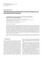
The intuition behind the method’s success (see Section 6 )
is that this prior will favor image solutions which are not
acutely sensitive to minor adjustments in the image registr a-
tion. The images of Figure 2 illustrate the type of solution
which would score poorly. To create the figure, one dataset
was used to produce two super-resolved images, using two
independent sets of registration parameters which were ran-
domly perturbed by an i.i.d. Gaussian vector with a standard
deviation of only 0.04 low-resolution pixels. The chequer-
board pattern typical of ML super-resolution images can be

observed, and the difference image on the r ight shows the
drastic contrast between the two image estimates.
4.3. Implementation details for parameter
marginalization
The terms of the Taylor expansion are found using a mixture
of analytic and numerical gradients. Notice that the value F
is simply the reprojection error of the current estimate of x
at the mean registration parameter values, and that gradients
of this expression with respect to the λ parameters, and with
respect to x can both be found analytically. To find the gra-
dient with respect to a geometric registration parameter θ
(k)
i
,
and elements of the Hessian involving it, a central difference
scheme involving only the kth image is used.
Mean values for the registration are computed by stan-
dard registration techniques, and x is initialized using
around 10 iterations of SCG to find the maximum likelihood
solution evaluated at these mean parameters. Additionally,
pixel values are scaled to lie between
−1/2and1/2, and the
ML solution is bounded to lie within these values in order
to curb the severe overfitting usually observed in ML super-
resolution results.
5. EXPERIMENTAL RESULTS FOR SIMULTANEOUS
MAP APPROACH
The performance of simultaneous registration, super-
resolution, and prior updating is evaluated using real data
from a variety of sources. Using the scaled conjugate gradi-

ents (SCG) implementation from Netlab [24], rapid conver-
gence is observed up to a point, beyond which a slow steady
decrease in F gives no subjective improvement in the solu-
tion, but this can be avoided by specifying sensible conver-
gence criteria.
The joint MAP results are contrasted with a fixed-
registration approach, where registrations between the in-
puts are found then fixed before the super-resolution process.
8 EURASIP Journal on Advances in Signal Processing
(a) Truth (b) ML image 1 (c) ML image 2 (d) Difference
Figure 2: An example of the effect of tiny changes in the registration parameters. (a) Ground truth image from which a 16-image low-
resolution dataset was generated. (b), (c) Two ML super-resolution estimates. In both cases, the same dataset was used, but the registration
parameters were perturbed by an i.i.d. vector with standard deviation of just 0.04 low-resolution pixels. (d) The difference between the two
solutions. In all these images, values outside the valid image intensity range have been rounded to white or black values.
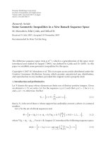
(a) Ground truth high resolution (b) Input 1/16 (c)Input2/16
Figure 3: Synthetic data: (a) ground tr uth image. (b), (c) Two example low-resolution images of 30 × 30 pixels, with clearly different
geometric and photometric registrations.
This fixed registration is found using the method described
in Section 3.2, a nd then (6) is optimized with respect only to
x to obtain a high-resolution estimate.
Synthetic dataset
Experiments are first performed on synthetic data, gener-
ated using the generative model (1) applied to a ground
truth image at a zoom factor of 4, with each pixel being cor-
rupted by additive Gaussian to give a SNR of 30 dB. Values
for a shift-only geometric registration, θ,anda2Dphoto-
metric registration λ are sampled independently from uni-
form distributions. The ground truth image and two of the
low-resolution images generated by the forward model are
shown in Figure 3. T he mean intensity is clearly different,

and the vertical shift is easily observed by comparing the top
and bottom edge pixels of each low-resolution image.
An initial registration was then carried out using an itera-
tive intensity-based scheme which optimized both geometric
and photometric parameters. This initial “fixed” registration
differs from the ground truth by an average of 0.0142 pixels,
and 1.00 grey levels for the photometric shift. Allowing the
joint MAP super-resolution algorithm to update this regis-
tration while super resolving the image resulted in registra-
tion errors of just 0.0024 pixels and 0.28 grey levels given the
optimal prior settings (see below and Figure 4).
We now sweep through values of the prior strength pa-
rameter ν, keeping the Huber parameter α set to 0.04. The
noise precision parameter β is chosen so that the noise is
assumed to have a standard deviation of 5 grey levels. For
each value of ν, both the fixed-registration and the joint MAP
methods are applied to the data, and the root mean square
error (RMSE) compared to the ground truth image is calcu-
lated.
The RMSE compared to the ground truth image for both
the fixed registration and the joint MAP approach are plot-
ted, in Figure 4, along with a curve representing the perfor-
mance if the ground truth registration is known. The prior
strength represented on the horizontal axis is log
10
(ν/β). Ex-
amples of the improvement in geometric and photometric
registration parameters are also shown.
Note that we have not learned the prior values in this
synthetic-data experiment, in order to plot how the value

of ν affects the output. We now evaluate the performance of
the whole simultaneous super-resolution algorithm, includ-
ing the learning of the ν and α values, on a selection of real
sequences.
Surrey library sequence
The camera motion is a slow pan through a smal l angle, and
the sign on a wall is illegible given any one of the inputs
alone. A s mall interest area of size 25
× 95 pixels is high-
lighted in the first of the 30 frames. Gaussian PSFs with std
=
0.375, 0.45, 0.525 are selected, and used in both algorithms.
There are 77003 elements in y,andx has 45936 elements
with a zoom factor of 4. W has around 3.5
× 10
9
elements, of
which around 0.26% are nonzero with the smallest of these
Lyndsey C. Pickup et al. 9
10
15
20
25
30
RMSE (grey levels)
−4 −3 −2 −1
Prior strength
RMSE with respect to g round
truth image
Fixed registration

Joint MAP registration
Ground truth registration
(a)
−0.4
−0.2
0
0.2
0.4
0.6
Vertical shift
−0.50 0.5
Horizontal shift
Geometric parameters
(b)
−10
−5
0
5
10
λ
β
(additive term)
0.811.21.4
λ
α
(multiplicative factor)
Photometric parameters
(c)
Figure 4: Synthetic data plots. (a) RMSE compared to ground truth, plotted for the fixed and joint MAP algorithms, and for the Huber
super-resolution image found using the ground truth registration. (b), (c) plots showing the registration values for the initial (orange “+”),

joint MAP (blue “
×”) and ground truth ( black “◦”) registrations. In most cases, the joint MAP registration value is considerably closer to
the true value than the initial “fixed” value is.
(a) Image 1 (whole)
(b) Fixed reg. σ = 0.375
(c) Fixed reg. σ = 0.45
(d) Fixed reg. σ = 0.525
(e) Simul. reg. σ = 0.375
(f) Simul. reg. σ = 0.45
(g) Simul. reg. σ = 0.525
Figure 5: Surrey library sequence. (a) One of the 30 original images. (b), (c), (d) Super-resolution found using fixed registrations. (e), (f),
(g) Super-resolution images using simultaneous MAP algorithm. Detailed regions of two of the low-resolution images can be seen in Figures
1(a), 1(b).
PSF kernels, and 0.49% with the largest. Most instances of the
simultaneous a lgorithm converge in 2 to 5 iterations. Results
are shown in Figure 5, showing that while both algorithms
perform well with the middle PSF size, the simultaneous-
registration algorithm handles deviations from this optimum
more gracefully.
“
ˇ
Ceskoslovensko” sequence
The ten images in this sequence were captured on a rig
which constrained the motion to be pure translation, though
photometric differences are very apparent in the input im-
ages. Gaussian PSFs with std
= 0.325, 0.40, 0.475 are used in
both super-resolution algorithms. The results are shown in
Figure 6, and the lines and text are much more clearly de-
fined in the super-resolution version.

Eye-test card sequence
The second real-data experiment uses just 10 images of an
eye-test card, captured using a webcam. The card is tilted
and rotated slightly, and image brightness varies as the light-
ing and camera angles change. Gaussian PSFs with std
=
0.30, 0.375, 0.45 are used in both super-resolution algo-
rithms. The results are shown in the left portion of Figure 7.
Note that the last row is illegible in the low-resolution im-
ages, but can be read in the super-resolution images.
Camera “9” sequence
The model is adapted to handle DVD input, where the aspect
ratio of the input images is 1.25 : 1, but they represent 1.85 : 1
video. The correction in the horizontal scaling is incorpo-
rated into the “fixed” part of the homography representation,
and the PSF is assumed to be radially symmetric. This avoids
10 EURASIP Journal on Advances in Signal Processing
(a) Image 1
(b) Image 1, detail
(c) Image 10, detail
(d) Fixed reg, σ = 0.4
(e) Simul reg, σ = 0.4
Figure 6: “
ˇ
Ceskoslovensko” sequence. (a) The first image in the sequence. (b), (c) details of the region of interest in the first and last low-
resolution images. (d) Super-resolution found using fixed registrations. (e) Super-resolution images using simultaneous MAP algorithm.
an undesirable interpolation of the inputs prior to super re-
solving, which would lose high-frequency information, and
also avoids working with squashed super-resolution images
throughout the process, which would violate the assumption

of an isotropic prior over x. In short, we do not scale any
of the images, but instead work with inputs and outputs at
different aspect rat ios.
The Camera “9” sequence consists of 29 I-frames
1
from
the movie Groundhog Day. An on-screen hand-held TV cam-
era moves independently of the real camera, and the logo on
the side is chosen as the interest region. Disk-shaped PSFs
with radii of 1.0, 1.4, and 1.8 pixels are used. In b oth the
eye-test card and Camera “9” sequences, the simultaneously
optimized super-resolution images again appear subjectively
better to the human viewer, and are more consistent across
different PSFs.
Lola Rennt sequences
Finally, results obtained from difficult DVD input sequences
that were taken from the movie Lola Rennt are shown in
Figure 8. In the “cars” sequence, there are just 9 I-frames
showing a pair of cars, and the areas of interest are the car
number plates. The “badge” sequence shows the badge of a
bank security officer. Seven I-frames are available, but are all
dark, making the noise level proportionally very high. Signif-
icant improvements at a zoom factor of 4 (in each direction)
can be seen.
6. EXPERIMENTAL RESULTS FOR THE
MARGINALIZATION APPROACH
The performance of the marginalization approach was evalu-
ated in a similar way to the simultaneous joint MAP method
of Section 5. The objective function (27) was optimized di-
rectly with respect to the super-resolution image pixels, first

1
I-frames are encoded as complete images, rather than requiring nearby
frames in order to render them.
working on synthetic datasets with known ground truth, and
then on real-data sequences. Results are compared with the
fixed-registration Huber-MAP method, and with the simul-
taneous joint MAP method.
Synthetic experiments
The first experiment takes a sixteen-image synthetic dataset
created from the eyechart image of Figure 3(a). The dataset
is generated using the same procedure as already described,
except that the subpixel perturbations are evenly spaced over
a grid up to plus or minus one half of a low-resolution pixel,
giving a similar setup to that described in [12],butwithad-
ditional lighting variation.
The images giving lowest RMS error from each set are
displayed in Figure 9. The lowest RMSE for the marginal-
izing approach is 11.73 grey levels, and the corresponding
RMSE for the registration-fixing approach is 14.01. Using
the L
1
norm (mean absolute pixel difference), the error is
3.81 grey levels for the fixed-registration approach, and 3.29
for the marginalizing approach proposed here. The standard
deviation of the prior over θ is set to 0.004, which is found
empirically to give good results. Visually, the differences be-
tween the images are subtle, though the bottom row of letters
is better defined in the marginalization approach.
The RMSE for three approaches (fixed registration, joint
MAP, and marginalizing) is plotted in Figure 10, and again

the horizontal axis represents log
10
(ν/β). The dotted orange
curve reflects the error from the fixed-registration approach
using the registration estimated from the low-resolution in-
puts. Both the joint MAP (blue curve) and marginalization
(green curve) approaches obtain lower errors, closer to those
obtained if the ground truth registration is known (dashed
black curve).
Note that while the lowest error values are achieved using
the joint MAP approach, the results using the marginaliza-
tion approach are obtained using only the initial (incorrect)
registration values. The marginalization approach also stays
consistently good over a wider range of possible prior values,
making it more robust than either of the other methods to
Lyndsey C. Pickup et al. 11
(a) Selection from
first eyechart frame
(b) Selection from
eighteyechartframe
(c) Original DVD frame (camera
9sequence)
Fixed σ = 0.3Sim.σ = 0.3Fixedr = 1Sim.r = 1
Fixed σ = 0.375 Sim. σ = 0.375 Fixed r = 1.4Sim.r = 1.4
Fixed σ = 0.45 Sim. σ = 0.45 Fixed r = 1.8Sim.r = 1.8
Figure 7: Eyechart sequence and camera “9” sequence. (a), (b) Sections of two input images from the 10-frame eye-test card sequence.
Notice the card appears much brighter in the left image. (c) Raw DVD frame for camera “9” sequence (see Figure 1 for close-up of interest
region). Lower section, first and third columns: results obtained by fixing registration prior to super resolution. Lower section, second and
fourth columns: results obtained using the simultaneous approach to optimize the super-resolution image, registration parameters, and
prior parameters.

poor estimates of the prior distribution, or of the precision β
of the noise on the input dataset.
Real data
We again use the “
ˇ
Ceskoslovensko,” which is seen in Figure 6.
Image registration was carried out in the same manner as be-
fore, and the geometric parameters agree with the provided
homographies to within a few hundreds of a pixel. Super-
resolution images were created for a number of ν values, and
subjectively, the equivalent values to those quoted in [18]
were selected for the Huber recovery. As with the synthetic
data, a slightly larger ν value was chosen for the registration-
marginalizing output, and a similar covariance of the reg-
istration parameters was assumed. We also compare against
Tipping and Bishop’s method [15],whichwehaveextended
to cover the illumination model and used to register and su-
per resolve the dataset, using the same PSF value (0.4low-
resolution pixels) as the other methods.
The three sets of results on the real-data sequence are
shown in the middle and bottom rows of Figure 11.Tofacil-
itate a better comparison, a subregion of each is expanded to
make the letter details clearer. The Huber prior used alone in
the fixed-registr ation method tends to make the edges unnat-
urally sharp, though it is very successful at regularizing the
solution elsewhere. The text in the marginalizing approach’s
image appears clearer than the text in the image found using
Tipping and Bishop’s method, and the regularization in the
constant background regions is slightly more successful.
7. CONCLUSIONS

This work has examined two methods of considering the im-
age registration and other parts of the super-resolution prob-
lem at the same time as the high-resolution image estimate,
and illustrated these with examples where both methods give
improvements in the quality of the resulting super-resolved
image.
Firstly, we showed that optimizing the MAP image so-
lution with respect to the low-resolution image registration
parameters as well as the high-resolution pixel values yields
a better solution than the two-phase register-then-super-
12 EURASIP Journal on Advances in Signal Processing
Original DVD frame (cars sequence) Original DVD frame (badge sequence)
(a)
(b)
Sim. × 4, σ = 0.55 Sim. × 4, σ = 0.55 Sim. × 4, r = 1.2
(c)
Figure 8: Results from the simultaneous super-resolution, image registration, and prior parameter updating scheme applied to the movie
Lola Rennt on DVD. (a): two raw DVD frames. (b): five low-res frames from each sequence (black car’s number plate, white car’s number
plate, security guard’s ID badge). (c): the same image regions super resolved using the simultaneous method. In the case of the security
guard’s ID badge, intensities have been scaled for ease of viewing. Please refer to the text for notes on the aspect ratios involved when
working with DVD frames.
resolve approach conventionally used. In addition to this, our
MAP algorithm included a cross-validation step to select a
prior distribution appropriate for the scene statistics, which
could be incorporated without great additional expense into
the iterative recovery algorithm.
Secondly, we developed an alternative approach using
Bayesian marginalization within the super-resolution model,
with several advantages over Tipping and Bishop’s original
algorithm. These are: a formal t reatment of registration un-

certainty, the use of a much more realistic image prior, and
the computational speed and memory efficiency relating to
the smaller dimension of the space over which we integrate.
The results on real and synthetic images with this method
show an advantage over the fixed-registration approach, and
over the result from Tipping and Bishop’s method, largely
owing to our more favourable prior over the super-resolution
image.
In future work, a combination of these methods may
prove most accurate, with the registration improvement of
the simultaneous method providing a stronger starting point
for the marginalization approach, as well as a very accu-
rate initial sup er-resolution image estimate. It seems plau-
sible that image accuracy could be improved considerably by
swapping the Huber prior used here with another more spe-
cialized or domain-specific image prior [20, 30].
ACKNOWLEDGMENTS
The “library” data sequence used in Figures 1 and 5 is
due to Barbara Levienaise-O badia, University of Surrey,
Lyndsey C. Pickup et al. 13
Best fixed (err. = 14.01)
(a)
Best int. (err. = 11.73)
(b)
Figure 9: Synthetic dataset results. (a) The best (minimum MSE)
image from the fixed-registration algorithm, having super resolved
the dataset multiple times with different prior strength settings. (b)
The best result using our approach of integrating over θ and λ.As
well as having a lower RMSE, note the improvement in black-white
edge detail on some of the letters on the bottom line.

10
15
20
25
RMSE (grey levels)
−4.5 −4 −3.5 −3 −2.5 −2 −1.5 −1
Prior strength
RMSE with respect to ground truth image
Fixed registration
Joint MAP registration
Marginalizing approach
Ground truth registration
Figure 10: Plot showing the variation of RMSE with prior strength
for the fixed Huber MAP method and our approach integrating over
θ and λ, applied to the synthetic dataset of Figure 9.Aswellasreach-
ing a lower minimum, the integrating approach appears to be more
consistent across variations in pr ior strength.
(a) Integrating θ, λ (b) Integrating θ, λ (de-
tailed region)
(c) Fixed MAP (detailed
region)
(d) Tipping and Bishop
(detailed region)
Figure 11: (a) The full super-resolution output from our algorithm.
(b) Detailed region of the central letters, again with our algorithm.
(c) Detailed region of the regular Huber MAP super-resolution im-
age, using parameter values suggested in [18], which are also found
to be subjectively good choices. The edges are slightly artificially
crisp, but the large smooth regions are well regularized. (d) Close-
up of letter detail for comparison with Tipping and Bishop’s method

of marginalization. The Gaussian form of their prior leads to a more
blurred output, or one that over fits to the image noise present on
the input data.
and the constrained-motion dataset of Figure 11 is due
to Tomas Pajdla and Daniel Martinec, CMP, Prague.
Both datasets are available for download from http://www
.robots.ox.ac.uk/
∼vgg/data. This work was funded in part by
EC Network of Excellence PASCAL and by the EPSRC. David
Capel is with 2D3, .
REFERENCES
[1] M. Irani and S. Peleg, “Super resolution from image se-
quences,” in Proceedings of the 10th Internat ional Conference
on Pattern Recognition (ICPR ’90), vol. 2, pp. 115–120, Atlantic
City, NJ, USA, June 1990.
[2]A.J.Patti,M.I.Sezan,andA.M.Tekalp,“Robustmethods
for high-quality s tills f rom interlaced video in the presence of
dominant motion,” IEEE Transactions on Circuits and Systems
for Video Technology, vol. 7, no. 2, pp. 328–342, 1997.
[3] Salient Stills, />[4] P. Cheeseman, B. Kanefsky, R. Kraft, J. Stutz, and R. Han-
son, “Super-resolved surface reconstruction from multiple
images,” in Maximum Entropy and Bayesian Methods,G.R.
Heidbreder, Ed., pp. 293–308, Kluwer Academic Publishers,
Dordrecht, The Netherlands, 1996.
[5] R. C. Hardie, K. J. Bar nard, and E. E. Armstrong, “Joint MAP
registration and high-resolution image estimation using a se-
quence of undersampled images,” IEEE Transactions on Image
Processing, vol. 6, no. 12, pp. 1621–1633, 1997.
[6] M. V. Joshi, S. Chaudhuri, and R. Panuganti, “A learning-
based method for image super-resolution from zoomed obser-

vations,” IEEE Transactions on Systems, Man, and Cybernetics,
Part B, vol. 35, no. 3, pp. 527–537, 2005.
[7] D. P. Capel and A. Zisserman, “Automated mosaicing with
super-resolution zoom,” in Proceedings of the IEEE Computer
SocietyConferenceonComputerVisionandPatternRecogni-
tion (CVPR ’98), pp. 885–891, Santa Barbara, Calif, USA, June
1998.
[8] Y. Altunbasak, A. J. Patti, and R. M. Mersereau, “Super-
resolution still and video reconstruction from MPEG-coded
video,” IEEE Transactions on Circuits and Systems for Video
Technology, vol. 12, no. 4, pp. 217–226, 2002.
[9] S. Baker and T. Kanade, “Limits on super-resolution and how
to break them,” IEEE Transactions on Pattern Analysis and Ma-
chine Intelligence, vol. 24, no. 9, pp. 1167–1183, 2002.
[10] B. Bascle, A. Blake, and A. Zisserman, “Motion deblurring and
super-resolution from an image sequence,” in Proceedings of
the 4th European Conference on Computer Vision (ECCV ’96),
vol. 2, pp. 573–582, Springer, Cambridge, UK, April 1996.
[11] M. Elad and A. Feuer, “Restoration of a single superresolution
image from several blurred, noisy, and undersampled mea-
sured images,” IEEE Transactions on Image Processing, vol. 6,
no. 12, pp. 1646–1658, 1997.
[12] N. Nguyen, P. Milanfar, and G. Golub, “Efficient general-
ized cross-validation with applications to parametric image
restoration and resolution enhancement,” IEEE Transactions
on Image Processing, vol. 10, no. 9, pp. 1299–1308, 2001.
[13] R. R. Schultz and R. L. Stevenson, “A Bayesian approach to
image expansion for improved definition,” IEEE Transactions
on Image Processing, vol. 3, no. 3, pp. 233–242, 1994.
[14] D. Robinson and P. Milanfar, “Fundamental performance lim-

its in image registration,” IEEE Transactions on Image Process-
ing, vol. 13, no. 9, pp. 1185–1199, 2004.
14 EURASIP Journal on Advances in Signal Processing
[15] M. E. Tipping and C. M. Bishop, “Bayesian image super-
resolution,” in Proceedings of Advances in Neural Information
Processing Systems 15 (NIPS ’02), pp. 1279–1286, Vancouver,
British Columbia, Canada, December 2002.
[16] S. Borman, Topics in multiframe superresolution restoration,
Ph.D. thesis, University of Notre Dame, Notre Dame, Ind,
USA, May 2004.
[17] S. Borman and R. L. Stevenson, “Simultaneous multi-frame
MAP super-resolution video enhancement using spatio-
temporal priors,” in Proceedings of International Conference on
Image Processing (ICIP ’99), vol. 3, pp. 469–473, Kobe, Japan,
October 1999.
[18] D. P. Capel, Image Mosaicing and Super-Resolution, Distin-
guished Dissertations, Springer, New York, NY, USA, 2004.
[19] S. Farsiu, M. Elad, and P. Milanfar, “A practical approach to
super-resolution,” in Visual Communications and Image Pro-
cessing, vol. 6077 of Proceedings of SPIE,SanJose,Calif,USA,
January 2006.
[20] L. C. Pickup, S. J. Roberts, and A. Zisserman, “A sampled tex-
ture prior for image super-resolution,” in Proceedings of Ad-
vances in Neural Information Processing Systems 16 (NIPS ’03),
pp. 1587–1594, Vancouver, British Columbia, Canada, De-
cember 2004.
[21] L. C. Pickup, D. P. Capel, S. J. Roberts, and A. Zisserman,
“Bayesian image super-resolution, continued,” in Advances
in Neural Information Processing Systems 19, pp. 1089–1096,
Cambridge, Mass, USA, December 2006.

[22] L. C. Pickup, S. J. Roberts, and A. Zisserm an, “Optimizing
and learning for super-resolution,” in Proceedings of the 17th
British Machine Vision Conference (BMVC ’06), Edinburgh,
UK, September 2006.
[23] R. I. Hartley and A. Zisserman, Multiple View Geometry in
Computer V ision, Cambridge University Press, Cambridge,
UK, 2nd edition, 2004.
[24] I. Nabney, NETLAB: Algorithms for Pattern Recognition,
Springer, New York, NY, USA, 2002.
[25] B. Triggs, P. F. McLauchlan, R. I. Hartley, and A. W. Fitzgib-
bon, “Bundle adjustment—a modern synthesis,” in Proceed-
ings of International Workshop on Vision Algorithms on Vision
Algorithms: Theory and Practice, B. Triggs, A. Zisser m an, and
R. Szeliski, Eds., vol. 1883 of Lecture Notes in Computer Science,
pp. 298–372, Springer, Corfu, Greece, September 1999.
[26] R.C.Hardie,K.J.Barnard,J.G.Bognar,E.E.Armstrong,and
E. A. Watson, “High-resolution image reconstruction from a
sequence of rotated and translated frames and its application
to an infrared imaging system,” Optical Engineering, vol. 37,
no. 1, pp. 247–260, 1998.
[27] S. J. Reeves and R. M. Mersereau, “Blur identification by the
method of generalized cross-validation,” IEEE Transactions on
Image Processing, vol. 1, no. 3, pp. 301–311, 1992.
[28] R. L. Lagendijk, A. M. Tekalp, and J. Biemond, “Maximum
likelihood image and blur identification: a unifying approach,”
Optical Engineering, vol. 29, no. 5, pp. 422–435, 1990.
[29] D. Kundur and D. Hatzinakos, “Blind image deconvolution,”
IEEE Signal Processing Magazine, vol. 13, no. 3, pp. 43–64,
1996.
[30] W. T. Freeman, T. R. Jones, and E. C. Pasztor, “Example-based

super-resolution,” IEEE Computer Graphics and Applications,
vol. 22, no. 2, pp. 56–65, 2002.
Lyndsey C. Pickup is a Researcher in the
Machine Learning Group and Visual Ge-
ometry Groups at the University of Ox-
ford. She graduated from Keble College,
University of Oxford, with first class hon-
ours in engineering and computing science
in 2002. Her interests lie in the application
of Bayesian methods to computer vision,
and specifically in handling noise and un-
certainty in super-resolution without over-
simplifying the image model.
David P. Capel received the M.Eng. degree
in engineering and computing science from
Oxford University in 1996. He completed
his Ph.D. degree on image mosaicing and
super-resolution as part of the Visual Ge-
ometry Group, also at Oxford University, in
2001. Since then, he has worked as a Vision
Scientist at 2d3 Ltd., contributing to the
development of the Emmy award-winning
camera tracking software, “boujou.” In his
current role as Lead Scientist for 2d3’s Advanced Imagery Group,
he focuses on computer vision applications for aerial imagery. His
research interests are in real-time computer vision and video en-
hancement, sensor fusion for long-range camera tracking, and au-
tomatic scene reconstruction.
Stephen J. Roberts’ main area of research
lies in machine learning approaches to data

analysis. He has particular interests in the
development of machine learning theory
for problems in time series analysis and de-
cision theory. His current research applies
Bayesian statistics, graphical models, and
information theory to diverse problem do-
mains including mathemetical biology, fi-
nance, and sensor fusion. He runs the Pat-
tern Analysis and Machine Learning Research Group at the Univer-
sity of Oxford and is a fellow of Somerville College, Oxford.
Andrew Zisserman is the RAE/Microsoft Professor of computer
vision at the Department of Engineering Science, University of
Oxford, where he heads the Visual Geometry Group. He gradu-
ated from the University of Cambridge with a degree in theoretical
physics, and for the last 20 years has carried out research in com-
puter vision. He has coauthored and coedited several books on this
area. The most recent, Multiple View Geometry in Computer Vision
(written with Richard Hartley), has now been published as a sec-
ond edition in paperback and also translated into Chinese. He has
been a Program Chair and a General Chair for the IEEE Interna-
tional Conference on Computer Vision. He was elected a fellow of
the Royal Society in 2007.