Báo cáo hóa học: " Research Article Nonconcave Utility Maximisation in the MIMO Broadcast Channel" pdf

Hindawi Publishing Corporation
EURASIP Journal on Advances in Signal Processing
Volume 2009, Article ID 645041, 13 pages
doi:10.1155/2009/645041
Research Article
Nonconcave Utility Maximisation in
the MIMO Broadcast Channel
Johannes Brehmer and Wolfgang Utschick
Associate Institute for Signal Processing, Technische Universit
¨
at M
¨
unchen, 80333 Munich, Germany
Correspondence should be addressed to Johannes Brehmer,
Received 15 February 2008; Accepted 12 June 2008
Recommended by S. Toumpis
The problem of determining an optimal parameter setup at the physical layer in a multiuser, multiantenna downlink is considered.
An aggregate utility, which is assumed to depend on the users’ rates, is used as performance metric. It is not assumed that the
utility function is concave, allowing for more realistic utility models of applications with limited scalability. Due to the structure of
the underlying capacity region, a two step approach is necessary. First, an optimal rate vector is determined. Second, the optimal
parameter setup is derived from the optimal rate vector. Two methods for computing an optimal rate vector are proposed. First,
based on the differential manifold structure offered by the boundary of the MIMO BC capacity region, a gradient projection
method on the boundary is developed. Being a local algorithm, the method converges to a rate vector which is not guaranteed
to be a globally optimal solution. Second, the monotonic structure of the rate space problem is exploited to compute a globally
optimal rate vector with an outer approximation algorithm. While the second method yields the global optimum, the first method
is shown to provide an attractive tradeoff between utility performance and computational complexity.
Copyright © 2009 J. Brehmer and W. Utschick. This is an open access article distributed under the Creative Commons Attribution
License, which permits unrestricted use, distribution, and reproduction in any medium, provided the original work is properly
cited.
1. Introduction
The majority of current wireless communication systems are

based on the principle of orthogonal multiple access. Simply
speaking, multiple users compete for a set of shared channels,
and access to the channels is coordinated such that each
channel is used by a single user only. The decision which
user accesses which channel is made at the medium access
(MAC) layer, with the result that at the physical (PHY) layer,
transmission is over single-user channels. Based on recent
advances in physical layer techniques such as MIMO signal
processing and multiuser coding, it has been shown that
significant performance gains can be achieved by allowing
one channel to be used by multiple users at once [1–5]. In
other words, the physical layer paradigm is shifting from
single-user channels to multiuser channels. This change also
dissolves the strict distinction between MAC and PHY layers,
as the question which users access which channels can only
be answered in a joint treatment of both layers.
In this work, a multiuser, multiantenna downlink in a
single-cell wireless system is considered, which, from the
viewpoint of information theory, corresponds to a MIMO
broadcast channel (MIMO BC) [3, 6]. While the aforemen-
tioned shift to multiuser channels is motivated by the poten-
tial gains in system performance, an evident drawback of
this shift is the increased design complexity. In other words,
multiantenna, multiuser channels significantly increase the
set of design parameters and degrees of freedom at the PHY
layer. Clearly, strategies for tuning these parameters in an
optimal manner are of great interest.
The desire for maximum system performance leads
immediately to the question of optimality criteria. While
voice and best effort data applications have been predom-

inant, future wireless systems are expected to provide a
multitude of heterogeneous applications, ranging from best
effort data to low-delay gaming applications, from low-rate
messaging to high-rate video. The heterogeneity of these
applications requires application-aware optimality criteria,
that is, it is no longer sufficient to optimise PHY and MAC
layers with respect to criteria such as average throughput
or proportional rate fairness. Utility functions have been
widely used as a model for the properties of upper layers.
2 EURASIP Journal on Advances in Signal Processing
In this work, the focus is on the optimisation of the PHY
layer parameters, and a generic utility model in terms of a
function that is monotone in the users’ rates is employed.
For a wide range of applications, utility models can be found
in the literature. In [7], applications are classified based
on their elasticity with respect to the allocated rate. Best
effort applications can be modelled with a concave utility
[7]. On the other hand, less elastic applications result in a
nonconcave utility model [7, 8]. While most works on utility
maximisation in wireless systems assume concave utilities,
the nonconcave setup has received relatively little attention
[8–10]. Based on the premise that some relevant application
classes can be more precisely modelled by nonconcave
utilities, this work proposes a solution strategy that provides
at least locally optimal performance in the nonconcave case.
There exists a significant amount of literature on utility
maximisation for wireless networks, see, for example, [10–
13] and references therein. The network-oriented works
usually consider a large number of nodes with a simple
physical layer setup, and focus on computationally efficient

and distributed resource allocation strategies for large net-
works. In contrast, this work focuses on the optimisation
of a limited-size infrastructure network with a complex
multiantenna, multiuser PHY/MAC layer configuration.
Utility maximisation in the MIMO BC is also investi-
gated in [14]. The authors solve the utility maximisation
problem based on Lagrange duality, under the assumption
of concave utility functions. Dual methods are frequently
used in network utility maximisation [10], but rely on
the assumption of problem convexity. This work makes
the following contributions. First, a primal gradient-based
method for addressing the utility maximisation problem in
the MIMO BC is developed. The proposed method does not
rely on a convexity assumption and can provide convergence
to local optima in the nonconvex case. The quality of such
local solutions depends on the specific problem instance
and can only be evaluated if the global optimum is known.
The second contribution of this work is the application of
methods from the field of deterministic global optimisation
to the nonconcave utility maximisation problem. It is shown
that the utility maximisation problem in the MIMO BC
can be cast as a monotonic optimisation problem [15].
The monotonicity structure can be exploited to efficiently
find the global optimum by an outer approximation algo-
rithm.
Notation. Vectors and vector-valued functions are denoted
by bold lowercase letters, matrices by bold uppercase letters.
The transpose and the Hermitian transpose of Q are denoted
by Q
T

and Q
H
, respectively. The identity matrix is denoted by
1. Concerning boldface, an exception is made for gradients.
The gradient of a function u evaluated at x is a vector
∇u(x), the gradient of a function f evaluated at x is a matrix
∇f(x) whose ith column is the gradient at x of the ith
component function of f [16]. The following definitions of
order relations between vectors x, y
∈ R
K
,withK>1, are
used:
x
≥ y ⇐⇒ ∀ k : x
k
≥ y
k
,
x > y
⇐⇒ x ≥ y, ∃k : x
k
>y
k
,
x
 y ⇐⇒ ∀ k : x
k
>y
k

.
(1)
Order relations
≤, <,  are defined in the same manner.
2. Problem Setup
At the physical layer, a MIMO broadcast channel with K
receivers is considered. The transmitter has N transmit
antennas, while receiver k is equipped with M
k
receiving
antennas. The transmitter sends independent information to
each of the receivers.
The received signal at receiver k is given by
y
k
= H
k
K

i=1
x
i
+ η
k
,(2)
where H
k
∈ C
M
k

×N
is the channel to receiver k and x
k
∈ C
N
is the signal transmitted to receiver k. Furthermore, η
k
is the
circularly symmetric complex Gaussian noise at receiver k,
with η
k
∼CN (0, 1
M
k
).
Let Q
k
denote the transmit covariance matrix of user k.
The total transmit power has to satisfy the power constraint
tr(

K
k
=1
Q
k
) ≤ P
tr
. Accordingly, with Q = (Q
1

, , Q
K
) the
set of feasible transmit covariance matrices is given by
Q
=

Q : Q
k
∈ H
N
+
,tr

K

k=1
Q
k

≤
P
tr

,(3)
where H
N
+
denotes the set of positive semidefinite Hermitian
N

×N matrices.
As proved in [6], capacity is achieved by dirty paper
coding (DPC). Let π denote the encoding order, that is, π :
{1, , K}→{1, , K}is a permutation, and π(i) is the index
of the user which is encoded at the ith position. Moreover, let
Π denote the set of all possible permutations on
{1, , K}.
For fixed Q and π,anachievableratevectorisgivenby
r(Q, π)
= (r
1
(Q, π), , r
K
(Q, π)), with
r
π(i)
= log
det

1 + H
π(i)


j≥i
Q
π( j)

H
H
π(i)


det

1 + H
π(i)


j>i
Q
π( j)

H
H
π(i)

. (4)
Let R denote the set of rate vectors achievable by feasible Q
and π:
R
=

r(Q, π):Q ∈ Q, π ∈ Π

. (5)
The capacity region of the MIMO BC is defined as the convex
hull of R [3]:
C
= co(R). (6)
Accordingly, each element of C can be written as a convex
combination of elements of R, that is, for each r

∈ C, there
exists a set of coefficients
{α
w
}, a set of transmit covariance
matrices
{Q
(w)
}, and a set of encoding orders {π
(w)
} such
that
r
=
W

w=1
α
w
r

Q
(w)
, π
(w)

,(7)
EURASIP Journal on Advances in Signal Processing 3
with α
w

≥ 0,

W
w
=1
α
w
= 1, Q
(w)
∈ Q,andπ
(w)
∈ Π. In other
words, r is achieved by time-sharing between rate vectors
r(Q
(w)
, π
(w)
) ∈ R.
Each r
∈ C can be achieved by time-sharing between
at most K rate vectors r(Q
(w)
, π
(w)
) ∈ R,thusW ≤
K. Accordingly, the physical layer parameter vector can be
defined as follows:
x
P
=


α
w
, Q
(w)
, π
(w)

K
w
=1
. (8)
Moreover, the set of feasible PHY parameter setups is given
by
X
P
=

x
P
: α
w
≥ 0,
W

w=1
α
w
= 1, Q
(w)

∈ Q, π
(w)
∈ Π

. (9)
Given the set X
P
, an obvious problem is finding a parameter
setup x
∗
P
, that is, in a desired sense, optimal.
In this work, it is assumed that the properties of the upper
layers are summarised in a system utility function u :
R
K
+
→R,
whose value depends only on the rate vector provided by the
physical layer. The parameter optimisation problem is then
given by
max
x
P
u

r(x
P
)


s.t. x
P
∈ X
P
, (10)
where r(x
P
) follows from (7). Concerning the function u,it
is assumed that larger rates result in higher utility, that is, it
is assumed that u is strictly monotonically increasing. Strict
monotonicity implies that
r > r

=⇒ u(r) >u(r

). (11)
Moreover, it is assumed that u is continuous, and differen-
tiable on
R
K
++
.Thefunctionu is not assumed to be concave.
3. Nonconcave Utilities
One of the premises of this work is that nonconcave utilities
are of high practical relevance in future communication
systems. Consider the case K
= 1. A strictly monotone
function u : r
→ u(r) is concave if the gain in utility
obtained from increasing r decreases with increasing r,for

all r
∈ R
+
. A common example for such a behaviour is best
effort data applications, where any increase in rate is good,
but a saturation effect leads to a decreasing gain for larger
r [7]. Such elastic applications are perfectly scalable. On the
other extreme, applications that have fixed rate requirements
(such as traditional voice service) are not scalable at all
(inelastic) and are more precisely modelled by a nonconcave
utility. Below a certain rate threshold, utility is zero, above the
threshold utility takes on its maximum value (step function)
[7].
Based on recent advances in multimedia coding, future
multimedia applications can be expected to lie between these
two extremes. They are scalable to some extent, but do
not provide the perfect scalability of best effort services.
As an example, the scalable video coding extension of the
H.264/AVC standard [17] provides support of scalability
based on a layered video codec. Due to the finite number
of layers, the decoded video’s quality only increases at
those rates where an additional layer can be transmitted.
Moreover, if the gain between layers is not incremental
(such as experienced when switching between low and high
spatial resolution), such a behaviour can be more precisely
modelled by a nonconcave utility, which, in contrast to a
concave utility, does not require a steady decrease of the
gain over the whole range of feasible rates. To summarise,
the flexibility offered by nonconcave utilities allows for more
precise models of multimedia applications, which only have a

finite number of operation modes and show a nonmonotone
behaviour of the gains experienced by an increase in rate.
4. Direct Approach
Based on (10), a first approach may be to directly optimise
the composite function u
◦ r with respect to the PHY
parameters x
P
. In general, however, this approach will fail,
duetothediscretenatureofΠ and the nonconvexity of
problem (10), even for a concave utility function u.
In contrast, the capacity region is convex by definition,
thus the problem
max
r
u(r)s.t.r ∈ C (12)
is convex for concave u. This motivates solution approaches
that operate in the rate space and not in the physical layer
parameter space.
A special case for which the direct approach succeeds is
given by the utility u(r)
= λ
T
r, that is, weighted sum rate
maximisation (WsrMax). In this case, time sharing is not
required, that is, α
∗
w
= 0, w>1. Moreover, the gradient ∇u
is independent of r, and an optimal encoding order π

∗
can
be directly inferred from λ [3, 4, 18]. As a result, the problem
is reduced to find the optimal transmit covariance matrices,
which can be solved as a convex problem in the dual MAC
[4]. Denote by r
wsr
(λ, π
∗
) the rate vector that maximises
weighted sum rate for a given weight λ and a corresponding
optimal encoding order π
∗
, that is,
λ
T
r
wsr

λ, π
∗

= max
Q∈Q
λ
T
r

Q, π
∗


. (13)
For general utility functions, the optimal solution may
require time-sharing. In particular, if no further assumptions
concerning the properties of u are made, the loss incurred by
approximating a time-sharing solution by a rate vector r
∈ R
may be significant. Moreover, even if the optimal solution
does not require time-sharing, it is not clear how to find the
optimal encoding order.
An optimisation algorithm operating in the rate space
of course still requires a means to compute points from C.
WsrMax over C can be cast as a convex problem. Moreover,
efficient algorithms for solving the WsrMax problem in the
MIMO BC have been proposed recently [19, 20]. Based
on this observation, the proposed algorithm is formulated
such that iterates on C are obtained as solutions of WsrMax
problems.
4 EURASIP Journal on Advances in Signal Processing
5. Iterative Efficient Set Approximation
To solve problem (10), a two-step procedure is followed.
First, determine a (possibly locally) optimal solution r
∗
of
problem (12) by operating in the rate space. Second, given
r
∗
,determineaparametersetupx
∗
P

such that
r

x
∗
P

=
r
∗
. (14)
Due to the assumed strict monotonicity of the function
u, all candidate solutions to problem (10) lie on the Pareto
efficient boundary of C. The Pareto efficient set is defined as
E
=

r ∈ C : r

∈ C : r

> r

. (15)
Knowing that r
∗
∈ E, a gradient projection method
is proposed that generates iterates on E . Note that there
exist different flavours of gradient projection methods, a
gradient projection on arbitrary convex sets [16], requiring

a Euclidean projection and a gradient projection on sets,
equipped with a differential manifold structure [21–23]. In
this work, the second approach is followed.
In the classical gradient projection method of Rosen [24],
it is assumed that the feasible set is described by a set of
constraint functions h, m such that the set of feasible r is
given by h(r)
≤ 0, m(r) = 0 with h, m differentiable. For
the capacity region of the MIMO BC, such a description in
terms of constraint functions in r is not available (basically,
all that is available is a method to compute points on its
efficient boundary, by means of WsrMax). The key for a
gradient-based optimisation in the rate space is to recognise
the differentiable manifold structure offered by the efficient
boundary of the capacity region. By exploiting this structure,
a gradient ascent on E that does not rely on a description in
terms of constraint functions is possible.
5.1. Gradient Ascent on E. The following problem is consid-
ered:
max
r∈E
u(r). (16)
The efficient set E is a K
− 1 dimensional manifold with
boundary [25], where the boundary of E corresponds to
rate vectors r
∈ E with at least one user having zero rate.
Furthermore, it is assumed that for the MIMO BC, the
interior of the efficient set, defined by


E ={r ∈ E : r  0}, (17)
is smooth up to first order, that is,

E is a C
1
differentiable
[25], K
−1 dimensional manifold. Based on this assumption,
there exists a set
{φ
r
}
r∈

E
of differentiable local parameterisa-
tions φ
r
: U
r
⊂ R
K−1
→

E,withU
r
open and φ
r
(0) = r [25].
For simplicity, it is first assumed that r

∗
∈

E.Based
on this assumption, starting at r
(0)
, a sequence of iterates
r
(n)
∈

E is generated. At each r
(n)
,aparameterisationφ
r
(n)
is
available. Composing parameterisation and utility function
results in a function f
r
= u ◦ φ
r
, which maps an open subset
of
R
K−1
into R. The composite function f
r
is amenable to
standard methods for unconstrained optimisation. Based on

this observation, a gradient ascent is carried out on the set of
functions f
r
= u ◦ φ
r
.Letr
(n)
denote the nth iterate, and let
μ
(n)
denote its coordinates in the parameterisation φ
r
(n)
, that
is, μ
(n)
= φ
−1
r
(n)
(r
(n)
) = 0. By definition of f
r
, u(r) = f
r
(0). The
composite function f
r
is differentiable at 0, with gradient ∇f

r
at 0 given by
∇f
r
(0) =∇φ
r
(0)∇u(r), (18)
where
∇φ
T
r
is the Jacobian of φ
r
.If∇f
r
(0)
/
=0, then ∇f
r
(0)is
an ascent direction of f
r
at 0, that is, there exists a β>0such
that for all t,0<t
≤ β,
t
∇f
r
(0) ∈ U
r

, (19)
f
r

t∇f
r
(0)

>f
r
(0), (20)
where (19) follows from the fact that U
r
is open and
(20) from the differentiability of f
r
,see,forexample,[26,
Theorem 2.1]. This gives rise to the following iteration:
μ
(n)
= φ
−1
r
(n)

r
(n)

=
0, (21)

μ
(n+1)
= t∇f
r
(n)
(0),
(22)
r
(n+1)
= φ
r
(n)

μ
(n+1)

,
(23)
with t>0 chosen such that properties (19)and(20)
are fulfilled. The algorithm defined in (21)–(23) is a so-
called varying parameterisation approach to optimisation on
manifolds [23, 27].
According to (20), the iterates r
(n)
generate an increasing
sequence u(r
(n)
). The iteration stops if
∇f
r

(0) = 0
.
(24)
In this work, points r
∈ E for which (24) holds are denoted
as stationary points. The tangent space of

E at r is defined as
T
r
= span

∇φ
r
(0)
T

. (25)
Thus, geometrically, stationary points correspond to points
on the efficient boundary where the gradient of the utility
function is orthogonal to the tangent space (cf. (18)). In
the context of minimising a differentiable function over a
differentiable manifold, (24) represents a necessary first-
order optimality condition [22].
The step size t is determined with an inexact line search.
As evaluations of f
r
are usually computationally expensive,
the step size t is chosen such that an increase in the utility
value results, while keeping the number of evaluations of f

r
as small as possible. Define
θ(t)
= f
r

t∇f
r
(0)

= u

φ
r
(n)

t∇f
r
(n)
(0)

. (26)
Starting with an initial step size t
= t
0
that satisfies (19), the
step size t is halved until
θ(t)
≥ θ(0) + α∇θ(0)t, (27)
for fixed α,0<α<1. Note that (27) corresponds to Armijo’s

rule [28] for accepting a step size as not too large. In contrast
EURASIP Journal on Advances in Signal Processing 5
r
1
δn
C
r
(n+1)
r
n
r
(n)
E
tBB
T
∇u(r
(n)
)
r
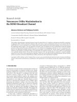
2
Figure 1: One iteration of the IEA method.
to Armijo’s rule, however, there is no test whether the step
size is too small, that is, t
0
is always considered large enough.
There exists a choice for the parameterisations φ
r
for
which
∇φ

r
(0), and thus ∇f
r
(0), is particularly simple to
compute. Let B
∈ R
K×K−1
denote an orthonormal basis of
the tangent space T
r
. Choose n such that the columns of
[
Bn
] constitute an orthonormal basis of
R
K
. Choose the
parameterisation φ
r
as follows:
φ
r
(μ) = r + Bμ + nδ(μ), (28)
where δ(μ) is chosen such that φ
r
(μ) ∈

E (correction step).
Then
∇φ

r
(0) = B
T
. (29)
As shown in Section 5.2, it is straightforward to find a basis
B. Combining (22), (23), (18), (28), and (29) yields
r
(n+1)
= r
(n)
+ tBB
T
∇u

r
(n)

+ nδ(t), (30)
with δ(t)
= δ(tB
T
∇u(r
(n)
). Accordingly, the update in rate
space is given by
r
(n+1)
−r
(n)
= tBB

T
∇u

r
(n)

+ nδ(t). (31)
The first summand in (31) is the orthogonal projection of
∇u(r
(n)
) on the tangent space. Based on this observation,
the proposed method can be interpreted as follows. First,
approximate the efficient set by its tangent space at r
(n)
.
Next, compute a gradient step, using this approximation.
Finally, make a correction step from the approximation back
to the efficient set, yielding r
(n+1)
. Based on the observation
that at each iteration, an approximation of the efficient set
is computed, the proposed method is denoted as iterative
efficient set approximation (IEA). For the case of K
= 2 users,
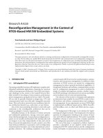
one iteration of the IEA method is illustrated in Figure 1.
Equation (19) defines an upper bound on the step size
t, which ensures that μ
(n+1)
stays within the domain of the
parameterisation φ

r
(n)
. The domain of the parameterisation
defined in (28) is defined implicitly by the requirement that
all entries of the resulting rate vector have to be positive, that
is,
U
r
=

μ : φ
r
(μ)  0

. (32)
In fact, the image and domain of the parameterisation
defined in (28) can be extended to also include rate vectors
with zero entries. From (32)and(30), an upper bound on
the step size t can then be derived by interpreting r
(n+1)
as a
function of t.Anupperboundont is given by the value of t
where the smallest entry in r
(n+1)
(t)isexactlyzero:
t :min
k
r
(n+1)
k

(t) = 0. (33)
Note that by (30), the upper bound
t depends on r
(n)
—thus
the validity range 0 <t<
t changes over

E, and it may get
small close to the boundary of E.
5.2. Correction Step. The most involved step is the computa-
tion of δ(μ
(n+1)
). Write r
(n+1)
as
r
(n+1)
= r + δn, (34)
with
r = r
(n)
+ Bμ
(n+1)
.Basedon(34), the correction step
can be interpreted as the projection of
r on E by computing
the intersection between E and the line
{r = r + xn, x ∈ R},
compare Figure 1. Assume that n

≥ 0 (the validity of this
assumption is verified at the end of this subsection). Then, δ
can be found by solving the following optimisation problem:
δ
= max
x,r
x s.t. r + xn ≤ r, r ∈ C. (35)
Note that (35) is a convex problem. In particular, it is
independent of the utility function u, that is, it is convex
regardless whether u is concave or not. Moreover, Slater’s
condition is satisfied, that is, strong duality holds. Accord-
ingly, (35) can be solved via Lagrange duality.
The Lagrangian of problem (35)isgivenby
L(x, r, λ)
= x + λ
T
(r −r −xn). (36)
Thedualfunctionfollowsas
g(λ)
= sup
x∈R
r∈C

x

1 −λ
T
n

+ λ

T
(r −r)

=
⎧
⎨
⎩
+∞, λ
T
n
/
=1,
max
r∈C
λ
T
(r −r), λ
T
n = 1.
(37)
Note that for λ
T
n = 1, again a weighted sum-rate
maximisation problem is to be solved. Recall from Section 4
that WsrMax can be efficiently solved as a convex problem in
the dual MAC.
Let r
∗
(λ) denote a maximiser of the weighted sum-rate
maximisation in (37)foragivenλ

∈ R
K
+
. The optimal dual
variable λ is found by solving
min
λ≥0
λ
T

r
∗
(λ) −r

s.t. λ
T
n = 1. (38)
6 EURASIP Journal on Advances in Signal Processing
According to Danskin’s Theorem [16], a subgradient (at λ)
of the cost function of problem (38)isgivenby(r
∗
(λ) −r).
If λ has equal entries, r
∗
(λ) is not unique [4]. Thus, the
subgradient is not unique, and the cost function is nondif-
ferentiable. Accordingly, the minimisation in (38)hastobe
carried out using any of the methods for nondifferentiable
convex optimisation, such as subgradient methods, cutting
plane methods, or the ellipsoid method [29]. All these

methods have in common that they generate iterates λ
(i)
(which converge to the optimal dual variable λ
∗
), and at each
iteration i, they require the computation of a subgradient
at λ
(i)
—which basically corresponds to solving a WsrMax
problem with weight λ
(i)
. In this work, an outer-linearisation
cutting plane method [16] is used to solve problem (38).
As strong duality holds, δ
= g(λ
∗
), and
r
(n+1)
= r + g(λ
∗
)n. (39)
From the optimal dual variable λ
∗
also follows the tan-
gent space at r
(n+1)
. Due to strong duality, r
(n+1)
maximises

L(x
∗
, r, λ
∗
)overC [16]. Accordingly, r
(n+1)
is a maximiser of
a WsrMax problem with weight λ
∗
. Recall that for WsrMax,
u(r)
= λ
T
r,with∇u(r) = λ. The corresponding composite
function f
r
is given by f
r
(μ) = λ
T
φ
r
(μ). As r
(n+1)
is a
maximiser of the WsrMax problem, it has to be a stationary
point (for this particular composite function, with λ
= λ
∗
).

From (24), it follows that:
∇

λ
∗

T
φ
r
(n+1)

(0) =∇φ
r
(n+1)
(0)λ
∗
= 0, (40)
thus
T
r
(n+1)
= null

λ
∗

T

. (41)
In other words, the basis B needed in the next iteration can

be obtained by computing an orthonormal basis of the null
space of (λ
∗
)
T
,whereλ
∗
is the optimal dual variable of the
current iteration. In addition, in the next iteration a unit
vector n
≥ 0 orthogonal to B is needed. From (41), it follows
that n (in the next iteration) is simply
n
=
λ
∗


λ
∗


2
. (42)
5.3. Time-Sharing Solutions. The algorithm described in
Sections 5.1 and 5.2 yields a stationary point r
∗
of problem
(12). The final step is the recovery of an optimal parameter
setup x

∗
P
from r
∗
. The complexity of the recovery step
depends on the location of r
∗
.Ifr
∗
/
∈R, then r
∗
lies in a
time-sharing region. Throughout this work, the term time-
sharing region denotes a subset of E whose elements are
only achievable by time-sharing. In case of time-sharing
optimality, the optimal parameter setup has to be found
by identifying a set of points in E
∩ R whose convex
combination yields r
∗
.
The recovery is based on the optimal dual variable of
the last correction step. If at least two entries in λ
∗
are
equal, time-sharing may be required. In the case of equal
entries in λ
∗
, there exist multiple rate vectors r ∈ R that

are maximisers of a WsrMax problem with weight λ
∗
[4],
and r
∗
is a convex combination of these points. In the
case that all entries in λ
∗
are equal, all permutations π are
optimal, resulting in K! points r
wsr
(λ
∗
, π). As a consequence,
enumerating all K! points first and then selecting the (at
most) K points that are actually required to implement r
∗
are
only feasible for small K.ForlargerK,anefficient method for
identifying a set of relevant points is provided in [30].
If no two entries in λ
∗
are equal, the optimum encoding
order π
∗
is uniquely defined, r
∗
= r
wsr
(λ

∗
, π
∗
), and Q
∗
maximises (λ
∗
)
T
r(Q, π
∗
), compare (13).
From an implementation viewpoint, entries in λ
∗
will
usually not be exactly equal, even if the theoretical solution
lies in a time-sharing region. As a result, time-sharing
between users is declared if the difference between weights
is below a certain threshold.
5.4. Coarse Projection. The proposed algorithm consists of
two nested loops: a gradient-based outer loop and an inner
loop for the correction step at each outer iteration. A
significant reduction in computational complexity can be
achieved if the required precision of the inner loop is adapted
to the outer loop. In fact, the convergence of the outer loop is
ensured by an increase in the cost function at each step, based
on condition (20). The inner iteration generates rate vectors
r
∗
(λ

(i)
) during convergence to λ
∗
.Ifr
∗
(λ
(i)
) fulfills condition
(20)andr
∗
(λ
(i)
) ∈

E, the projection of r on C is sufficiently
good to yield an ascent step on

E. In this case, the projection
is aborted, and the outer loop continues with
r
(n+1)
= r
∗

λ
(i)

. (43)
The resulting reduction in the number of inner iterations
comes at the price of an evaluation of the function u at

each inner iteration. As a result, the overall gain in terms
of complexity clearly depends on the cost associated with
evaluating u.
5.5. Boundary Points. So far, it has been assumed that at
the optimal solution r
∗
, all users have nonzero rate (i.e.,
r
∗
∈

E). If this assumption does not hold, the sequence
{r
(n)
} converges to a point on the boundary of E,compare
Section 5.6.Define
I(r)
=

k : r
k
= 0

. (44)
The boundary of E is given by
∂E
= E \

E =


r ∈ E : I(r)
/
=∅

. (45)
Observe that the boundary can be written as the union of K
sets ∂E
{k}
,with
∂E
{k}
=

r ∈ E : {k}⊂I(r)

. (46)
Finally, define a set E
{k}
by removing the kth entry (which
is zero) from all elements in ∂E
{k}
:
E
{k}
=

x ∈ R
K−1
: x


= r

, 
/
∈{k}, r ∈ ∂E
{k}

. (47)
EURASIP Journal on Advances in Signal Processing 7
Note that the resulting set E
{k}
is the efficient boundary of
a capacity region of a K
− 1userMIMOBC,withuser
k removed. It follows immediately that the interior E
{k}
is
again a differentiable manifold, now of dimension K
−1. The
boundary of E
{k}
can be decomposed in the same manner,
resulting in a set of K
−2 dimensional manifolds, and so on.
Accordingly, the set E
D
,withD ⊆{1, ,K} corresponds to
the efficient boundary of a capacity region of a K
−|D|user
MIMO BC, with users in D removed.

Accordingly, the general case is incorporated as follows.
Denote by A
={1, , K}\D the set of active users.
Only active users are considered in the optimisation, that is,
replace K by
|A| and let k be the index of the kth active user
in all steps of the algorithm. If the sequence
{r
(n)
} converges
to a point on the boundary of E
D
, the users with zero entries
in the rate vector are removed from A and assigned to D.
Initialise with A
={1, , K}, D = ∅,andr
(0)
∈

E.
With these modifications, the algorithm always operates on
differentiable manifolds

E
D
⊂ R
|A|
,withr  0 for all
r
∈


E
D
.
In practice, convergence to the boundary is detected
as follows. If the rate r
(n)
k
of an active user falls below a
threshold, and the projected utility gradient results in r
(n+1)
k
<
r
(n)
k
, the user is deactivated. The decision to deactivate a user
is based on the iterates and not on the limit point, thus the
modified algorithm may lead to suboptimal results if a user
is deactivated that actually has nonzero rate in the limit.
5.6. Convergence of the IEA Method. Concerning the conver-
gence of the IEA method, two cases can be distinguished.
In the first case, the sequence
{r
(n)
} converges to a point
in

E. In the second case, the sequence {r
(n)

} converges to
a point on the boundary of E. According to Section 5.5,
after removing the users with zero rate, the boundary itself
is a K
− 1 dimensional manifold with boundary, and the
algorithm converges in the interior or on the boundary of
this manifold. The argument continues until the dimension
of the manifold under consideration is 0. Thus, it suffices to
consider the convergence behaviour in the interior of E
D
,
which, from the perspective of the algorithm, is equivalent
to

E—anopensetequippedwithadifferentiable manifold
structure.
Accordingly, the IEA method is globally convergent if
convergence to a point r
∗
∈

E implies that r
∗
∈

E
is a stationary point. Convergence can be proved using
Zangwill’s global convergence theorem [26]. Not all param-
eterisations, however, yield a convergent method. For the
parameterisation defined in (28), global convergence (in the

sense of the global convergence theorem) is proved in [31].
A more intuitive (and less rigorous) discussion of the
convergence behaviour follows from considering the updates
μ
(n+1)
.Convergencetoapointr
∗
implies
μ
(n+1)
= t
(n)
∇f
r
(n)
(0) −→ 0. (48)
Now assume that r
∗
is not a stationary point. This implies
∇f
r
(n)
(0)
/
=0,foralln,which,by(48), implies t
(n)
→0. For
the parameterisation defined in (28),suchasequenceofstep
sizes results if the sequence of upper bounds
t(r

(n)
)converges
to zero. This behaviour, however, only occurs if the sequence
{r
(n)
} converges to a point on the boundary of E,which
contradicts the assumption that r
∗
∈

E.
The theoretical convergence results based on Zang-
will’s global convergence theorem assume infinite precision.
Theoretically, if
∇f
r
(n)
(0)
/
=0, it is always possible to find
astepsizet>0 such that (20)holds.Inapractical
implementation of the IEA method, the parameterisation is
evaluated numerically, in particular the correction step is a
numerical solution of a convex optimisation problem. Due
to the convexity of the correction problem, a high numerical
precision can be achieved. Still, the inherent finite precision
of the correction step sets a limit to the precision of the
overall algorithm. This property underlines the importance
of the coarse projection described in Section 5.4. The inner
loop needs a tight convergence criterion in order to yield a

high precision in cases where it is difficult to find an ascent
step. In cases where an ascent step is easily found, however,
it is not necessary to solve the problem to high precision.
The latter case is detected by the coarse projection. Also note
that the coarse projection does not impact the convergence
behaviour in a negative way. The global convergence ensures
that (theoretically) the algorithm does not get stuck at a
nonstationary point. The coarse projection only comes into
play if it is possible to move away from the current point.
It is clearly not guaranteed that a stationary point
r
∗
maximises utility. Due to the fact that the proposed
algorithm is an ascent method, however, r
∗
is a good solution
in the sense that given an initial value r
(0)
, utility is either
improved, or the algorithm converges at the first iteration
and stays at r
(0)
, in this case requiring no extra computations.
That is, any investment in terms of computational effort is
rewarded with a gain in utility.
6. Monotonic Optimisation
The gradient-based approach presented in Section 5 con-
verges to a stationary point of the optimisation problem, and
cannot guarantee convergence to global optimality, as it relies
on local information only.

The rate-space formulation (12) of the utility max-
imisation problem corresponds to the maximisation of a
monotonic function (the utility function u)overacompact
set in
R
K
+
(the capacity region C), and hence is a monotonic
optimisation problem [15], which can be solved to global
optimality.
A basic problem of monotonic optimisation is the
maximisation of a monotonic function over a compact
normal set [15]. A subset S of
R
K
+
is said to be normal in
R
K
+
(or briefly, normal), if x ∈ S, 0 ≤ y ≤ x ⇒ y ∈ S.The
capacity region C is normal: any rate vector r

that is smaller
thananachievableratevectorr is also achievable. Thus, C
is a compact normal set and the rate-space problem (12)isa
basic problem of monotonic optimisation.
6.1. Polyblock Algorithm. The basic algorithm for solving
monotonic optimisation problems is the so-called polyblock
8 EURASIP Journal on Advances in Signal Processing

algorithm. A polyblock is simply the union of a finite number
of hyperrectangles in
R
K
+
. Given a discrete set V ⊂ R
K
+
,a
polyblock P (V)isdefinedas
P (V)
=

v∈V

r ∈ R
K
+
, r ≤ v

. (49)
The set V contains the vertices of the polyblock P (V).
Due to the fact that C is a compact normal subset of
R
K
+
,
there exists a set V
(0)
such that C ⊆ P (V

(0)
). Moreover,
starting with n
= 0, either C = P (V
(n)
) or there exists a
discrete set V
(n+1)
⊂ R
K
+
such that
C
⊆ P

V
(n+1)

⊂ P

V
(n)

. (50)
In other words, the polyblocks P (V
(n)
) represent an itera-
tively refined outer approximation of the capacity region.
Consider the problem of maximising utility over the
polyblock P (V

(n)
):
max
r∈P (V
(n)
)
u(r). (51)
Let
ˇ
r
(n)
denote a maximiser of problem (51), Due to the
monotonicity of u,
ˇ
r
(n)
∈ V
(n)
, that is, the maximum of
a monotonic function over a polyblock is attained on one
of the vertices [15]. Due to the fact that the vertex set of a
polyblock is discrete, problem (51) can be solved to global
optimality by searching over all v
∈ V
(n)
.
If
ˇ
r
(n)

∈ E, the globally optimal rate vector is found.
In general, however,
ˇ
r
(n)
will lie outside the capacity region,
due to the fact that the polyblock represents an outer
approximation. Denote by y
(n)
∈ E the intersection between
E and the line segment connecting the origin with
ˇ
r
(n)
.Let
r
(n)
denote the best intersection point computed so far, that
is,
r
(n)
= y
(
∗
)
, 
∗
= arg max
∈{1, ,n}
u


y
()

. (52)
Moreover, let u
∗
denote the global maximum of (12). It
follows that
u

r
(n)

≤ u
∗
≤ u

ˇ
r
(n)

. (53)
Intuitively, as the outer approximation of C by a polyblock is
refined at each step, u(
ˇ
r
(n)
) eventually converges to u
∗

.Due
to the continuity of u, this convergence also holds for
r
(n)
,
that is,
r
(n)
converges to a global maximiser of u. See [15]for
a rigorous proof. According to (53), an
-optimal solution is
found if u(
r
(n)
) ≥ u(
ˇ
r
(n)
) −.
One possible method to construct a sequence of poly-
blocks P (V
(n)
) that satisfies (50) is as follows [15]. Define
K(r)
=

x ∈ R
K
+
: x

k
>r
k
, k
/
∈I(r)

, (54)
with I(r)asdefinedin(44). Clearly,
r
(n)
∈ E implies
K(
r
(n)
) ∩ C = ∅.Thus,K(r
(n)
)canberemovedfrom
P (V
(n)
) without removing any achievable rate vector. More-
over, if
ˇ
r
(n)
/
∈E,
K

r

(n)

∩P

V
(n)

⊃

ˇ
r
(n)

⊃ ∅, (55)
thus by removing K(
r
(n)
), a tighter approximation results.
Finally, P (V
(n)
) \ K(r
(n)
)isagainapolyblock[15]. To
summarise, the desired rule for constructing a sequence of
polyblocks that satisfies (50)is
P

V
(n+1)


=
P

V
(n)

\K

r
(n)

. (56)
The rules for computing the corresponding vertex set V
(n+1)
are provided in [15].
6.2. Intersection with E. If the polyblock algorithm is applied
to the rate-space problem (12), the only step in the algorithm
in which the intricate properties of the capacity region
C come into play is the computation of the intersection
between E and the line connecting the origin with
ˇ
r
(n)
.
Comparing the correction step of the IEA algorithm from
Section 5.2 with the computation of the intersection point,
it turns out that both operations are almost identical, only
the line whose intersection with E is computed is different.
As a result, the Lagrangian-based algorithm from Section 5.2
can also be used to compute the intersection point, by setting

r =
ˇ
r
(n)
, n =
ˇ
r
(n)
. (57)
In Section 5, it was stated that the most complex step in
each iteration of the IEA method is the correction step.
Similar results hold for the polyblock algorithm. At each
iteration, the main complexity lies in the computation of
the intersection point. Due to the similarity between IEA’s
correction step and the computation of the intersection
point in the polyblock algorithm, the complexity of both
approaches can be compared by comparing the number of
gradient iterations with the number of polyblocks generated
until a sufficiently tight outer approximation is found. The
convergence properties of the polyblock algorithm are only
asymptotic [15]—thus, a relatively high complexity of the
polyblock algorithm can be expected. This expectation is
confirmed by simulation results; see Section 8.
6.3. Implementation Issues. The presentation of the poly-
block algorithm in Section 6.1 closely follows [15]. In this
basic version, simulations showed very slow convergence
of the algorithm, due to the fact that close to regions on
the boundary where at least on rate gets close to zero, a
large number of iterations are needed until a significant
refinement results. A similar behaviour is reported in [32].

Following [32], the convergence speed of the algorithm can
be significantly improved by modifying the direction of the
line whose intersection with E defines the next iterate y
(n)
.
Computationally, this is achieved by setting n
=
ˇ
r
(n)
+ a,
a
∈ R
K
+
in the algorithm from Section 5.2.
An initial vertex set V
(0)
can be determined as follows.
Define a rate vector v
∈ R
K
+
whose kth entry v
k
corresponds
to the maximum rate achievable for user k.Then,V
(0)
=
{

ωv} with ω ≥ 1 defines a polyblock that contains the
capacity region.
EURASIP Journal on Advances in Signal Processing 9
7. Dual Decomposition
For concave utilities, a dual approach to solve the utility
maximisation problem in the MIMO BC was recently
proposed in [14]. The algorithm in [14] represents an
application of the dual decomposition [10]. Similar to the
gradient-based method developed in Section 5, the solution
is found in two steps. First, an optimal rate vector r
∗
is
found by operating in the rate space; second, the optimal
parameters are derived from r
∗
.
In the first step, problem (12) is modified by introducing
additional variables:
max
r,s
u(s)s.t.0 ≤ s ≤ r, r ∈ C. (58)
The dual function is chosen as
g(λ)
= max
s≥0
u(s) −λ
T
s
  
g

A
(λ)
+max
r∈C
λ
T
r
  
g
P
(λ)
. (59)
Evaluating the dual function at λ results in two decoupled
subproblems, computing g
A
(λ)andg
P
(λ) by maximising
over the primal variables s and r, respectively. Computing
g
P
(λ) is again a WsrMax problem.
The optimal dual variable is found by minimising the
dual function with respect to λ. The dual function is always
convex, regardless of the properties of the utility function u
[16].
If the utility function u is concave, strong duality holds,
and the optimal primal solution r
∗
can be recovered from

the dual solution by employing standard methods for primal
recovery, as in [14]. Also, for concave u,efficient methods
exist to find a set of corner points that implement r
∗
in the
case of time-sharing optimality [30].
Being entirely based on Lagrange duality, a nonconcave
utility poses significant problems to the dual decomposition.
Most importantly, recovering an optimal primal solution
(r
∗
, s
∗
) from the dual solution is, in general, no longer
possible. Moreover, the schemes for recovering all parameters
x
P
of a time-sharing solution rely on strong duality to hold
[30]. For nonconcave u,however,strongdualitycannotbe
assumed to hold. In fact, simulation results in Section 8 show
a significant duality gap in the scenario under consideration.
As a result, for nonconcave u, the following heuristic is
used to obtain a primal feasible solution (
r,s). Given the
optimal dual variable λ
∗
, choose r = r
wsr
(λ
∗

, π
∗
), where
π
∗
is any optimal encoding order. Moreover, let s = r.An
upper bound on the loss incurred by this approximation
follows immediately from weak duality. Let u
∗
denote the
(unknown) maximum utility value. By weak duality, g(λ
∗
) ≥
u
∗
,thusu
∗
−u(r) ≤ g(λ
∗
)−u(r). The tightness of this bound
clearly depends on the duality gap, which is not known.
8. Simulation Results
Utility maximisation in a K = 3 user Gaussian MIMO
broadcast channel with N
= 6 transmit antennas and M
k
=
2 receive antennas per user is simulated. The channels H
k
are i.i.d. unit-variance complex Gaussian. Furthermore, the

12345
γ
0
0.2
0.4
0.6
0.8
1
Average utility
IEA
DD
SR
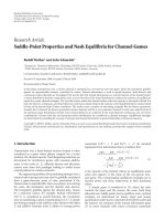
Figure 2: Average utility (concave utilities).
maximum transmit power is P
tr
= 10. To obtain rates
in Kbps, rates are multiplied by a bandwidth factor W
=
60 kHz.
In the simulations, the utility u is given by a weighted
sum of the users’ utilities u
k
:
u(r)
=
K

k=1
w
k

u
k

r
k

. (60)
The IEA method always uses a sum-rate maximising rate
vector as initial point r
(0)
. The results are averaged over 1000
channel realisations.
Two d ifferent models for the users’ utilities u
k
are
considered: a concave logarithmic utility and a nonconcave
sigmoidal utility.
8.1. Concave Utility. The logarithmic utility function is
defined as
u
k

r
k

=
b ln

1+c
−1

r
k

, (61)
with constants b, c. In the simulations, c
= 40 Kbps and b
is chosen such that u
k
(1000 Kbps) = 1. The weights w
k
are
chosen according to the following scheme:
ω
=

1 γγ
2

,
w
=
ω
ω
1
,
(62)
with γ
∈{1, ,5}. Figure 2 shows the average utility for the
case of logarithmic utility functions. What is shown is the
average utility for the gradient-based approach (IEA), for the

dual decomposition (DD), and, as a reference, the average
utility obtained by using for transmission the sum-rate (SR)
maximising rate vector that corresponds to encoding order
π
= [
123
].
10 EURASIP Journal on Advances in Signal Processing
0 200 400 600 800
Rate (Kbps)
0
0.2
0.4
0.6
0.8
1
Utility
a = 0.01
a
= 0.02
a
= 0.05
Figure 3: Sigmoid utility function, b = 400 Kbps.
Due to the fact that the utility maximisation problem
is convex, both IEA and DD achieve identical performance.
Moreover, for identical weights w
k
, cross-layer optimisation
does not provide a significant gain compared to the sum-
rate maximising strategy. The larger the difference between

the users’ weights, the larger the gain achieved by cross-layer
optimisation. This result is not surprising, as for asymmetric
setups, it is more important to adapt the physical layer to the
characteristics of the upper layers. Moreover, the decay of the
logarithmic utility function is rather moderate around the
optimal rate vector, therefore a maximiser of the weighted
sum-rate is almost optimal for equal weights.
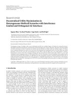
8.2. Nonconcave Utility. The nonconcave utility model is
adopted from [8]. For each user k, the following sigmoidal
utility function is used:
u
k

r
k

=
c
k

1
1+exp

−a
k

r
k
−b
k


+ d
k

, (63)
where c
k
and d
k
are used to normalise u
k
such that u
k
(0) = 0
and u
k
(∞) = 1. The steepness of the transition between the
minimum value and the maximum value is controlled by
the parameter a
k
,whereasb
k
determines the inflection point
of the utility curve (cf. Figure 3). In the simulations, a
k
=
a Kbps
−1
,anda is varied in a range between 0.01 and 0.05,
modelling different degrees of elasticity of the applications.

For each channel realisation, the constant b
k
of each user
is chosen randomly in the interval [300 Kbps, 500 Kbps]
according to a uniform distribution. Choosing the b
k
randomly can be understood as a model for fluctuations in
the data rate requirements of the users over time, that is,
transmission of a video source with varying scene activity.
All users have equal weight w
k
= 1/K.
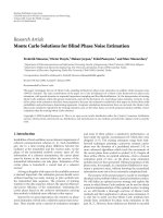
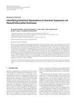
Figure 4 shows the average utility for the case of sig-
moidal utility functions. What is shown is the average
0.01 0.02 0.03 0.04 0.05
a
0
0.2
0.4
0.6
0.8
1
Average utility
IEA
PB
DD
SR
DUB
Figure 4: Average utility (sigmoidal utilities).
utility for the gradient-based approach (IEA), the polyblock

algorithm (PB), the dual decomposition (DD), and the
sum-rate (SR) maximising rate vector. In addition, the
average minimum value of the dual function in the dual
decomposition approach is shown (DUB). The PB algorithm
finds the global maximum for each realisation. As a result,
the PB curve gives the maximum achievable average utility.
In terms of average utility, the performance of the IEA
method is close to optimal. It can be concluded that for the
system setup under consideration, the IEA method succeeds
in finding a stationary point which is identical or close to
the global maximum for most realisations. In contrast, the
dual decomposition-based method does not find a good
rate vector in most cases. The poor performance of the
computationally simple SR strategy emphasises the need
for cross-layer optimisation. In particular, the performance
gain achieved by both PB and IEA increases with a. This
behaviour can be explained as follows. With increasing a,
the interval in which the utility function makes a transition
from small to large values becomes smaller. Therefore, it
becomes more and more important to adapt the physical
layer parameters to the utility characteristics.
The results in Figure 4 also show that the dual upper
bound (DUB) obtained from the dual decomposition is
rather loose. This implies that there is a significant duality
gap in most cases.
8.3. Complexity Analysis. If average utility is the only figure
of merit, the polyblock algorithm is obviously superior
to all other approaches. From a practical viewpoint, a
second metric of interest is the computational complexity
of the different approaches. In the following, the utility-

complexity tradeoffs provided by the different approaches
are investigated. All results are for the case of sigmoidal utility
functions.
EURASIP Journal on Advances in Signal Processing 11
0 5 10 15 20 25 30
Iterations
0.25
0.3
0.35
0.4
0.45
0.5
0.55
0.6
0.65
Average utility
Figure 5: Average utility versus number of iterations, IEA method.
In Figure 5, average utility is plotted versus the number of
iteration for the IEA method. The plot shows three graphs,
corresponding to three different values of the steepness
parameter a: a
∈{0.01, 0.03, 0.05}. Note that the rightmost
points of each graph correspond to the average utility
value in Figure 4. Only the gradient-based outer iterations
defined in (21)–(23) are counted, the inner iterations in the
correction step are neglected. Figure 5 shows that the IEA
method needs between five and 10 iterations to get close to
the maximum achieved utility value.
In Figure 6, average utility is plotted versus the number of
iteration for the polyblock algorithm. The plot shows three

pairs of graphs, with each pair corresponding to a different
value of the steepness parameter a: a
∈{0.01, 0.03, 0.05}.
Each pair consists of two graphs, one showing the average of
the current best utility value u(
r
(n)
) (CBV, dash-dotted line),
the other showing the average of the upper bound u(
ˇ
r
(n)
)
(UB, solid line). Depending on the parameter a,between
50 to 75 iterations are needed until the current best value is
close to the global maximum. Recall from Section 6.1 that the
convergence criterion for the PB algorithm is based on the
difference between u(
r
(n)
)andu(
ˇ
r
(n)
). Figure 6 shows that a
large number of iterations may be required until convergence
is declared, due to the relatively slow convergence of the
upper bound.
In both Figures 5 and 6, the number of inner iterations
required in the correction step and the computation of the

intersection point, respectively, are not counted. In each
inner iteration, a WsrMax problem is solved. Moreover, a
WsrMax problem is also solved at each iteration of the
dual decomposition. Accordingly, all three approaches can
be compared based on the number of calls to the WsrMax
subroutine. Figure 7 shows the average utility that is achieved
if the maximum number of calls to WsrMax is limited
to a value maxcall, with maxcall increased in steps of 10
calls. Again, three groups of graphs are shown, each group
corresponding to a value of a,witha
∈{0.01, 0.03, 0.05}.
As an example, the results show that the dual decomposition
0 50 100 150
Iterations
0.2
0.3
0.4
0.5
0.6
0.7
0.8
0.9
1
Average utility
CBV
UB
Figure 6: Average utility versus number of iterations, PB algorithm.
needs between 10 and 20 iterations until convergence (to a
clearly suboptimal solution). Of particular interest are the
cross-over points between IEA method and PB algorithm.

For a
= 0.05, the cross-over point is at maxcall = 300, that
is, only if more than a maximum of 300 calls to WsrMax are
feasible does the PB algorithm outperform the IEA method.
Moreover, for small values of maxcall, the IEA method
provides significantly larger average utility.
9. Conclusions
Two methods for solving the nonconcave utility maximisa-
tion problem in the MIMO broadcast channel are proposed:
a gradient-based method that converges to a locally optimal
solution, and an approach based on monotonic optimisation
that yields the global optimum. Due to the structure of
the MIMO BC capacity region, a direct optimisation in
terms of the physical layer parameters transmit covariance
matrices and encoding order is not feasible. Thus, as an
intermediate step, both methods first determine an optimal
rate vector. The optimal physical layer parameter setup,
which may include a time-sharing solution, is then obtained
from this rate vector. For both methods, the formulation of
the utility maximisation problem in the rate space represents
a key step. The IEA method exploits the differentiable
manifold structure of the efficient boundary of the capacity
region, while the polyblock algorithm relies on the fact that
maximising utility over the set of achievable rate vectors
represents a monotonic optimisation problem.
The polyblock algorithm provides globally optimal per-
formance, at the price of a relatively high computational
complexity. From a practical viewpoint, the proposed IEA
method provides an attractive tradeoff between utility per-
formance and computational complexity. In the simulation

setup used in this work, the average utility achieved by
12 EURASIP Journal on Advances in Signal Processing
10
1
10
2
10
3
10
4
10
5
maxcall
0
0.1
0.2
0.3
0.4
0.5
0.6
0.7
Average utility
IEA
PB
DD
Figure 7: Average utility versus maximum number of WsrMax
calls.
the IEA method is close to optimal, at significantly lower
complexity than the polyblock algorithm.
Throughout this work, it is assumed that users’ rates are

the only relevant performance metrics of the physical layer,
implying that rate cannot be traded for delay and reliability.
In a more general setup, more than one performance metric
per user may be required to characterise the physical layer,
corresponding to a utility function that is a function of all
these metrics [7]. Concerning the results presented in this
work, this would clearly impact the mapping from physical
layer parameters to set of achievable performance vectors.
The methods proposed in this work, however, would still
be applicable, provided the structural assumptions of each
method are still met (i.e., the utility function is monotone in
all physical layer metrics, the set of achievable performance
vectors is compact and, in case of the IEA method, can be
equipped with a differentiable manifold structure). While
the capacity region is convex, it is not clear whether a
generalised achievable region can still be assumed to be
convex. This observation represents a further motivation
for an optimisation framework that does not rely on the
assumption of convexity.
References
[1] G. Caire and S. Shamai, “On the achievable throughput of a
multiantenna Gaussian broadcast channel,” IEEE Transactions
on Information Theory, vol. 49, no. 7, pp. 1691–1706, 2003.
[2]P.ViswanathandD.N.C.Tse,“Sumcapacityofthevector
Gaussian broadcast channel and uplink-downlink duality,”
IEEE Transactions on Information Theory,vol.49,no.8,pp.
1912–1921, 2003.
[3] S. Vishwanath, N. Jindal, and A. Goldsmith, “Duality,
achievable rates, and sum-rate capacity of Gaussian MIMO
broadcast channels,” IEEE Transactions on Information Theory,

vol. 49, no. 10, pp. 2658–2668, 2003.
[4] H. Viswanathan, S. Venkatesan, and H. Huang, “Down-
link capacity evaluation of cellular networks with known-
interference cancellation,” IEEE Journal on Selected Areas in
Communications, vol. 21, no. 5, pp. 802–811, 2003.
[5] N. Jindal and A. Goldsmith, “Dirty-paper coding versus
TDMA for MIMO broadcast channels,” IEEE Transactions on
Information Theory, vol. 51, no. 5, pp. 1783–1794, 2005.
[6] H. Weingarten, Y. Steinberg, and S. Shamai, “The capacity
region of the Gaussian multiple-input multiple-output broad-
cast channel,” IEEE Transactions on Information Theory, vol.
52, no. 9, pp. 3936–3964, 2006.
[7] S. Shenker, “Fundamental design issues for the future Inter-
net,” IEEE Journal on Selected Areas in Communications, vol.
13, no. 7, pp. 1176–1188, 1995.
[8] J W. Lee, R. R. Mazumdar, and N. B. Shroff,“Non-convex
optimization and rate control for multi-class services in the
Internet,” IEEE/ACM Transactions on Networking, vol. 13, no.
4, pp. 827–840, 2005.
[9] M. Fazel and M. Chiang, “Network utility maximization
with nonconcave utilities using sum-of-squares method,” in
Proceedings of the 44th IEEE Conference on Decision and
Control, and the European Control Conference (CDC-ECC ’05),
pp. 1867–1874, Seville, Spain, December 2005.
[10]M.Chiang,S.H.Low,A.R.Calderbank,andJ.C.Doyle,
“Layering as optimization decomposition: a mathematical
theory of network architectures,” Proceedings of the IEEE, vol.
95, no. 1, pp. 255–312, 2007.
[11] F. Kelly, “Charging and rate control for elastic traffic,”
European Transactions on Telecommunications,vol.8,no.1,pp.

33–37, 1997.
[12] X. Lin, N. B. Shroff, and R. Srikant, “A tutorial on cross-layer
optimization in wireless networks,” IEEE Journal on Selected
Areas in Communications, vol. 24, no. 8, pp. 1452–1463, 2006.
[13] S. Stanczak, M. Wiczanowski, and H. Boche, Resource Allo-
cation in Wireless Networks: Theory and Algorithms,Lecture
Notes in Computer Science 4000, Springer, Berlin, Germany,
2006.
[14] J. Liu, Y. T. Hou, and H. D. and Sherali, “Routing and power
allocation for MIMO-based ad hoc networks with dirty paper
coding,” IEEE International Conference on Communications
(ICC ’08), pp. 2859–2864, May 2008.
[15] H. Tuy, “Monotonic optimization: problems and solution
approaches,” SIAM Journal on Optimization,vol.11,no.2,pp.
464–494, 2000.
[16] D. Bertsekas, A. Nedic, and A. Ozdaglar, Convex Analysis and
Optimization, Athena Scientific, Belmont, Mass, USA, 2003.
[17] H. Schwarz, D. Marpe, and T. Wiegand, “Overview of the
scalable H.264/MPEG4-AVC extension,” in Proceedings of the
IEEE International Conference on Image Processing (ICIP ’06),
pp. 161–164, Atlanta, Ga, USA, October 2006.
[18] D. N. C. Tse and S. V. Hanly, “Multiaccess fading channels—
part I: polymatroid structure, optimal resource allocation
and throughput capacities,” IEEE Transactions on Information
Theory, vol. 44, no. 7, pp. 2796–2815, 1998.
[19] M. Kobayashi and G. Caire, “An iterative water-filling algo-
rithm for maximum weighted sum-rate of Gaussian MIMO-
BC,” IEEE Journal on Selected Areas in Communications, vol.
24, no. 8, pp. 1640–1646, 2006.
[20] R. B

¨
ohnke and K D. Kammeyer, “Weighted sum rate maxi-
mization for the MIMO-downlink using a projected conjugate
EURASIP Journal on Advances in Signal Processing 13
gradient algorithm,” in Proceedings of the International Work-
shop on Cross Layer Design (IWCLD ’07), pp. 82–85, Jinan,
China, September 2007.
[21] D. G. Luenberger, “The gradient projection method along
geodesics,” Management Science, vol. 18, no. 11, pp. 620–631,
1972.
[22] D. Gabay, “Minimizing a differentiable function over a
differential manifold,” Journal of Optimization Theory and
Applications, vol. 37, no. 2, pp. 177–219, 1982.
[23] J. H. Manton, “Optimization algorithms exploiting unitary
constraints,” IEEE Transactions on Signal Processing, vol. 50,
no. 3, pp. 635–650, 2002.
[24] J. B. Rosen, “The gradient projection method for nonlinear
programming—part II: nonlinear constraints,” SIAM Journal
on Applied Mathematics, vol. 9, no. 4, pp. 514–553, 1961.
[25] W. Boothby, An Introduction to Differentiable Manifolds and
Riemannian Geometr y, Academic Press, New York, NY, USA,
1975.
[26] W. Zangwill, Nonlinear Programming: A Unified Approach,
Prentice-Hall, Englewood Cliffs, NJ, USA, 1969.
[27] J. H. Manton, “On the various generalisations of optimisation
algorithms to manifolds,” in Proceedings of the 6th Interna-
tional Symposium on Mathematical Theory of Networks and
Systems (MTNS ’04), Leuven, Belgium, July 2004.
[28] D. G. Luenberger, Linear and Nonlinear Programming,
Addison-Wesley, Reading, Mass, USA, 2nd edition, 1984.

[29] J L. Goffin and J P. Vial, “Convex nondifferentiable opti-
mization: a survey focussed on the analytic center cutting
plane method,” Tech. Rep. 99.02, Logilab, Geneva, Switzer-
land, 1999.
[30] J. Brehmer, Q. Bai, and W. Utschick, “Time-sharing solutions
in MIMO broadcast channel utility maximization,” in Pro-
ceedings of the International ITG Workshop on Smart Antennas
(WSA ’08), pp. 153–156, Vienna, Austria, February 2008.
[31] M. Riemensberger and W. Utschick, “Gradient descent on
differentiable manifolds,” Tech. Rep. MSV-2008-1, Technische
Universit
¨
at M
¨
unchen, Munich, Germany, 2008.
[32] H. Tuy, F. Al-Khayyal, and P. Thach, “Monotonic optimiza-
tion: branch and cut methods,” in Essays and Surveys in Global
Optimization,C.Audet,P.Hansen,andG.Savard,Eds.,pp.
39–78, Springer, New York, NY, USA, 2005.