Báo cáo hóa học: " Research Article Robust Adaptive Modified Newton Algorithm for Generalized Eigendecomposition and Its Application" pdf

Hindawi Publishing Corporation
EURASIP Journal on Advances in Signal Processing
Volume 2007, Article ID 38341, 10 pages
doi:10.1155/2007/38341
Research Article
Robust Adaptive Modified Newton Algorithm for Generalized
Eigendecomposition and Its Application
Jian Yang, Feng Yang, Hong-Sheng Xi, Wei Guo, and Yanmin Sheng
Laboratory of Network Communication System a nd Control, Department of Automation, University of Sci ence
and Technology of China, Hefei, Anhui 230027, China
Received 1 October 2006; Revised 13 February 2007; Accepted 16 April 2007
Recommended by Nicola Mastronardi
We propose a robust adaptive algorithm for generalized eigendecomposition problems that arise in modern signal processing
applications. To that extent, the generalized eigendecomposition problem is reinterpreted as an unconstrained nonlinear opti-
mization problem. Starting from the proposed cost function and making use of an approximation of the Hessian matrix, a robust
modified Newton algorithm is derived. A rigorous analysis of its convergence properties is presented by using stochastic approxi-
mation theory. We also apply this theory to solve the signal reception problem of multicarrier DS-CDMA to illustrate its practical
application. The simulation results show that the proposed algorithm has fast convergence and excellent tracking capability, which
are important in a practical time-varying communication environment.
Copyright © 2007 Jian Yang et al. This is an open access article distributed under the Creative Commons Attribution License,
which permits unrestricted use, distribution, and reproduction in any medium, provided the original work is properly cited.
1. INTRODUCTION
Generalized eigendecomposition has extensive applications
in modern signal processing areas, for example, pattern
recognition [1, 2], and signal processing for wireless com-
munications [3, 4]. Many efficient adaptive algorithms have
been proposed for principal component analysis [5–7],
which is a special case of generalized eigendecomposition.
However, developing efficient adaptive algorithms for gen-
eralized eigendecomposition has not been addressed so far.
This paper aims to propose a novel adaptive online algorithm

for generalized eigendecomposition.
Consider the matrix pencil (R
y
, R
x
), where R
y
and R
x
are
M
× M Hermitian and positive-definite matrices. A scalar λ
and M
× 1vectorw that satisfy [8, 9]
R
y
w = λR
x
w (1)
are called the generalized eigenvalue and corresponding gen-
eralized eigenvector of matrix pencil (R
y
, R
x
), respectively. In
this paper, we are interested in finding the generalized eigen-
vector corresponding to the largest eigenvalue.
Many numerical methods have been presented for
the generalized eigendecomposition problem [8]. However,
these methods are inefficient in a nonstationary signal envi-

ronment, since they are computationally intensive and be-
long to the class of batch processing methods. For practi-
cal signal processing applications, a n adaptive online algo-
rithm is preferred, especially in a nonstationary signal envi-
ronment. Chatterjee et al. have presented an online gener-
alized eigendecomposition algorithm for linear discriminant
analysis (LDA) [10]. However, this algorithm as well as those
in [11, 12] are based on the g radient method, and their per-
formance is largely determined by the step size, which is diffi-
cult to select in a practical application. To overcome these dif-
ficulties, Rao et al. apply a fixed-point algorithm to solve the
generalized eigendecomposition problem [13]. The result-
ing RLS-like algorithm is proven to be more computation-
ally feasible and faster than most of the gradient methods.
Recently, by using the recursive least-square learning rule,
Yang et al. develop fast adaptive algorithms for the gener-
alized eigendecomposition problem [14]. Besides RLS tech-
niques, the Newton method is also a well-known powerful
technique in the area of optimization. By constructing a cost
function based on the penalty function method, Mathew and
Reddy develop a quasi-Newton adaptive algorithm for es-
timating the generalized eigenvector corresponding to the
smallest generalized eigenvalue [9]. However, this method
suffers from the difficulty of selecting an appropriate penalty
factor, which requires its priori information of the covariance
matrices, which is unavailable in most applications. As a re-
sult, this will affect the learning performance. In addition, for
2 EURASIP Journal on Advances in Signal Processing
many applications, the generalized eigenvector correspond-
ing to the largest eigenvalue is desired.

In this paper, motivated by the work of Mathew and
Reddy [9], we develop an efficient adaptive modified Newton
algorithm to track the adaptive principal generalized eigen-
vector. The basic idea is that we reformulate the general-
ized eigendecomposition problem as minimizing an uncon-
strained nonquadra tic cost function that has a unique global
minimum and no other local minima, and then apply an ap-
propriate Hessian matrix approximation to derive an adap-
tive modified Newton algorithm. The resulting algorithm is
numerically robust no matter whether it is implemented with
infinite or finite precision. We also illustrate its application
by using it to solve an adaptive signal reception problem in a
multicarrier DS-CDMA (MC-DS-CDMA) system [15].
The rest of the paper is organized as follows. In Section 2,
we formulate the adaptive signal reception problem in an
MC-DS-CDMA system as the principal generalized eigenvec-
tor estimation problem, to show the importance of the gener-
alized eigendecomposition technique. In Section 3, the gen-
eralized eigendecomposition problem is reinterpreted as a
nonlinear optimization problem, and a robust adaptive mod-
ified Newton algorithm is developed to estimate the princi-
pal generalized eigenvector. The convergence property of the
proposed algorithm is also discussed. In Section 4,wepresent
numerical simulation results to show the performance of the
proposed algorithm. Conclusions are drawn in Section 5.
2. GENERALIZED EIGENDECOMPOSITION
APPLICATION
In this section, we show that it is possible to formulate the
signal reception problem in a multicarrier DS-CDMA system
[16] as a generalized eigendecomposition problem.

2.1. Signal model of MC-DS-CDMA system
Consider an MC-DS-CDMA system with K simultaneous
users. Each one uses the same M carriers. The kth user, for
1
≤ k ≤ K, generates a data sequence:
b
(k)
=

, b
(k)
0
, b
(k)
1
, b
(k)
2
,

(2)
with a symbol interval of T seconds. We assume that the data
symbols b
(k)
j
are independent variables with E[b
(k)
j
] = 0and
E[

|b
(k)
j
|] = 1.
The kth user is provided a randomly generated signature
sequence:
a
(k)
=

, a
(k)
0
, a
(k)
1
, , a
(k)
G
−1
,

,(3)
where G is the spreading gain and the elements a
(k)
i
are mod-
elled as independent and identically distributed (i.i.d.) ran-
dom variables such that Pr(a
(k)

i
=−1) = Pr(a
(k)
i
= 1) = 1/2.
The sequence a
(k)
is used to spectrally spread the data sym-
bols to form the signal [15]
a
k
(t) =
∞

i=−∞
b
(k)
i/G
a
(k)
i
ψ

t − iT
c

,(4)
where
x denotes the largest integer less than or equal to x,
the chip interval T

c
is given by T
c
= T/G, G is the number
of chips per symbol interval, and ψ(t) is the common chip
waveform for all signals. We assume that the chip waveform
ψ(t) is bandlimited, such as the square-root raised-cosine
pulse [17], and nor malized so that

∞
−∞
ψ(t)
2
dt = T
c
.
Assume a slowly time-varying frequency-selective Ray-
leigh fading channel. Following the approach [16], by suit-
ably choosing M and the bandwidth of ψ(t), we can assume
that each carrier experiences slowly varying flat fading. Then,
the received signal in complex form is given by [18]
r(t)
=
K

k=1
M

m=1


2P
k
α
k,m
e
jω
m
t
·

∞

i=−∞
b
(k)
i/G
a
(k)
i
ψ

t − iT
c
− τ
k


+ n(t),
(5)
where ω

m
is the frequency of the mth carrier, α
k,m
accounts
for the overall effects of phase shifts and fading for the mth
carrier of the kth user, P
k
and τ
k
∈ [0, T) represent the power
for each carrier of the transmitted signal and the delay of the
kth user signal, respectively, and n(t) denotes additive white
Gaussian noise.
Without loss of generality, throughout the paper we will
consider the signal from the first user as the desired signal
and the signals from all other users as interfering signals. As-
sume that synchronization has been achieved with the trans-
mitted signal of the desired user. Therefore, the delay of the
desired signal τ
1
can be taken to be zero. In order to avoid
interchip interference for the desired signal when it is chip-
synchronous, the waveform is chosen to satisfy the Nyquist
criterion. Then the input signal to the first PN correlator (fin-
ger) associated with the mth carrier is written as
x
m
[g] =
1
T

c

∞
−∞
r(t)ψ
∗

t − gT
c

e
−jω
m
t
dt
=

2P
1
α
1,m
b
(1)
g/G
a
(1)
g
+
K


k=2
i
k,m
[g]+n
m
[g],
(6)
where g is the chip index, n
m
[g] denotes the component due
to AWGN, and
i
k,m
[g] =

2P
k
α
k,m
∞

i=−∞
b
(k)
i/G
a
(k)
i
R
ψ


(g − i)T
c
− τ
k

(7)
is the component due to the kth user signal, 2
≤ k ≤ K.The
function R
ψ
(·) is the autocorrelation of the chip waveform
defined by
R
ψ
(t) =
1
T
c

∞
−∞
ψ(s)ψ
∗
(s − t)ds. (8)
The input signal vector can be written as
x[g]
=

x

1
[g], x
2
[g], , x
m
[g]

T
= h
1
b
(1)
g/G
a
(1)
g
+
K

k=2
h
k
∞

i=−∞
b
(k)
i/G
a
(k)

i
· R
ψ

(g − i)T
c
− τ
k

+ n[g],
(9)
Jian Yang et al. 3
where h
k
= [

2P
k
α
k,1
, ,

2P
k
α
k,m
]
T
,1 ≤ k ≤ K,and
n[g]

= [n
1
[g], n
2
[g], , n
M
[g]]
T
is a zero-mean Gaussian
random vector with covariance σ
2
I.
Then, the output signal of the first PN correlator to ex-
tract the signal at the mth carrier can be w ritten as
y
m
[n] =
1
√
G
G−1

l=0
a
(1)
l+Gn
x
m
[Gn + l] (10)
and the output signal vector can be expressed as

y[n]
=

y
1
[n], y
2
[n], , y
M
[n]

T
= h
1

Gb
(1)
n
+
K

k=2
h
k
1
√
G
G−1

l=0

a
(1)
l+Gn
∞

i=−∞
b
(k)
i/G
· a
(k)
i
R
ψ

(l + Gn − i)T
c
− τ
k

+ n
1
[n],
(11)
where
n
1
(n) =
1
√

G
G−1

l=0
a
(1)
l+Gn
n[l + Gn] (12)
is the noise component with E
{n
1
[n]n
H
1
[n]}=σ
2
I. The re-
ceived signal vectors x[g]andy[n] are referred to as un-
despreaded and despreaded received signal vectors of the de-
sired user.
2.2. MSINR signal reception problem
From (11), the despreaded signal vector can be rewritten as
y[n]
= s[ n]+u[n], (13)
where s[n]
= h
1
√
Gb
(1)

[n]
denotes the desired signal vector, and
u[n] is the undesired signal vector.
The optimal weight vector under the MSINR p erfor-
mance criterion can be found as [15]
w
MSINR
= arg max
w
w
H
R
s
w
w
H
R
u
w
, (14)
where R
s
= E{s[n]s
H
[n]} and R
u
= E{u[n]u
H
[n]} are the
covariance matrices of the desired and undesired signals, re-

spectively. It is obvious that the optimal weight vector w
MSINR
is the generalized eigenvector corresponding to the maxi-
mum generalized eigenvalue of the matrix pencil (R
s
, R
u
),
that is,
R
s
w
MSINR
= λ
max
R
u
w
MSINR
, (15)
where λ
max
is the maximum generalized eigenvalue. Unfortu-
nately, because s[n]andu[n] cannot be separately obtained
from the received signal y[n], it seems difficult to obtain
w
MSINR
from (14). In the following, we will propose an im-
proved criterion equivalent to MSINR to overcome the above
difficulty.

According to (9)and(11), after some calculations, the
autocorrelation matrices R
x
= E{x[g]x
H
[g]} and R
y
=
E{y[n]y
H
[n]} are given by, respectiv ely,
R
x
= h
1
h
H
1
+
K

k=2
h
k
h
H
k
∞

i=−∞



R
ψ

iT
c
− τ
k



2
+ σ
2
I,
R
y
= Gh
1
h
H
1
+
K

k=2
h
k
h

H
k
∞

i=−∞


R
ψ

iT
c
− τ
k



2
+ σ
2
I.
(16)
Hence, we have
R
x
=
1
G
R
s

+ R
u
,
R
y
= R
s
+ R
u
.
(17)
Let us consider the following function:
f (w)
=
w
H
R
y
w
w
H
R
x
w
= G −
G − 1
γ/G +1
, (18)
where
γ

=
w
H
R
s
w
w
H
R
u
w
(19)
for any w except for w
H
R
u
w = 0. If R
u
is full rank, this func-
tion is valid for any w
= 0. According to (18), we can see that
if G>1, the weight vector w that maximizes f (w)eventu-
ally maximizes γ. Therefore, the optimal weight vector can
be found as
w
MSINR
= arg max
w
w
H

R
y
w
w
H
R
x
w
. (20)
Hereby, estimating the MSINR weight vector from (20) in-
stead of (14), we do not need to know or estimate the co-
variance matrices of s[n]andu[n], which are basically not
available at the receiving end. Obviously, this is the problem
of estimating the principal generalized eigenvector from two
observed sample sequences y[n]andx[g].
3. ROBUST ADAPTIVE MODIFIED NE WTON
ALGORITHM FOR GENERALIZED
EIGENDECOMPOSITION
To solve a class of signal processing problems similar to that
in Section 2, we constru ct a novel unconstrained cost func-
tion. Then, starting from this cost function, a robust mod-
ified Newton algorithm is derived. Its con vergence is rigor-
ously analyzed by using stochastic approximation theory.
3.1. Generalized eigendecomposition problem
reinterpretation
Let λ
i
and u
i
(1 ≤ i ≤ M) be the generalized eigenvalue and

the corresponding R
x
-orthonormalized generalized eigen-
vector of the matrix pencil (R
y
, R
x
), that is, [9]
R
y
u
i
= λ
i
R
x
u
i
,
u
H
i
R
x
u
j
= δ
ij
,
(21)

where δ
ij
is the Kronecker delta func tion.
4 EURASIP Journal on Advances in Signal Processing
Consider the following nonlinear scalar cost function:
J(w)
= w
H
R
x
w − ln

w
H
R
y
w

. (22)
As will be shown next, this i s a novel criterion for the gen-
eralized eigendecomposition problem. In the following the-
orem, we assume that the maximum generalized eigenvalue
of (R
y
, R
x
) has multiplicity 1. The case when the multiplicity
of the maximum generalized eigenvalue is larger than 1 will
be discussed later.
Theorem 1. Let λ

1
>λ
2
≥···≥λ
M
> 0 be the gene ralized
eigenvalues of the matrix pencil (R
y
, R
x
). Then w = u
1
is the
unique global minimal point of J(w) and the others are saddle
points of J(w).
Proof. See Appendix A.
Theorem 1 shows that if the maximum generalized ei-
genvalue has multiplicity 1, J(w) has a global minimum and
no other local minima, and global convergence is guaranteed
when one seeks the R
x
-orthonormalized generalized eigen-
vector corresponding to the maximum generalized eigen-
value of (R
y
, R
x
) by iterative methods. When the multiplic-
ity of the maximum generalized eigenvalue is more than 1,
there are some local minima. Hence, the iterative algorithm

will converge to one of these local minima. Nevertheless, it
is not a hindrance for one to seek the principal generalized
eigenvector, because these local minima themselves are the
R
x
-orthonormalized generalized eigenvectors corresponding
to the maximum generalized eigenvalue. Therefore, the prin-
cipal generalized eigenvector estimation problem can be re-
formulated as the following unconstrained nonlinear opti-
mization problem:
min
w
J(w). (23)
3.2. Adaptive modified Newton algorithm derivation
The Hessian matrix of J(w)withrespecttow is derived in
Appendix A as
H
= R
x
− R
y

w
H
R
y
w

−1
+


w
H
R
y
w

−2
R
y
ww
H
R
y
. (24)
In order to simplify the Hessian matrix, we drop the second
term on the right-hand side of (24). Therefore, an approxi-
mation to the Hessian matrix can be written as:

H = R
x
+

w
H
R
y
w

−2

R
y
ww
H
R
y
. (25)
The inverse Hessian matrix is given by

H
−1
= R
−1
x
−
R
−1
x
R
y
ww
H
R
y
R
−1
x

w
H

R
y
w

2
+ w
H
R
y
R
−1
x
R
y
w
. (26)
Then the modified Newton algorithm for updating the
weight vect or w[n +1]canbewrittenas
w[n +1]
= w[n] −


H
−1
∇J(w)



w=w[n]
=

2R
−1
x
R
y
ww
H
R
y
w

w
H
R
y
w

2
+ w
H
R
y
R
−1
x
R
y
w





w=w[n]
.
(27)
Remark 2. In the derivation of the updating rule (27), we
approximate the Hessian matrix H by dropping a term so
as to make the Hessian matrix

H positive definite, and con-
sequently make the resultant algor i thm more robust, since
for stabilizing the Newton-type algorithms it is necessary to
guarantee that the Hessian matrix is positive definite. Al-
though the approximation causes the resultant Hessian ma-
trix to deviate from the true Hessian matrix, as shown in
Section 4, the derived algorithm (27) can asymptotically con-
verge to the principal generalized eigenvector of the matrix
pencil (R
y
, R
x
). In addition, the numerical simulation results
show that the approximation has little influence on conver-
gence speed and estimation accuracy. Therefore, the approx-
imation is a reasonable step in developing the adaptive mod-
ified Newton algorithm.
We apply the follow ing equations to recursively estimate
R
x
and R

y
:
R
x
[n +1]= μR
x
[n]+x[n +1]x
H
[n + 1], (28)
R
y
[n +1]= βR
y
[n]+(1− β)y[n +1]y
H
[n + 1], (29)
where 0 <μ, β<1 are the forgetting factors.
Let P[n +1]
= R
−1
x
[n +1].Thenweget
P[n +1]
=
1
μ
P[n]

I −
x[n +1]x

H
[n +1]P[n]
μ + x
H
[n +1]P[n]x[n +1]

.
(30)
Postmultiplying both sides of (29)withw[n], we have
R
y
[n +1]w[n] = βR
y
[n]w[n]
+(1
− β)y[n +1]y
H
[n +1]w[n].
(31)
Applying the projection approximation [5] yields
r[n +1]
= R
y
[n +1]w[n +1]≈ R
y
[n +1]w[n]. (32)
Then (31)canberewrittenas
r[n +1]
= βr[n]+(1− β)y[n +1]c
∗

[n + 1], (33)
where c[n +1]
= w
H
[n]y[n+ 1]. In addition, we define d[n +
1]
= w
H
[n]R
y
[n +1]w[n]. Then according to (29)weobtain
d[n +1]
= βd[n]+(1− β)c
∗
[n +1]c[n +1]. (34)
Let
w[n +1]=
R
y
[n +1]w[n]
w
H
[n]R
y
[n +1]w[n]
(35)
so that the update rule of w [ n +1]canberewrittenas
w[n +1]
=
2P[n +1]w[n +1]

1+ w
H
[n +1]P[n +1]w[n +1]
. (36)
Jian Yang et al. 5
Thus, the adaptive modified Newton algor ithm can be sum-
marized as
P[n +1]
=
1
μ
P[n]

I −
x[n +1]x
H
[n +1]P[n]
μ + x
H
[n +1]P[n]x[n +1]

,
c[n +1]
= w
H
[n]y[n +1],
r[n +1]
= βr[n]+(1− β)y[n +1]c
∗
[n +1],

d[n +1]
= βd[n]+(1− β)c[n +1]c
∗
[n +1],
w[n +1]=
r[n +1]
d[n +1]
,
w[n +1]
=
2P[n +1]w[n +1]
1+ w
H
[n +1]P[n +1]w[n +1]
.
(37)
The simplest way to choose the initial values is to set P[0]
=
η
1
I, w[0] = r[0] = η
2
[
10
··· 0
]
T
,andd[0] = η
3
,where

η
i
(i = 1,2, 3) are appropriate positive values. During der iv-
ing the algorithm (37), we have adopted the projection ap-
proximation approach [5]. The rationality of using projec-
tion approximation has been concretely explained in [5]. In
this paper, the numerical results show that using the projec-
tion approximation has little impact on the performance of
the proposed algorithm.
Note that the update step for P[n]involvessubtraction.
Hence, the numerical error may cause P[n] to lose the Her-
mitian positive definiteness, while P[n] is theoretically Her-
mitian positive definite. An efficient and robust way is to ap-
ply the QR-update method to calculate the square root matri-
ces P
1/2
[n][19]. Because P[n] = P
1/2
[n]P
H/2
[n], the Hermi-
tian positive definiteness remains regardless of any numerical
error.
3.3. Convergence analysis
In this section, we apply the stochastic approximation
method, which is developed by Ljung [20], and Kushner and
Clark [21], to analyze the convergence property of the pro-
posed algorithm based on updating rule (27). According to
the stochastic approximation theory, a deterministic ordi-
nary differential equation (ODE) can be associated with the

recursive stochastic approximation algorithm, and the con-
vergence of the algorithm can be studied in terms of this dif-
ferential equation.
The ordinary differential equation corresponding to the
proposed algorithm based on updating rule (27)canbewrit-
ten as
dw(t)
dt
=
2R
−1
x
R
y
w(t)w
H
(t)R
y
w(t)

w
H
(t)R
y
w(t)

2
+ w
H
(t)R

y
R
−1
x
R
y
w(t)
− w(t).
(38)
We have the following theorem to demonstrate the conver-
gence of w(t).
Theorem 3. Given the matrix pencil (R
y
, R
x
), whose largest
generalized eigenvalue λ
1
has multiplicity 1, and assuming that
u
H
1
R
x
w(0) = 0, then the ODE (38) has a global asymptoti-
callystableequilibriumstateat(λ
1
, γu
1
),whereγ is a constant

complex number with norm
γ=1.
Proof. See Appendix B.
Note that if γ=1, γu
1
is also the R
x
-orthornormalized
generalized eigenvector corresponding to the maximum gen-
eralized eigenvalue of (R
y
, R
x
). Theorem 3 also shows that al-
though we approximate the Hessian matrix when deriving
the updating rule (27), the resultant algorithm can asymp-
totically converge to the principal generalized eigenvector.
4. SIMULATIONS
In this section, we apply the proposed algorithm to the signal
reception problem in multicarrier DS-CDMA, and perform
numerical simulation to investigate its performance. For each
run, the proposed algorithm in this paper, the direct eigen-
decomposition method, the TTJ algorithm [15], and sam-
ple matrix/iterative (SMIT) [12] are implemented simultane-
ously in the simulations. The data in each plot is the average
over 100 independent runs.
We consider a K-user asynchronous MC-DS-CDMA sys-
tem of M
= 12 carriers with processing gain G = 32. The sys-
tem uses a square-root raised-cosine chip pulse with roll-off

factor of 0.8 [17]. It is customary to truncate ψ(t) such that it
spans only several chips [18], and we assume that the dura-
tion of the pulse is 4T
c
. Throughout this section, the signal-
to-noise ratio (SNR) of the desired u ser is fixed at 20 dB.
To evaluate the convergence speed and the estimate ac-
curacy, the direction cosine and the normalized projection
error (NPE) [22]aredefined,respectively,as
direction cosine
=


w
H
(k)w
MSINR




w(k)




w
MSINR



,
NPE
= 1 −



w
H
(k)w
MSINR




w(k)




w
MSINR



2
,
(39)
where w
MSINR
is the theoretically optimal combining weight

vector and can be computed by [23]
w
MSINR
= R
−1
u
h
1
. (40)
We use the MSINR performance to assess the MAI sup-
pression capability of the proposed algorithm. The expres-
sion for calculating the SINR at the nth iteration is given by
SINR(n)
= 10 log
w
H
[n]R
s
w[n]
w
H
[n]R
u
w[n]
. (41)
The proposed algorithm starts with initial values r[0]
=
w[0] = [
10
··· 0

]
T
, d[0] = 1, P[0] = 0.01I, μ = 0.995,
and β
= 0.8. For the direct eigendecomposition method, we
use the same method as (28)and(29) to estimate the R
x
and R
y
at the nth iteration. The initial values R
x
[0] = 0.1I,
R
y
[0] = 0.1I, and a forgetting factor of 0.9 are set. We also
start the TTJ algorithm with w[0]
= [
10
··· 0
]
T
.Butits
step size should be regulated according to different simula-
tion environments.
6 EURASIP Journal on Advances in Signal Processing
0 100 200 300 400 500
Number of symbol intervals
2
4
6

8
10
12
14
16
18
20
Average SNR (dB)
Maximum
Eigen method
Proposed algorithm
TTJ algorithm
SMIT
(a)
0 100 200 300 400 500
Number of symbol intervals
0
0.1
0.2
0.3
0.4
0.5
0.6
0.7
0.8
Normalized projection er ror
Eigen method
Proposed algorithm
TTJ algorithm
SMIT

(b)
0 100 200 300 400 500
Number of symbol intervals
0.4
0.5
0.6
0.7
0.8
0.9
1
Direction cosine
Eigen method
Proposed algorithm
TTJ algorithm
SMIT
(c)
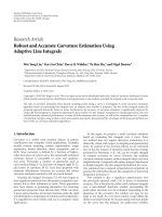
Figure 1: (a) SINR performance in the case of two interferers. (b)
Normalized projection error in the case of two interferers. (c) Di-
rection cosine performance in the case of two interferers.
In the first simulation experiment, we consider the case
when there are two interferers whose received powers are
10 dB stronger than the desired user. Figure 1 shows the sim-
ulation results. It can be observed that the eigenmethod and
the proposed algorithm outperform the TTJ algorithm. The
reason is that the TTJ algorithm belongs to the stochastic gra-
0 100 200 300 400 500
Number of symbol intervals
−25
−20
−15

−10
−5
0
5
10
15
20
Average SNR (dB)
Maximum
Eigen method
Proposed algorithm
TTJ algorithm
SMIT
(a)
0 100 200 300 400 500
Number of symbol intervals
0
0.2
0.4
0.6
0.8
1
Normalized projection er ror
Eigen method
Proposed algorithm
TTJ algorithm
SMIT
(b)
0 100 200 300 400 500
Number of symbol intervals

0
0.2
0.4
0.6
0.8
1
Direction cosine
Eigen method
Proposed algorithm
TTJ algorithm
SMIT
(c)
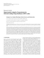
Figure 2: (a) SINR performance in the case of five interferers. (b)
Normalized projection error in the case of five interferers. (c) Di-
rection cosine performance in the case of five interferers.
dient algorithm class and its fixed step size is chosen based on
some tradeoff between tr acking capability and accuracy; too
small a value will bring on slow convergence and too large
a value will lead to overshoot and instability [19]. The eigen
method and SMIT have the best performance. However, their
computational complexity is very high. Compared to these
Jian Yang et al. 7
0 200 400 600 800
Number of symbol intervals
−30
−20
−10
0
10
20

Average SNR (dB)
Maximum
Eigen method
Proposed algorithm
TTJ algorithm
SMIT
(a)
0 200 400 600 800
Number of symbol intervals
0
0.2
0.4
0.6
0.8
1
Normalized projection er ror
Eigen method
Proposed algorithm
TTJ algorithm
SMIT
(b)
0 200 400 600 800
Number of symbol intervals
0
0.2
0.4
0.6
0.8
1
Direction cosine

Eigen method
Proposed algorithm
TTJ algorithm
SMIT
(c)
Figure 3: (a) SINR performance in the dynamical signal environ-
ment. (b) Normalized projection error in the dynamical s ignal envi-
ronment. (c) Direction cosine performance in the dynamical signal
environment.
methods, the complexity of the proposed algorithm has been
greatly reduced, while its performance degrades only slightly.
The simulation results also show that the approximation of
the Hessian matrix and the projection approximation have
little influence on the performance of the proposed algo-
rithm, since its performance approaches that of the eigen
method, which uses neither of these approximation tech-
niques.
In the next simulation experiment, we investigate the per-
formance of the proposed algorithm in a signal environment
with strong interference. We assume that there are two 10 dB,
two 20 dB, and one 30 dB interferers. The simulation results
in Figure 2 show that the performance of the eigen method
and the proposed algorithm hardly changes, whereas the per-
formance of the TTJ algorithm degrades rapidly. This is not
surprising because at each step the TTJ algorithm uses a sin-
gle instantaneous sample to update the weight vector, and
as a result, the estimated weight vector oscillates around the
MSINR combining weight vector. As the number and pow-
ers of the interferers increase, the oscillation becomes more
dramatic and the amplitude increases. Consequently, the av-

eraged performance degrades greatly in this scenario. In con-
trast, the proposed algorithm uses all of the data samples
available up to the time instant n + 1 to estimate the opti-
mal weight vector, and as a result, it performs well in a sig-
nal environment with strong interference. This experiment
also shows that in the case with strong interferers, using the
Hessian matrix approximation and the projection approxi-
mation has only a slight impac t on the performance of the
proposed algorithm.
In the final experiment, we study the tracking capabil-
ity of the proposed algorithm in a dynamic environment. At
the beginning, there are two 10 dB interferers, and at symbol
interval 400, three 20 dB, one 30 dB, and one 40 dB interfer-
ers are added. Figure 3 shows the simulation results. Because
there are few interferers and their powers are not very strong
in the first phase, the TTJ algorithm performs very well. But
in the second phase, too much interference and unregulated
fixed step size cause the performance to degrade greatly. It
can be observed that the eigen method, SMIT, and the pro-
posed algorithm can rapidly adapt to the suddenly changed
signal environment. This is because of using the forgetting
factor in the recursive covariance matrix estimator. The sim-
ulation results also show that in time-varying environment
the influence of the Hessian matrix approximation and the
projection approximation is small.
Therefore, from the above simulation results in various
signal environments, we conclude that the proposed algo-
rithm has rapid convergence, sufficient estimation accuracy,
and good t racking capability. These properties make it very
useful in a practical signal environment, especially when the

interfering power increases due to many practical reasons,
such as too many interferers, incorrect power control, time-
varying channel.
5. CONCLUSIONS
In this paper, we have studied the principal generalized
eigenvector estimation problem. We proposed a new uncon-
strained cost function for the generalized eigendecomposi-
tion problem. Then, based on the proposed cost function,
we have derived a robust adaptive modified Newton algo-
rithm. The convergence of the proposed algorithm has been
8 EURASIP Journal on Advances in Signal Processing
rigorously analyzed. In addition, we applied the proposed al-
gorithm to the adaptive signal reception problem in multi-
carrier DS-CDMA systems, and the numerical simulation re-
sults show that the proposed algorithm has fast convergence
and excellent tracking capability, which are very useful for a
practical communication environment.
APPENDICES
A. PROOF OF THEOREM 1
Proof. Let
∇
R
and ∇
I
be the gradient operators with respect
to the real and imaginary parts of w. According to [19], the
complex gra dient operator is defined as
∇=(1/2)[∇
R
+

j
∇
I
]. After some calculation, we can derive the gradient of
J(w)as
∇J(w) = R
x
w − R
y
w

w
H
R
y
w

−1
. (A.1)
When w
= u
i
, it is easy to show that ∇J(u
i
) = 0. This implies
that any R
x
-orthonormalized generalized eigenvector, u
i
,of

(R
y
, R
x
) is the stationary point of J(w).
Conversely,
∇J(w) = 0means
R
y
w =

w
H
R
y
w

R
x
w. (A.2)
Hence, w is the generalized eigenvector of (R
y
, R
x
), and the
corresponding generalized eigenvalue is (w
H
R
y
w). Premulti-

plying the both sides of (A.2)withw
H
we have
w
H
R
y
w =

w
H
R
y
w

w
H
R
x
w

. (A.3)
Since R
y
is positive definite, w
H
R
y
w > 0forw = 0. There-
fore, we get w

H
R
x
w = 1. This shows that stationary point, w,
of J(w) is the R
x
-orthonormalized generalized eigenvector of
(R
y
, R
x
).
From above analysis, we conclude that w is a stationary
point of J(w)ifandonlyifw is the R
x
-orhtonormalized gen-
eralized eigenvector of (R
y
, R
x
).
Let H
=∇∇
H
J(w) be the M × M Hessian matrix [7]of
J(w) with respect to the vector w. After some calculations,
the Hessian mat rix H is given as
H
= R
x

− R
y

w
H
R
y
w

−1
+

w
H
R
y
w

−2
R
y
ww
H
R
y
.
(A.4)
Since R
x
is positive definite, we have R

x
= VV
H
,where
V is an invertible M
× M matr ix. Let e
i
= V
H
u
i
and C =
V
−1
R
y
(V
−1
)
H
. According to (21)weobtain
Ce
i
= λ
i
e
i
,
e
H

i
e
j
= δ
ij
.
(A.5)
Obviously, λ
i
and e
i
are the eigenvalue and the corresponding
eigenvector of C.
Let e
= V
H
w.Thenweget
H
= V

I −
C
e
H
Ce
+
Cee
H
C


e
H
Ce

2

V
H
= VF(e)V
H
,(A.6)
where
F(e)
= I −
C
e
H
Ce
+
Cee
H
C

e
H
Ce

2
. (A.7)
From the fact that e

H
1
Ce
1
= λ
1
and Ce
1
e
H
1
= λ
2
1
e
1
e
H
1
we
have
F

±
e
1

=
I −
C

λ
1
+ e
1
e
H
1
,
F

± e
1

e
1
= e
1
,
F

±
e
1

e
i
=

1 −
λ

i
λ
1

e
i
,
(A.8)
where i
= 2, , M. Since (1 − λ
i
/λ
1
) > 0, all the eigenvalues
of F(e
1
) are positive. We can conclude that F(e)ispositive
definite at the point e
=±e
1
. Similarly, we can derive
F

e
i

e
1
=


1 −
λ
1
λ
i

e
1
,
F

e
i

e
i
= e
i
,
(A.9)
where i
= 2, , M.Because(1− λ
1
/λ
i
) < 0, F(e
i
) is neither
positive definite nor negative definite. According to (A.6), we
have

H
|
w=±u
i
= VF

e
i

V
H
. (A.10)
It is clear that H is positive definite at the stationary point
w
= u
1
. At any other stationary point u
i
(i = 2, , M), H
is neither positive definite nor negative definite. This means
that w
= u
1
is the unique global minimal point of J(w), and
the other stationary points u
i
(i = 2, , M) are saddle points
of J(w ).
B. PROOF OF THEOREM 3
Proof. The vector w(t) can be expressed as a linear combi-

nation of M generalized eigenvectors u
i
of (R
y
, R
x
), which is
given by
w(t)
=
M

i=1
α
i
(t)u
i
,(B.1)
where α
i
(t)arecomplexcoefficients.
Substituting (B.1) into (38 ) and premultipying by u
H
l
R
x
yield
dα
l
(t)

dt
=

M

i=1
λ
i


α
i
(t)


2

2
+
M

i=1
λ
2
i


α
i
(t)



2

−1
·

2λ
l
α
l
(t)
M

i=1
λ
i


α
i
(t)


2

−
α
l
(t).

(B.2)
Under the assumption u
H
1
R
x
w(0) = 0wecandefineθ
l
=
α
l
(t)/α
1
(t), l = 2, , M. Then we have
dθ
l
dt
=

α
1
(t)
dα
l
(t)
dt
− α
l
(t)
dα

1
(t)
dt

α
−2
1
(t). (B.3)
Jian Yang et al. 9
Substituting (B.2) into (B.3) yields
dθ
l
dt
=−

λ
1
− λ
l

κ(t)θ
l
(t), (B.4)
where
κ(t)
=

2
M


i=1
λ
i


α
i
(t)


2

×

M

i=1
λ
i


α
i
(t)


2

2
+

M

i=1
λ
2
i


α
i
(t)


2

−1
.
(B.5)
Since κ(t) > 0forallt>0, lim
t→∞
θ
l
= 0, l = 2, , M.
It follows that lim
t→∞
α
l
(t) = 0, l = 2, , M,andw(t) =
α
1

(t)u
1
is an asy mptotically stable solution of (38).
Therefore, when t is large enough and l
= 1, (B.2)canbe
simplified as
dα
1
(t)
dt
=
α
1
(t)

1 −


α
1
(t)


2

1+


α
1

(t)


2
. (B.6)
In order to show that lim
t→∞
α
1
(t)=1wedefinez(t) =

α
1
(t)
2
and V[z(t)] = [z(t) − 1]
2
. Their time derivatives
are
˙
z(t)
= α
∗
1
(t)
˙
α
1
(t)+
˙

α
∗
1
(t)α
1
(t)
= 2


α
1
(t)


2
1 −


α
1
(t)


2
1+


α
1
(t)



2
,
˙
V

z(t)

=
2

z(t) − 1

˙
z(t)
=−4

1 −


α
1
(t)


2

2



α
1
(t)


2
1+


α
1
(t)


2
.
(B.7)
According to the theory of Lyapunov stability, V(z)isaLya-
punov function, and z
= 1 is asymptotically stable. More-
over , from (B.6) and lim
t→∞
α
1
(t)=1, we can conclude
lim
t→∞
α
1

(t) = γ,whereγ=1. Hence, w(t)in(38)will
asymptotically converge to the stable solution γu
1
.
ACKNOWLEDGMENT
The authors would like to express their sincerest appreciation
to the anonymous reviewers for their comments and sugges-
tions that sig nificantly improve the quality of this work.
REFERENCES
[1] J. Lu, K. N. Plataniotis, and A. N. Venetsanopoulos, “Face
recognition using LDA-based algorithms,” IEEE Transactions
on Neural Networks, vol. 14, no. 1, pp. 195–200, 2003.
[2] S. Fidler, D. Sko
ˇ
caj, and A. Leonardis, “Combining reconstruc-
tive and discriminative subspace methods for robust classifi-
cation and regression by subsampling,” IEEE Transactions on
Pattern Analysis and Machine Intelligence, vol. 28, no. 3, pp.
337–350, 2006.
[3] T. F. Wong, T. M. Lok, J. S. Lehnert, and M. D. Zoltowski, “A
linear receiver for direct-sequence spread-spectrum multiple-
access systems with antenna arrays and blind adaptation,”
IEEE Transactions on Information Theory,vol.44,no.2,pp.
659–676, 1998.
[4] J. Yang, H. Xi, F. Yang, and Y. Zhao, “Fast adaptive blind beam-
forming algorithm for antenna array in CDMA systems,” IEEE
Transactions on Vehicular Technology, vol. 55, no. 2, pp. 549–
558, 2006.
[5] B. Yang, “Projection approximation subspace tracking,” IEEE
Transactions on Signal Processing, vol. 43, no. 1, pp. 95–107,

1995.
[6] S. Ouyang, P. C. Ching, and T. Lee, “Robust adaptive quasi-
Newton algorithms for eigensubspace estimation,” IEE Pro-
ceedings: Vision, Image and Signal Processing, vol. 150, no. 5,
pp. 321–330, 2003.
[7] A. Hyv
¨
arinen, J. Karhunen, and E. Oja, Independent Compo-
nent Analysis, John Wiley & Sons, New York, NY, USA, 2001.
[8] G. H. Golub and C. F. VanLoan, Matrix Computations,John
Hopkins University Press, Baltimore, Md, USA, 1991.
[9] G. Mathew and V. U. Reddy, “A quasi-Newton adaptive algo-
rithm for generalized symmetric eigenvalue problem,” IEEE
Transactions on Signal Processing, vol. 44, no. 10, pp. 2413–
2422, 1996.
[10]C.Chatterjee,V.P.Roychowdhury,J.Ramos,andM.D.
Zoltowski, “Self-organizing algorithms for generalized eigen-
decomposition,” IEEE Transactions on Neural Networks, vol. 8,
no. 6, pp. 1518–1530, 1997.
[11] D. Xu, J. C. Principe, and H C. Wu, “Generalized eigende-
composition with an on-line local algorithm,” IEEE Signal Pro-
cessing Letters, vol. 5, no. 11, pp. 298–301, 1998.
[12] D. R. Morgan, “Adaptive algorithms for solving generalized
eigenvalue signal enhancement problems,” Signal Processing,
vol. 84, no. 6, pp. 957–968, 2004.
[13] Y. N. Rao, J. C. Principe, and T. F. Wong, “Fast RLS-like al-
gorithm for generalized eigendecomposition and its applica-
tions,” The Journal of VLSI Signal Processing, vol. 37, no. 2-3,
pp. 333–344, 2004.
[14] J. Yang, H. Xi, F. Yang, and Y. Zhao, “RLS-based adaptive al-

gorithms for generalized eigen-decomposition,” IEEE Transac-
tions on Signal Processing, vol. 54, no. 4, pp. 1177–1188, 2006.
[15] T. M. Lok, T. F. Wong, and J. S. Lehnert, “Blind adaptive sig-
nal reception for MC-CDMA systems in Rayleigh fading chan-
nels,” IEEE Transactions on Communications,vol.47,no.3,pp.
464–471, 1999.
[16] S. Kondo and L. B. Milstein, “Performance of multicarrier
DS CDNA systems,” IEEE Transactions on Communications,
vol. 44, no. 2, pp. 238–246, 1996.
[17] J. G. Proakis, Digital Communications, McGraw-Hill, New
York, NY, USA, 1995.
[18] J.Namgoong,T.F.Wong,andJ.S.Lehnert,“Subspacemul-
tiuser detection for multicarrier DS-CDMA,” IEEE Transac-
tions on Communications, vol. 48, no. 11, pp. 1897–1908, 2000.
[19] S. Haykin, Adaptive Filter Theory, Prentice-Hall, Upper Saddle
River, NJ, USA, 2002.
[20] L. Ljung, “Analysis of recursive stochastic algorithms,” IEEE
Transactions on Automatic Control, vol. 22, no. 4, pp. 551–575,
1977.
[21] H. J. Kushner and D. S. Clark, Stochastic Approximation Meth-
ods for Constrained and Unconstrained Systems,Springer,New
York, NY, USA, 1978.
[22] D. R. Morgan, J. Benesty, and M. M. Sondhi, “On the evalu-
ation of estimated impulse responses,” IEEE Signal Processing
Letters, vol. 5, no. 7, pp. 174–176, 1998.
[23] T. M. Lok and T. F. Wong, “Transmitter and receiver opti-
mization in multicarrier CDMA systems,” IEEE Transactions
on Communications, vol. 48, no. 7, pp. 1197–1207, 2000.
10 EURASIP Journal on Advances in Signal Processing
Jian Yang received the B.S., M.S., and Ph.D.

degrees from the University of Science and
Technology of China (USTC), Hefei, China,
in 2001, 2003, and 2005, respectively. He
is currently with the Laboratory of Net-
work Communication System and Control
in USTC. His research area is multime-
dia communication and signal processing,
including adaptive streaming media sys-
tem design and performance optimization,
adaptive load balance, adaptive filtering, antenna array signal pro-
cessing, and frequency estimation.
Feng Yang received the B.S. degree in elec-
trical engineering from Tongji University,
Shanghai, China, in 2001, and the M.S. de-
gree from USTC, Hefei, China, in 2003. He
is currently pursuing the Ph.D. degree. His
current research interests include adaptive
filtering theory, MC-CDMA systems, and
MIMO systems.
Hong-Sheng Xi received the B.S. and M.S.
degrees in applied mathematics from the
University of Science and Technology of
China (USTC), Hefei, China, in 1980 and
1985, respectively. He is currently the Dean
of the Department of Automation at USTC.
He also directs the Laboratory of Network
Communication System and Control. His
research interests include stochastic con-
trol systems, discrete-event dynamic sys-
tems, network performance analysis and optimization, and wireless

communications.
Wei Gu o received his B.S. degree and Ph.D.
degree in China University of Science and
Technology and Chinese Academy of Sci-
ences in 1983 and 1992, respectively. He
worked in Communication Research Lab-
oratory, Japan, and Hong Kong Univer-
sity of Science and Technology, in 1994-
1995 and 1998, respectively. Professor Wei is
the Member of the Communication Expert
Group, State High Technology Project (863
Project), and the core Member of the Technical Group, China 3G
Mobile Communication System Project. His current research inter-
ests are the concept and key technology for the 4G Mobile Commu-
nication system.
Yanmin Sheng received the B.S. degree in
automation from University of Science and
Technology of China, Hefei, China, in 2002,
the Ph.D. degree in control science and en-
gineering from University of Science and
Technology of China, Hefei, China, in 2007.
He has worked in areas of wireless commu-
nication, adaptive theory, and application,
and statistical theory. His current research
interests include particle filter application in
communication, OFDM, and MIMO.