Báo cáo hóa học: " Research Article Edge Adaptive Color Demosaicking Based on the Spatial Correlation of the Bayer Color Difference" pptx

Hindawi Publishing Corporation
EURASIP Journal on Image and Video Processing
Volume 2010, Article ID 874364, 14 pages
doi:10.1155/2010/874364
Research Article
Edge Adaptive Color Demosaicking Based on
the Spatial Correlation of the Bayer Color Difference
Hyun Mook Oh, Chang Won Kim, Young Seok Han, and Moon Gi Kang
TMS Institute of Information Technology, Yonsei University, 134 Shinchon-Dong, Seodaemun-Gu,
Seoul 120-749, Republic of Korea
Correspondence should be addressed to Moon Gi Kang,
Received 10 April 2010; Revised 25 June 2010; Accepted 24 September 2010
Academic Editor: Lei Zhang
Copyright © 2010 Hyun Mook Oh et al. This is an open access article distributed under the Creative Commons Attribution
License, which permits unrestricted use, distribution, and reproduction in any medium, provided the original work is properly
cited.
An edge adaptive color demosaicking algorithm that classifies the region types and estimates the edge direction on the Bayer color
filter array (CFA) samples is proposed. In the proposed method, the optimal edge direction is estimated based on the spatial
correlation on the Bayer color difference plane, which adopts the local directional correlation of an edge region of the Bayer CFA
samples. To improve the image quality with the consistent edge direction, we classify the region of an image into three different
types, such as edge, edge pattern, and flat regions. Based on the region types, the proposed method estimates the edge direction
adaptive to the regions. As a result, the proposed method reconstructs clear edges with reduced visual distortions in the edge and
the edge pattern regions. Experimental results show that the proposed method outperforms conventional e dge-directed methods
on objective and subjective criteria.
1. Introduction
Single chip CCD or CMOS imaging sensors are widely
used in digital still cameras (DSCs) to reduce the cost and
size of the equipments. Such imaging sensors obtain pixel
information through a color filter array (CFA), such as
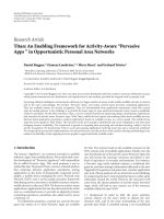
Bayer CFA [1]. When the Bayer CFA is used in front of
the image sensor, one of the three spectral components

(red, green, or blue) is passed at each pixel location as
shown in Figure 1(a). In order to obtain the full color image,
the missing color components should be estimated from
the existing pixel information. This reconstruction process
is called color demosaicking or color interpolation [2–25].
Generally, the correlation between color channels is utilized
by assuming the smoothness color ratio [ 3, 4] or smoothness
color difference [5–7].Thesemethodsproducesatisfactory
results in a homogeneous reg ion, while visible artifacts (such
as zippers, Moir
´
eeffects, and blurring artifacts) are shown in
edge regions.
In order to reduce interpolation errors in these regions,
various approaches have been applied to color demosaicking.
In [8–12], various edge indicators were used to prevent
interpolation across edges. Gunturk et al. decomposed color
channels into frequency subbands and updated the high-
frequency subbands by applying a projection onto convex-
sets (POCS) technique [13]. Zhang and Wu modeled color
artifacts as noise factors and removed them by fusing the
directional linear minimum mean squares error (LMMSE)
estimates [14]. Alleysson et al. proposed frequency selective
filters which adopt localization of the luminance and chromi-
nance frequency components of a mosaicked image [15]. All
of these approaches show highly improved results on the edge
regions. However, the interpolation error and smooth edges
in edge patterns or edge junctions are challenging issues in
demosaicking methods.
As an approach to reconstruct the sharp edge, edge

directed color demosaicking algorithms were proposed
which aimed to find the optimal edge direction at each pixel
location [16–25]. Since the inter polation is performed along
the estimated edge direction, the edge direction estimation
techniques play a main roll in these methods. In some meth-
ods [20–22], the edge directions of missing pixels are indi-
rectly estimated in aid of the additional information from the
horizontally and vertically prereconstructed images. Wu and
2 EURASIP Journal on Image and Video Processing
RR
RR
RR
RR
B
B
B
B
BB
BB
B
G
G
G
G
GG
GG
G
G
GG
GG

G
Down-
sampling
G
00
R
01
B
10
G
11
(a) (b)
Figure 1: (a) The Bayer CFA pattern and (b) the down sampled low
resolution images.
Zhang found the edge direction based on the Fisher’s linear
discriminant so that the chance of the misclassification of
each pixel is minimized [20]. Hirakawa and Parks proposed a
homogeneity map-based estimation process, which a dopted
the luminance and chrominance similarities between the
pixels on an edge [21]. Menon et al. proposed the direction
estimation scheme using the smoothness color differences on
the edges, where the color difference was obtained based on
the directionally filtered green images [22]. In these methods,
the sharp edges are effec tively restored with the temporally
interpolated images. However, the insufficient consideration
for the competitive regions results in outstanding artifacts
due to the inconsistent directional edge interpolation.
Recently, some methods that directly deal with the CFA
problems such as CFA sampling [23–25], CFA noise [26]or
both of the problems [27] were proposed. These methods

studied the characteristics of the CFA samples and recon-
structed the image without the CFA error propagation and
the inefficient computations due to the preinterpolation pro-
cess. Focusing on the demosaicking directly on the CFA sam-
ples, Chung and Chan studied the color difference variance
of the pixels located along the horizontal or the vertical axis
of CFA samples [23]. Tsai and Song introduced the concept
of the spectral-spatial correlation (SSC) which represented
the direct difference between Bayer CFA color samples [24].
Based on the SSC, they proposed heterogeneity-projection
technique that used the smoothness derivatives of the Bayer
sample differences on the horizontal or vertical edges. Based
on the Tsai and Song’s method, Chung et al. proposed
modified heterogeneity-projection method that adaptively
changed the mask size of the derivative [25].
As shown in [24, 25], difference of the Bayer samples
provides key to directly estimate the edge direction on the
Bayer pattern. In the conventional SSC-based methods, the
smoothness of the Bayer color difference along an edge is
examined, and the derivative of the differences along the hor-
izontal or vertical axis is adopted as a criterion for edge direc-
tion estimation. However, in the complicated edge region,
such as edge patterns or edge junctions, the edge direction
is usually indistinguishable since derivatives along the line
are very close to the horizontal and vertical directions. To
carry out more accurate interpolation on these regions,
region adaptive interpolation scheme which estimates the
edge direction adaptive to the region types with the given
directional correlation on Bayer color difference is required.
In this paper, a demosaicking method that estimates the

edge direction directly on the Bayer CFA samples is proposed
based on the spatial correlation of the Bayer color difference.
To estimate the edge direction with accuracy, we investigate
the consistency of the Bayer color difference within a local
region. We focus on the local similarity of the Bayer color
difference plane not only along the directional axis but
also beside the axis within the local region. Since the edge
directions of the pixels on and around the edge contribute
to the estimation simultaneously, the correlation adopted in
the proposed method is a stable and effective basis to estimate
the edge direction in the complicated edge regions. Based on
the spatial correlation on the Bayer color difference plane,
we propose an edge adaptive demosaicking method that
classifies an image into edge, edge pattern, and flat regi ons,
and that estimates the edge direction according to the region
type. From the result of the estimated edge direction, the
proposed method interpolates the missing pixel values along
the edge direction.
The rest of the paper is organized as follows. Using
the difference plane of the down sampled CFA images, the
spatial correlation on the Bayer color difference plane is
examined in Section 2. Based on the examined correlation
between the CFA sample di
fferences, the proposed edge
adaptive demosaicking method is described with the criteria
for the edge direction detection and the region classification
in Section 3. Also, the interpolation scheme along the
estimated edge direction is depicted, which aims to restore
the missing pixels with reduced artifacts. Section 4 presents
comparisons between the proposed and conventional edge

directed methods in terms of the quantitative and qualitative
criteria. Finally, the paper is concluded with Section 5.
2. Spatial Correlation on
theBayerColorDifferencePlane
In the proposed method, the region type and the edge
direction are determined directly on the Bayer CFA samples
based on the correlation of the Bayer color difference. For the
efficient criteria for these main parts of the proposed demo-
saicking method, the Bayer color difference is reexamined on
the down sampled low-resolution (LR) Bayer image plane
so that the direction-oriented consistency of the Bayer color
differences is emphasized within the local region of an edge.
The Bayer color difference is a strong relation between
the CFA samples on a horizontal or vertical line [24],
followed as
D
h( j,j+1)
rg
= R

i, j

−
G

i, j +1

=

R


i, j

−

G

i, j


−

G

i, j +1

−

G

i, j


,
D
v(i,i+1)
rg
= R

i, j


− G

i +1,j

=

R

i, j

−

G

i, j


−

G

i +1,j

−

G

i, j



,
(1)
EURASIP Journal on Image and Video Processing 3
h
0
(i)
h
1
(i)
h
0
( j)
h
0
( j)
h
1
( j)
h
1
( j)
G
LL
00
= G
00
G
00
G

LH
00
=

G
ver
00
G
HL
00
=

G
hor
00
G
HH
00
=

G
n
00
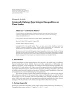
Figure 2: Undecimated 2D wavelet transform with filter banks and
spectral components of G
00
.
where the R(i, j), and G(i, j) are Bayer CFA samples of
red and green channels in (i, j) pixel location, respectively,


G(i, j) is a missing sample of green channel, and D
h( j,j+1)
rg
and D
v(i,i+1)
rg
are the Bayer color difference on the horizontal
and vertical directional lines, respectively. The Bayer color
difference is assumed piecewise constant along an edge
since it inher its the characteristics of spectral and spatial
correlations [24].
From the relation between the CFA samples on a line,
we expand the CFA sample relation into the Bayer color
difference plane which is defined by the difference of Bayer
LR images. When we consider the down sampling of the
Bayer CFA image as shown in Figure 1, each of the LR image
is obtained according to the sampling position of each color
channel, given as
C
xy

i, j

= CFA

2i + x,2j + y

,
(2)
where CFA(i, j) represent the Bayer CFA samples at pixel

index (i, j) and the LR image channel C is green, red, blue,
and green channels according to the sampling index
{(x, y) |
(0, 0), (0, 1), (1, 0), (1, 1)}, respectively. Therefore, we obtain
four LR images
{G
00
, R
01
, B
10
, G
11
}, and each of them has full
spatial resolution in LR grid as shown in Figure 1(b). Using
the defined LR images, the Bayer color difference plane is
defined as the difference between the LR images,
D
C1
xy
C2
zw
= C1
xy
− C2
zw
,
(3)
where D
C1

xy
C2
zw
is the Bayer color difference plane given the
different Bayer LR images, C1
xy
/
= C2
zw
. Note that, the cor-
relation between the sampling positions are simultaneously
considered with the inter channel correlation in (3).
To describe the local property of D
C1
xy
C2
zw
, we consider
the directional components of LR images. When we use
the undecimated wavelet transform, a LR image can be
decomposed into low-frequency, horizontal, vertical direc-
tional and the residual high frequency components [13]. As
shown in Figure 2 , the two-staged directional low-pass and
the high-pass filters, h
0
(i)andh
1
( j), respectively, make the
low-pass and directionally high-pass filtered images. Given
the directional forward filter banks, a Bayer LR image C

xy
is
represented as the sum of four frequency components, such
as,
C
xy
= C
LL
xy
+ C
LH
xy
+ C
HL
xy
+ C
HH
xy
≈ C
xy
+

C
ver
xy
+

C
hor
xy

,
(4)
where the upper letters LL, LH, HL, HH represent the low fre-
quency, vertical and horizontal directional high frequencies,
and the residual components of C
xy
, respectively, and they
are described as
C
xy
,

C
ver
xy
,and

C
hor
xy
.In(4), it is assumed that
the most of the high-frequencies of an image is concentrated
on the vertical and horizontal directional components, so
that the residual parts are not considered in the following
discussion. Also, the directional high frequency components
are assumed to be exclusively separated in the horizontal
and vertical directions, since an image has strong directional
correlation along the sharp edges. Therefore,

C

hor
xy
(or

C
ver
xy
)is
approximately zero in the vertical (or horizontal) sharp edge
region in (4). Based on these assumptions, the Bayer color
difference plane in (3) is reorganized as follows,
D
C1
xy
C2
zw
= C1
xy
− C2
zw
≈ K +
(
1 − δ
(
x − z
))


C1
hor

xy
−

C1
hor
zw

+

1 − δ

y − w



C1
ver
xy
−

C1
ver
zw

,
(5)
where K
= C1
zw
− C2

zw
represents the spectral correlation
between the Bayer LR images [7], and δ(a
− b) indicates
the LR image shift direction where the value 1 for a
=
b represents no shift, and 0 for a
/
= b represents the shift
toward the direction. Note that, the horizontal (or verti-
cal) directional frequency components are paired with the
vertical (or horizontal) directional shifting indicator. The
cross-directional pair of shift indicator and the directional
frequencies shows the relation between the global LR image
shifting direction and the local edge direction: the Bayer
color difference is highly correlated in a local region when the
global shift and the local edge directions are corresponded to
each other. We call it as the spatial correlation of the Bayer
color difference.
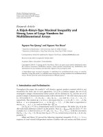
In Figure 3, a vertical edge region is shown as an example
of the relation between the global and the local directions.
When the vertical region in the 6
× 6 local region of Baye r
pattern in Figure 3(a) is down sampled, the corresponding
LR images in Figure 3(b) show different edge locations
according to the sampling location. When the global shift
direction coincides with the vertical local direction, Bayer
LR images show similar edge location. Otherwise, the edges
in each image are dislocated. From (5), the Bayer color
difference planes that is obtained by R

01
and horizontally and
vertically shifted images G
00
and G
11
, respectively, are given
as follows:
D
G
00
R
01
= K +

C1
ver
xy
−

C1
ver
zw
D
G
11
R
01
= K.
(6)

4 EURASIP Journal on Image and Video Processing
Down-
sampling
Bayer color
difference plane
R
R
R
GG
G
G
G
G
G
R
R
R
G
G
G
R
R
R
R
R
R
R
R
R
R

R
R
G
G
G
G
G
BB
B
B
B
B
G
G
G
B
B
B
B
B
B
B
B
B
B
B
B
G
G
G

G
G
G
G
G
G
G
G
G
G
G
G
G
G
G
B
10
Bayer pattern
(vertical edge region)
R
01
G
11
(G-R)
D
h
D
h
D
h

D
h
D
h
D
h
D
h
D
h
D
h
D
v
D
v
D
v
D
v
D
v
D
v
D
v
D
v
D
v

D
h
= G
00
− R
01
G
00
D
v
= G
11
− R
01
(a) (b)
(c)
Figure 3: Vertical edge region of (a) Bayer CFA samples, (b) Bayer LR images, and (c) the Bayer color difference planes.
In (6), the difference of vertical high frequency components
are remained in the difference of horizontally shifted LR
images, while they are disappeared in the difference of
vertically shifted LR images. In the real images, the spatial
correlation on the Bayer color difference plane can be
shown as depicted in Figure 4. In the strong vertical edge
region in Figure 4(a), the difference plane obtained from
the vertically shifted LR images is smooth planes, while
the difference obtained from the horizontally shifted images
shows overstated details. In the edge pattern region in
Figure 4(b), the aliasing effect of the LR images makes
pattern in the difference plane from the horizontally shifted
images. However, the aliasing effects are disappeared in the

difference plane of the opposite case. From these examples,
the strong connection of the global shift direction and the
local edge direction is described by the spatial correlation of
Bayer color difference. In the following section, we describe
the detailed method to use the spatial correlation of the Bayer
color difference in the edge direction estimation and the
region classification.
3. Proposed Edge Directed Color Demosaicking
Algorithm Using Region Classifier
In the proposed edge adaptive demosaicking method, the
edge directions are optimally estimated according to the
region type. Based on the spatial correlation of the Bayer
color difference, the proposed method classifies an image
into three regions, such as edge, edge pattern, and flat
regions. In each of the regions, we classify the edge direction
type (EDT) as the horizontal (Hor) or vertical (Ver) direc-
tion. When the direction is not obviously determined, we
decide the direction as nondirectional (Non). Therefore, the
final types of the edge direction are EDT
={Hor, Ver, Non}.
In the proposed edge direction estimation, the diagonal
directional edge is considered as the combination of the
horizontal and vertical directional edges. According to the
determined edge direction, the missing pixels are interpo-
lated with weighting functions. Following the edge types
and the edge directions, we present the way to classify the
region and to estimate the edge direction based on the spatial
correlation on the Bayer color difference plane. To utilize
R
01

R
01
G
00
G
11
G
00
G
11
D
G
00
R
01
= G
00
− R
01
=
=
=
=
D
G
11
R
01
= G
11

− R
01
D
G
00
R
01
= G
00
− R
01
D
G
11
R
01
= G
11
− R
01
−
−
(a)
(b)
Figure 4: Examples of the Bayer color difference planes of R
01
and
G
00
and R

01
and G
11
(a) edge and flat regions (b) vertical edge
pattern region.
the correlation, we describe the details of the interpolation
process as the restoration of missing channels of LR images.
Given the obtained LR images BAYER
={G
00
, R
01
, B
10
, G
11
}
in Figure 1(b), the missing channels of each LR color images
are
{G
01
, G
10
, R
00
, R
10
, R
11
, B

00
, B
01
, B
11
}. By considering the
sampling rate of the green channel, the proposed method
first interpolates the missing green channels, than the red and
blue channels are interpolated by using the fully interpolated
green channel images. This is helpful to improve the red
and blue channel interpolation quality, since the green
channel has more edge information than the red and blue
channels. Since the Bayer LR images are shifted to each other,
they are interpolated in the same way for each channel.
EURASIP Journal on Image and Video Processing 5
Once all of the missing channels are reconstructed at each
sampling position, the full-color LR images are upsampled
and they are registered according to the original position in
the HR grid. The overall process of the proposed adaptive
demosaicking method is depicted in Figure 6, where the
process is composed of estimating Bayer color difference
plane, the region classification, the edge direction estimation,
and the directional interpolation for each green and red/blue
channel interpolation. In the following subsections, the
way of interpolating the missing pixels in G
01
and R
00
are
described as a representative of green and red(blue) channel

interpolations.
3.1. Green Channel Interpolation
3.1.1. Region Classification: Sharp Edges. In the proposed
demosaicking method, the modified notation for the sam-
pling index is used to emphasize the relation between the
global shift direction and local edge direction in LR images.
When we consider the interpolation of the missing green
channel of R
01
position, we set the red pixel position as the
center position, that is,
R
c

i, j

=
CFA

2i,2j +1

=
R
01

i, j

.
(7)
According to the center position, the four neighborhood

positions are defined as
G
n

i, j

=
CFA

2i − 1, 2j +1

=
G
11

i − 1, j

,
G
s

i, j

= CFA

2i +1,2j +1

= G
11


i, j

,
G
e

i, j

=
CFA

2i,2j +2

=
G
00

i, j +1

,
G
w

i, j

=
CFA

2i,2j


=
G
00

i, j

,
(8)
where
{n, s, e, w} represents the position of the pixels in the
LR images in the north, south, east, and west from the center
position. Note that the notation inherits the relative pixel
position in Bayer CFA samples from the center pixel position.
Using the modified notation, the Bayer color difference
in (3)isdefinedas
D
G
p
R
c

i, j

=
G
p

i, j

−

R
c

i, j

,
(9)
where p
={n, s, e, w}. From the spatial correlation on the
Bayer color difference plane in (5), D
G
p
R
c
is highly correlated
in the local region when the shifting direction coincides
with the local edge direction. As an estimator for the spatial
correlation, the local variations of the difference is estimated,
such as
υ
p

i, j

=

(
k,l
)
∈N




D
G
p
R
c

i + k, j + l

−
D
G
p
R
c

i, j




, (10)
where N
={(k, l) |−1 ≤ k, l ≤ 1, (k, l)
/
= (0, 0)}.In
Figure 5, the window mask on the Bayer pattern and the
corresponding Bayer color difference planes are described.

When the local variations of each position are determined,
D
GwRc
(= G
w
− R
c
)
D
GnRc
(= G
n
− R
c
)
D
GeRc
(= G
e
− R
c
)
D
GsRc
(= G
s
− R
c
)
G

G
G
G
G
G
G
G
G
G
G
G
G
G
G
G
G
G
G
G
G
G
G
G
R
R
R
R
R
R
R

R
R
B
B
B
B
B
B
B
B
B
B
B
B
B
B
B
B
Figure 5: A 7 × 7 window of Bayer CFA pattern and its four
neighboring Bayer color difference planes for local variation
criterion.
the maximum and the minimum variations of horizontal
shifting direction are defined as:
υ
max
hor

i, j

=

MAX

υ
w

i, j

, υ
e

i, j

,
υ
min
hor

i, j

=
MIN

υ
w

i, j

, υ
e


i, j

.
(11)
Also, υ
max
ver
(i, j)andυ
min
ver
(i, j) are determined as the same
way in (11) by changing
{υ
w
, υ
e
} to {υ
s
, υ
n
}.Theedge
direction is clearly determined owing to the group with
smaller variations, since the maximum of local variations
along the edge direction is smaller than the minimum of local
variations across the edge direction in the strong edge region.
In addition, the spatial similarity between the green
channels is estimated for the restrict decision of the edge
direction. Defining the difference plane of green channel,
D
G

p
G
q

i, j

=
G
p

i, j

−
G
q

i, j

,
(12)
where
{(p, q) | (e, w), (n, s)} is a pair of the horizontally or
vertically located LR image positions. By applying the dis-
cussions in (5), the spatial correlation of D
G
p
G
q
is estimated
by the local similarity for the horizontal and the vertical

directions, such as,
ρ
hor

i, j

=
1

k=−1
1

l=−1


D
G
w
G
e

i + k, j + l



,
ρ
ver

i, j


=
1

k=−1
1

l=−1


D
G
n
G
s

i + k, j + l



,
(13)
where ρ
hor
(i, j)andρ
ver
(i, j) represent the local average of
the differences between the horizontally and vertically shifted
green images, respectively. The local similarity becomes small
6 EURASIP Journal on Image and Video Processing

EDT = { Ver, Hor, non}
Edge adaptive demosaicking
Bayer color
difference
plane
G channel interpolation
Region
classification
Edge
direction
estimation
directional
interpolation
Edge region
Edge-pattern region
Flat region
Bayer color
difference
plane
R/B channel interpolation
Region
classification
Edge
direction
estimation
Bayer CFA
samples
Full color
image
Spatial correlation

Directional
interpolation
Figure 6: Flowchart of the proposed edge adaptive color demosaicking algorithm.
when the global shift and the local edge directions are
coincided.
With the measured local variation and local similarity
criteria, the EDT of each pixel is determined by,
Classification 1. Sharp edge region
EDT
=
⎧
⎪
⎪
⎪
⎪
⎪
⎪
⎪
⎪
⎪
⎪
⎪
⎪
⎪
⎪
⎪
⎨
⎪
⎪
⎪

⎪
⎪
⎪
⎪
⎪
⎪
⎪
⎪
⎪
⎪
⎪
⎪
⎩
Hor
if υ
max
hor
<υ
min
ver
and ρ
hor
<ρ
ver
,
Ver
if υ
min
hor
>υ

max
ver
and ρ
hor
>ρ
ver
,

nonsharp edge region

,
otherwise,
(14)
where Hor and Ver represents the sharp edges along hori-
zontal or vertical directions, respectively. When the direction
is not determined, the region is considered as a nonsharp
edge region and these regions are investigated again in the
following region classification step: Classification 2.
3.1.2. Region Classification: Edge Patterns. The regions of
which edge t ypes are not determined in (14) belong to the
flat or the edge pattern region. The edge pattern region
represents the region in the HR image that contains high-
frequency components above the Nyquist rate of the Bayer
CFA sampling. When the image is down sampled, the high
frequency components that exceed the sampling rate are
contaminated due to the aliasing effect. Therefore, the edge
pattern region appears as locally flat in the LR image as
shown in Figure 4(b). In this section, we derive the detection
rule for the edge pattern region (pseudoflat region in the LR
grid) and estimate the edge direction of the edge pattern.

To distinguish the pseudoflat region from the flat region,
we use the characteristics of aliasing effect in the LR images.
As shown in Figure 4(b), the fence region of G
00
and G
11
are
flat for each images. This phenomenon is caused by the CFA
sampling above the Nyquist rate in these regions and the high
frequencies in HR image is blended into the low frequency
by the down sampling. However, they are not the same flat
when we compare the intensity of them at the same pixel
location since the frequency blending cannot contaminate
the intensity offset between the adjacent edges. Therefore,
we use two criteria to classify the pseudoflat region from the
normal flat region: the intensity offset and the smoothness
restriction. The intensity offset is estimated by
μ

i, j

=





G
n


i, j

+ G
s

i, j

2
−
G
e

i, j

+ G
w

i, j

2





,
(15)
where μ(i, j) is the difference between averages of the
horizontally and vertically located LR images, and
G

p
(i, j)
represents the low frequency of G
p
at (i, j) pixel location.
In addition to intensity offset, we restrict the condition
with the pixel smoothness in respective LR images. Since
we deal with the flat (and also the pseudoflat) region, the
local variation values, which mean the fluctuation on each
of the difference images, should be similar to each other. The
similarity between the local var iation values is estimated by
the standard deviation of the local variations, given by:
σ
υ

i, j

=




1
4

p

υ
p


i, j

− υ

i, j


2
,
(16)
where σ
υ
(i, j)isavariationofυ
p
(i, j)andυ(i, j) is the average
of local variations.
With the intensity offset and the restrictive condition, the
pseudoflat region (edge pattern region) is classified from the
nonsharp edge region, such as
EURASIP Journal on Image and Video Processing 7
Classification 2. Edge pattern or Flat region
EDT
=
⎧
⎨
⎩

edge pattern

if μ>th1, σ

v
<th2,
Non otherwise,
(17)
where edge pattern and Non represent that the region is
determined as the edge pattern region and a flat region in
this classification, respectively, and th1andth2 are thresholds
that control the accuracy of the classification. If μ is larger
(and σ
υ
is smaller) than the threshold, the pixel at (i, j)
is considered as being in the edge pattern region and the
direction of the edge pattern is determined by the following
criteria.
For pixels classified into the edge pattern region, the
pattern edge direction is estimated using the modified local
variation values in (10) with the extended range N
={(k, l) |
−
2 ≤ k, l ≤ 2, (k, l)
/
= (0, 0)}. The edge direction of the edge
pattern region is estimated as
EDT
=
⎧
⎪
⎪
⎪
⎪

⎨
⎪
⎪
⎪
⎪
⎩
Hor if υ
max
hor
<υ
min
ver
Ver if υ
min
hor
>υ
max
ver
Non otherwise,
(18)
where Hor and Ver represent that the edge pattern is
horizontally or vertically directed, respectively, and Non
represents the region of which the edge direction is not
clearly determined. Once the edge type of the edge pattern
region is determined, the statistics of neighboring edge
directions, such as the horizontal or vertical direction, are
compared within a neighborhood. Following the majority of
the directions, the consistency of the edge directions in the
region is improved.
3.1.3. Edge D irected Interp olation. After the edge types of

all pixels are categor ized with the classified region types,
edge directed interpolation is performed. If the edge types
are clearly determined as Hor or Ver, the missing pixels are
interpolated toward the direction. When the edge direction
is determined as Non, it is considered as the flat region or the
region where the edge direction is not defined. In this case,
the missing pixels are interpolated by the weighted average of
neighboring pixels. Therefore, the missing green channel LR
image is interpolated according to the edge types, such as,
G
01
=
⎧
⎪
⎪
⎪
⎪
⎪
⎪
⎪
⎪
⎪
⎪
⎪
⎪
⎨
⎪
⎪
⎪
⎪

⎪
⎪
⎪
⎪
⎪
⎪
⎪
⎪
⎩
ω
e
K
R
e
+ ω
w
K
R
w
ω
e
+ ω
w
+ R
c
if EDT=Hor,
ω
n
K
R

n
+ ω
s
K
R
s
ω
n
+ ω
s
+ R
c
if EDT=Ve r,

ω
n
K
R
n
+ω
s
K
R
s
+ω
e
K
R
e
+ω

w
K
R
w

(
ω
n
+ω
s
+ω
e
+ω
w
)
+R
c
if EDT=Non,
(19)
where ω
p
represent a weight function, and K
R
p
is a color
difference domain value obtained from four green LR image
locations. The weighting function used in the interpolation
process is a reciprocal of gradient magnitude values [10]:
ω
p


i, j

=
1
1+Δ
c
+ Δ
d1
+ Δ
d2
,
(20)
where Δ
c
, Δ
d1
and Δ
d2
represent the gradients of the pixels
in the center image, in the LR images that are shifted
corresponding to the considering direction p, and in the
other LR images, respectively. For example, the weighting
function in the north direction ω
n
(i, j) is calculated from
Δ
c
=|R
c

(i−1, j)−R
c
(i, j)|, Δ
d1
=|G
n
(i−1, j)−G
n
(i, j)|+
|G
s
(i − 1, j) − G
s
(i, j)|,andΔ
d2
=|G
e
(i − 1, j) − G
e
(i, j)| +
|G
w
(i − 1, j) − G
w
(i, j)|.TheK
R
p
values of each LR image are
obtained as followed by using the definition of the difference
between the red and green channels [7]:

K
R
p

i, j

=
G
p

i, j

−
R
c

i, j

+ R
c

i + a, j + b

2
,
(21)
where
{(a, b) | (−1, 0), (1, 0), (0, −1), (0, 1)} is for {p |
n, s, e, w},respectively.
3.2. Red and Blue Channel Interpolation. Similar to the

green plane interpolation, the missing red and blue channel
LR images are interpolated along the edge direction by
the region classification and the edge direction estimation.
The fully interpolated green channels which have much
information on edges are utilized to improve interpolation
accuracy of the red and blue channels. To compensate
insufficient LR images, the diagonally shifted LR images of
{R
01
, B
10
} are estimated using linear interpolation on the
color difference domain [7]. In this section, the missing red
and blue channels
{R
00
, R
11
, B
00
, B
11
} are found in aid of
the sampled images
{G
00
, G
11
, R
01

, B
10
} and the interpolated
images
{G
01
, G
10
, R
10
, B
01
}.
To interpolate the red LR image in (0, 0) sampling
position, G
00
is used as the center image, thatis, G
c
,and
the four neighboring red and green images at each s ide are
used. The red and green images at each sampling position
are defined as R
p
and G
p
where {p | n, s, e, w},respectively,
and R
p
for each position is defined as follows:
R

n

i, j

=
R
10

i − 1, j

,
R
s

i, j

= R
10

i, j

,
R
e

i, j

=
CFA


2i,2j +1

=
R
01

i, j

,
R
w

i, j

= CFA

2i,2j − 1

= R
01

i, j − 1

.
(22)
8 EURASIP Journal on Image and Video Processing
1
2
3
4

5
6
7
8
9
10
11
12
13
14
15
16
17
18
19
20
21 22
23
24
(a)
1
2
(b)
Figure 7: (a) Kodak PhotoCD image set and (b) Bayer raw data.
Considering the four neighboring red and green images
of G
c
, the local variation and local similarity criter ia are
estimated as the same way in (10)and(13) by using the newly
defined D

G
c
R
p
(i, j). When the edge direction is estimated by
(14)and(17) with the process of region classification, R
00
is
directionally interpolated, given as:
R
00
=
⎧
⎪
⎪
⎪
⎪
⎪
⎪
⎪
⎪
⎪
⎪
⎨
⎪
⎪
⎪
⎪
⎪
⎪

⎪
⎪
⎪
⎪
⎩
G
c
−
ω
e
K
R
e
+ ω
w
K
R
w
ω
e
+ ω
w
if EDT=Hor,
G
c
−
ω
n
K
R

n
+ ω
s
K
R
s
ω
n
+ ω
s
if EDT=Ve r,
G
c
−

ω
n
K
R
n
+ω
s
K
R
s
+ω
e
K
R
e

+ω
w
K
R
w

(
ω
n
+ω
s
+ω
e
+ω
w
)
if EDT
=Non,
(23)
where K
R
p
(i, j) = G
p
(i, j) − R
p
(i, j). The weight function is
computed as the same way in (20), but the gradient values
are calculated in the green LR images.
4. Experimental Results

To study performance experimentally, the proposed and
other existing algorithms were tested with Kodak PhothCD
image set and Bayer CFA raw data shown in Figure 7.For
comparison, three groups of conventional methods were
implemented: nonedge directed (nonED) methods proposed
by Pei and Tam [7], by Gunturk et al. [13], and by Zhang
and Wu [14], the indirect edge directed (indirect ED)
methods such as primary-consistency soft-decision (PCSD)
method [20], the homogeneity-directed method [21], and
the a posteriori decision method [22], and the direct edge
directed (direct ED) methods such as the variance of color
differences method [23], and the adaptive heterogeneity-
projection method [25]. They were implemented following
the parameters given in each paper or using the provided
source code [14]. Also, we implemented each of the methods
without the refining step [21–23, 25] so that the perfor-
mances of the methods were compared fairly.
The peak signal-to-noise ratio (PSNR) and the nor-
malized color difference (NCD) were used for quantita-
tive measurement. The PSNR is defined in decibels as
PSNR
= 10 log
10
(255
2
/MSE), where MSE represents the
mean squared error between the original and the resultant
images. The NCD is an objective measurement of the
perceptual errors between the original and the demosaicked
color images [11]. This value is computed by using the

ratio of the perceptual color errors to the magnitude of
the pixel vector of the original image in the CIE Lab color
space. A smaller NCD value represents that a given image is
interpolated with a reduced color artifac t . In Tables 1 and 2,
PSNR and NCD values of each algorithm were compared.
Among the conventional methods, nonED methods, such
as DLLMMSE [14] and POCS [2], show high performance
in terms of the numerical values. Also, the recent edge
directed techniques [21–23, 25] show high PSNR and NCD
performance among the conventional edge directed tech-
niques, especially in the images with fine texture patterns,
such as Kodak5,6,8,15,and19. The proposed method
outperforms the conventional edge directed methods in the
majority of the images including those challenging images
with 0.345–2.191 dB and 0 .003–0.203 improvements of the
averaged PSNR and NCD values, respectively.
EURASIP Journal on Image and Video Processing 9
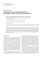
(a) (b) (c) (d) (e)
(f) (g) (h) (i) (j)
Figure 8: The partially magnified images of Kodak 19 from (a) the original image, and from the results of (b) Pei [7], (c) the POCS [13](d)
the directional LMMSE [14], (e) the PCSD [20], (f) the homogeneity-directed [21], (g) a posteriori decision [22], (h) the variance of color
differences [23], (i) the adaptive heterogeneity-projection [25], and (j) the proposed method.
To show the performance of each methods in edge
patterns and edge junctions, the resulting images are shown
in Figures 8–11 that contain fine textures of Kodak 19,
15 and real images, respectively. At first, the competitive
regions of Kodak 19 are show n in Figure 8.Ineachof
the image crop, the vertically directed line edge pattern
of the fence and the edge junctions of the window are
depicted. In spite of the high PSNR performance, POCS

method shows the Moir
´
e pattern and the zipper ar tifacts
in Figure 8(c). In Zhang’s method and the edge directed
methods in Figures 8(d)–8(i), the fence regions are highly
improved with reduced errors. However, visible artifacts were
remained on the vertical edges of the high frequency region
or boundaries between the fence and the grass. Moreover,
the zippers and disconnection were shown in the edge
junctions in the upper image crop in Figures 8(b)–8(i).In
Figure 8(j), the resultant image of the proposed algorithm
shows better results in terms of the clear edges and the
reduced visible artifacts. The resultants of the methods in the
textures with diagonal patterns or diagonal lines are shown
in Figure 9. While the artifacts were produced along the
ribbon boundary in Figures 9(b)–9(i), the proposed method
produced consistent edges with accurate edge direction
estimation.
By using the high-resolution 12-bit Bayer CFA raw data
in Figure 7(b), we can demonstrate the performance of each
algorithm in the presents of noise. In Figures 10 and 11, the
resultant images are shown with the region which contains
edge junctions. In these regions, most of the algorithms
show zipper artifacts caused by the false estimation of
10 EURASIP Journal on Image and Video Processing
Table 1: The PSNR comparison of the conventional and proposed methods using the average of the three channels (dB) on the 24 test
images in Figure 7(a).
NonED Indirect ED Direct ED
[7][13][14] [20][21][22] [23][25]Proposed
1 34.036 37.080 38.781 33.733 35.333 35.335 35.379 36.090 36.421

2
39.142 39.639 41.237 39.173 39.525 40.010 39.446 40.748 40.746
3
41.190 41.760 42.956 40.777 41.974 42.232 41.771 42.611 42.757
4
39.950 40.616 41.289 38.965 39.860 39.878 39.837 40.415 40.530
5
35.512 37.406 38.263 35.023 36.338 36.440 35.890 36.853 37.431
6
35.206 38.159 40.458 35.083 38.001 38.070 37.661 38.290 38.589
7
40.704 41.686 42.277 41.016 41.267 41.490 40.935 42.130 42.708
8
30.974 34.487 36.385 32.293 33.969 33.934 34.059 34.539 35.596
9
39.785 41.298 42.813 40.277 41.371 41.526 41.314 41.748 42.292
10
40.265 41.562 42.277 39.841 41.038 41.174 40.717 41.276 41.738
11
36.596 39.000 40.236 36.298 37.947 37.988 37.648 38.661 39.087
12
40.300 42.325 43.653 40.866 42.238 42.500 42.032 42.732 42.899
13
31.545 34.096 35.062 29.857 31.951 31.643 31.791 32.417 32.781
14
35.940 36.280 37.198 35.823 35.954 36.402 36.209 37.263 37.270
15
38.811 39.492 40.133 37.682 38.871 39.003 38.842 39.250 39.662
16
38.327 41.454 44.026 38.664 41.982 42.009 41.486 41.761 42.358

17
39.367 40.850 41.611 38.542 39.920 39.693 39.512 40.213 40.663
18
35.364 36.714 37.210 33.898 35.225 34.942 34.860 35.699 36.112
19
35.512 38.511 40.809 37.338 38.677 38.688 38.667 39.503 39.958
20
38.954 40.596 41.442 38.547 39.543 39.400 39.299 40.376 40.702
21
36.039 38.558 39.502 35.396 36.923 36.694 36.723 37.675 38.035
22
36.941 37.766 38.507 36.564 37.119 37.339 36.970 37.832 38.169
23
42.118 42.186 43.297 42.107 42.322 42.628 42.407 42.595 43.217
24
33.905 34.871 35.765 32.232 34.168 33.913 33.630 34.164 34.467
avg. 37.353 39.016 40.216 37.083 38.397 38.455 38.212 38.952 39.341
the edge direction. Among the conventional methods, edge
directed techniques such as the variance of color differences
method and the adaptive heterogeneity-projection method
in Figures 10(g) and 10(h) demonstrates good per formance
on the horizontal and vertical directional edges. Similar
results are shown in the diagonal edges in Figures 11(g)
and 11(h). However, some artifacts are remained in the edge
direction changing regions. In the resultants of the proposed
methodinFigures10(i) and 11(i), the interpolated pixels
are consistent along the edge and this shows the robustness
of the spatial correlation of the Bayer color difference based
method.
To show the computational requirements, the averaged

run times of 24 images from Kodak PhotoCD image set for
each algorithm are calculated in Table 3 . The experiments
were performed on a PC equipped with an Intel Core2 Duo
E8400 CPU. In the table, the processing time is increased
depending on the estimation criterion: for example, preinter-
polation before estimation and a posteriori decision [22]or
the adaptive range of neighborhood for gradient calculation
[23] needed more time than the simple estimation [7]. The
proposed method consumed more time than these methods
due to the multiple steps of the edge oriented region classifier.
However, it consumed less time than the homogeneity-
directed method [21], minimum mean square error-based
interpolation method [14], and the adaptive heterogeneity-
projection method [25] while the image qualities were highly
improved.
5. Conclusion
In this paper, we have proposed the edge adaptive color
demosaicking algorithm that effectively estimates the edge
direction on the Bayer CFA samples. We examined the
spatial correlation on the Bayer color difference plane, and
proposed the criteria for the region classification and the
EURASIP Journal on Image and Video Processing 11
Table 2: The NCD comparison of the conventional and proposed methods on the 24 test images in Figure 7(a).
NonED Indirect ED Direct ED
[7][13][14] [20][21][22] [23][25]Proposed
1 3.372 2.724 1.994 3.286 2.663 2.924 2.789 2.517 2.426
2
2.311 2.244 1.905 2.201 2.177 2.133 2.179 1.910 1.906
3
1.409 1.321 1.211 1.428 1.311 1.318 1.333 1.231 1.212

4
1.876 1.800 1.725 2.051 1.897 1.950 1.924 1.777 1.764
5
4.217 3.491 3.040 4.105 3.608 3.821 3.843 3.329 3.152
6
2.373 1.939 1.384 2.206 1.636 1.751 1.782 1.636 1.565
7
1.677 1.553 1.458 1.554 1.563 1.535 1.569 1.431 1.347
8
4.064 3.158 2.246 3.271 2.780 3.004 2.847 2.567 2.364
9
1.352 1.183 1.028 1.271 1.144 1.175 1.158 1.131 1.066
10
1.342 1.203 1.124 1.369 1.238 1.282 1.279 1.223 1.168
11
3.014 2.526 2.056 2.798 2.403 2.499 2.528 2.227 2.142
12
1.006 0.887 0.744 0.958 0.830 0.857 0.865 0.810 0.784
13
4.737 3.898 3.313 5.648 4.387 4.991 4.707 4.208 4.032
14
3.203 2.918 2.593 3.160 2.969 3.034 2.972 2.647 2.595
15
2.148 2.052 1.958 2.329 2.155 2.201 2.183 2.018 1.980
16
2.150 1.749 1.218 1.918 1.409 1.507 1.525 1.499 1.386
17
2.663 2.363 2.207 2.771 2.490 2.631 2.578 2.465 2.333
18
4.152 3.828 3.720 4.711 4.284 4.440 4.397 4.019 3.833

19
2.528 2.126 1.661 2.321 2.011 2.135 2.065 1.897 1.792
20
1.483 1.303 1.155 1.522 1.356 1.443 1.411 1.264 1.216
21
2.393 1.989 1.684 2.511 2.078 2.292 2.212 1.965 1.891
22
2.133 2.007 1.884 2.289 2.125 2.167 2.197 1.983 1.909
23
1.261 1.245 1.216 1.290 1.307 1.284 1.286 1.248 1.187
24
2.514 2.239 1.968 2.684 2.310 2.472 2.430 2.199 2.114
avg. 2.474 2.156 1.854 2.486 2.172 2.285 2.253 2.050 1.965
(a) (b) (c) (d) (e)
(f) (g) (h) (i) (j)
Figure 9: The partially magnified images of Kodak 15 from (a) the original image, and from the results of (b) Pei [7], (c) the POCS [13](d)
the directional LMMSE [14](e)thePCSD[20], (f) the homogeneity-directed [21], (g) a posteriori decision [22], (h) the variance of color
differences [23], (i) the adaptive heterogeneity-projection [25], and (j) the proposed method.
12 EURASIP Journal on Image and Video Processing
(a) (b) (c)
(d) (e) (f)
(g) (h) (i)
Figure 10: The results of Bayer CFA raw data 1 of (a) Pei [7], (b) the POCS [13], (c) the directional LMMSE [14], (d) the PCSD [20], (e) the
homogeneity-directed [21], (f) a posteriori decision [22], (g) the variance of color differences [23], (h) the adaptive heterogeneity-projection
[25], and (i) the proposed method.
Table 3: Computational complexity comparison for the presented color demosaicing methods (measured in seconds on an Intel Core2 Duo
E8400 processor).
Method [7][13][14][20][21][22][23][25]Proposed
Time (s) 0.025 5.221 0.404 0.267 0.384 0.065 0.221 0.469 0.325
edge direction estimation. To estimate the edge direction

in the complicated edge regions, the proposed method
classified regions of an image into three types: edge, edge
pattern, and flat regions. According to the edge types, the
edge direction were effectively estimated and the directional
interpolation resulted in clear edge. The proposed edge
adaptive demosaicking method improved the overall image
quality in terms of consistent edge directions around the
edges. The proposed method was compared with the conven-
tional edge directed and nonedge directed methods on the
several images including the Bayer raw data. The simulation
results indicated that the proposed method outperforms
conventional edge directed algor ithms with respect to both
objective and subjective criteria.
Acknowledgments
This research was supported by Mid-career Researcher
Program through the NRF(National Research Foundation
EURASIP Journal on Image and Video Processing 13
(a) (b) (c)
(d) (e) (f)
(g) (h) (i)
Figure 11: The results of Bayer CFA raw data 2 of (a) Pei [7], (b) the POCS [13], (c) the directional LMMSE [14], (d) the PCSD [20], (e) the
homogeneity-directed [21], (f) a posteriori decision [22], (g) the variance of color differences [23], (h) the adaptive heterogeneity-projection
[25], and (i) the proposed method.
of Korea) grant f unded by the MEST (no. 2010-0000345)
and by the MKE(The Ministry of Knowledge Economy),
Korea, under the ITRC (Information Technology Research
Center) support program supervised by the NIPA(National
IT Industry Promotion Agency) (NIPA-2010-( C1090-1011-
0003)).
References

[1] B. E. Bayer, “Color imaging array,” US patent no. 3 971 065,
July 1976.
[2] B. K. Gunturk, J. Glotzbach, Y. Altunbasak, R. W. Schafer,
and R. M. Mersereau, “Demosaicking: color filter array
interpolation,” IEEE Signal Processing Magazine, vol. 22, no.
1, pp. 44–54, 2005.
[3] D. R . Cok, “Signal processing method and apparatus for
producing interpolated chrominance values in a sampled color
image signal,” US patent no. 4 642 678, February 1987.
[4] R. Lukac, K. Mar tin, and K. N. Plataniotis, “Demosaicked
image postprocessing using local color ratios,” IEEE Transac-
tions on Circuits and Systems for Video Technology, vol. 14, no.
6, pp. 914–920, 2004.
[5] J. E. Adams Jr., “Interactions between color plane interpola-
tion and other image processing functions in electronic pho-
tography,” in Cameras and Systems for Electronic Photography
and Scientific Imaging, vol. 2416 of Proceedings of SPIE,pp.
144–151, February 1995.
[6] J. E. Adams Jr., “Design of practical color filter array interpo-
lation algorithms for digital cameras, Part 2,” in Proceedings of
the International Conference on Image Processing (ICIP ’98),pp.
488–492, October 1998.
[7] S C. Pei and I K. Tam, “Effective color interpolation in CCD
color filter arrays using signal correlation,” IEEE Transactions
on Circuits and Systems for Video Technology,vol.13,no.6,pp.
503–513, 2003.
[8] R. Kimmel, “Demosaicing: image reconstruction from color
CCD samples,” IEEE Transactions on Image Processing, vol. 8,
no. 9, pp. 1221–1228, 1999.
14 EURASIP Journal on Image and Video Processing

[9] B. S. Hur and M. G. Kang, “Edge-adaptive color interpolation
algorithm for progressive scan charge-coupled device image
sensors,” Optical Engineering, vol. 40, no. 12, pp. 2698–2708,
2001.
[10] W. Lu and Y P. Tan, “Color filter array demosaicing: new
method and performance measures,” IEEE Transactions on
Image Processing, vol. 12, no. 10, pp. 1194–1210, 2003.
[11] S. W. Park and M. G. Kang, “Color interpolation with variable
color ratio considering cross-channel correlation,” Optical
Engineering, vol. 43, no. 1, pp. 34–43, 2004.
[12] C. W. Kim and M. G. Kang, “Noise insensitive high resolution
color interpolation scheme considering cross-channel correla-
tion,” Opt ical Engineering, vol. 44, no. 12, Article ID 127006,
2005.
[13] B. K. Gunturk, Y. Altunbasak, and R. M. Mersereau, “Color
plane interpolation using alternating projections,” IEEE Trans-
actions on Image Processing, vol. 11, no. 9, pp. 997–1013, 2002.
[14] L. Zhang and X. Wu, “Color demosaicking via directional
linear minimum mean square-error estimation,” IEEE Trans-
actions on Image Processing, vol. 14, no. 12, pp. 2167–2178,
2005.
[15] D. Alleysson, S. S
¨
usstrunk, and J. H
´
erault, “Linear demosaic-
ing inspired by the human visual system,” IEEE Transactions
on Image Processing, vol. 14, no. 4, pp. 439–449, 2005.
[16] C. A. Laroche and M. A. Prescott, “Apparatus and method for
adaptively interpolating a full color image utilizing chromi-

nance gradients,” US patent no. 5 373 322, December 1994.
[17] R. H. Hibbard, “Apparatus and method for adaptively inter-
polating a full color image utilizing luminance gradients,” US
patent no. 5 382 976, January 1995.
[18] J. E. Adams and J. F. Hamilton Jr., “Adaptive color plane
interpolation in single color electronic camera,” US patent no.
5 506 619, April 1996.
[19] J. E. Adams Jr., “Design of practical color filter array
interpolation algorithms for digital cameras,” in Real-Time
Imaging II, vol. 3028 of Proceedings of SPIE, pp. 117–125,
February 1997.
[20] X. Wu and N. Zhang, “Primary-consistent soft-decision color
demosaicking for digital cameras (patent pending),” IEEE
Transactions on Image Processing, vol. 13, no. 9, pp. 1263–1274,
2004.
[21] K. Hirakawa and T. W. Parks, “Adaptive homogeneity-directed
demosaicing algorithm,” IEEE Transactions on Image Process-
ing, vol. 14, no. 3, pp. 360–369, 2005.
[22] D. Menon, S. Andriani, and G. Calvagno, “Demosaicing
with directional filtering and a posteriori decision,” IEEE
Transactions on Image Processing, vol. 16, no. 1, pp. 132–141,
2007.
[23] K H. Chung and Y H. Chan, “Color demosaicing using
variance of color differences,” IEEE Transactions on Image
Processing, vol. 15, no. 10, pp. 2944–2955, 2006.
[24] C Y. Tsai and K T. Song, “Heterogeneity-projection hard-
decision color interpolation using spectral-spatial correla-
tion,” IEEE Transactions on Image Processing,vol.16,no.1,pp.
78–91, 2007.
[25] K L. Chung, W J. Yang, W M. Yan, and C C. Wang,

“Demosaicing of color filter array captured images using
gradient edge detection masks and adaptive heterogeneity-
projection,” IEEE Transactions on Image Processing, vol. 17, no.
12, pp. 2356–2367, 2008.
[26] L. Zhang, R. Lukac, X. Wu, and D. Zhang, “PCA-based
spatially adaptive denoising of CFA images for sing le-sensor
digital cameras,” IEEE Transactions on Image Processing, vol.
18, no. 4, pp. 797–812, 2009.
[27] L. Zhang, X. Wu, and D. Zhang, “Color reproduction from
noisy CFA data of single sensor digital cameras,” IEEE
Transactions on Image Processing, vol. 16, no. 9, pp. 2184–2197,
2007.