Báo cáo hóa học: " Research Article Positioning Based on Factor Graphs Christian Mensing and Simon Plass" pptx

Hindawi Publishing Corporation
EURASIP Journal on Advances in Signal Processing
Volume 2007, Article ID 41348, 11 pages
doi:10.1155/2007/41348
Research Article
Positioning Based on Factor Graphs
Christian Mensing and Simon Plass
German Aerospace Center (DLR), Institute of Communications and Navigation, Oberpfaffenhofen, 82234 Wessling, Germany
Received 16 November 2006; Revised 15 March 2007; Accepted 16 April 2007
Recommended by H. Vincent Poor
This paper covers location determination in wireless cellular networks based on time difference of arrival (TDoA) measurements
in a factor graphs framework. The resulting nonlinear estimation problem of the localization process for the mobile station cannot
be solved analytically. The well-known iterative Gauss-Newton method as standard solution fails to converge for certain geometric
constellations and bad initial values, and thus, it is not suitable for a general solution in cellular networks. Therefore, we propose
a TDoA positioning algorithm based on factor graphs. Simulation results in terms of root-mean-square errors and cumulative
density functions show that this approach achieves very accurate positioning estimates by moderate computational complexity.
Copyright © 2007 C. Mensing and S. Plass. This is an open access article distributed under the Creative Commons Attribution
License, which permits unrestricted use, distribution, and reproduction in any medium, provided the original work is properly
cited.
1. INTRODUCTION
Positioning in wireless networks became very important in
recent years. Services and applications based on accurate
knowledge of the location of the mobile station (MS) will
play a fundamental role in future wireless systems [1–3].
In addition to vehicle navigation, fraud detection, resource
management, automated billing, and further promising ap-
plications, it is stated by the United States Federal Communi-
cations Commission (FCC) that all wireless service providers
have to deliver the location of all enhanced 911 (E911) callers
with specified accuracy [4]. Note that a common agree-
ment about location determination of emergency calls in the

European Union is not yet well defined and is still in devel-
opment [5].
MS localization using global navigation satellite systems
(GNSSs) such as the global positioning system (GPS) or
the future European Galileo system [6, 7] delivers very ac-
curate position information for good environmental condi-
tions. These systems may be a solution for future mass mar-
ket applications when the problem of high power consump-
tion is resolved and costs are reduced. But nevertheless, the
performance loss in indoor areas or urban canyons can be
dramatical [8].
Therefore, in this paper we concentrate on determina-
tion of the MS location by exploiting the already available
communications signals. Generally, this localization process
is based on measurements in terms of time of arrival (ToA),
time difference of arrival ( TDoA), angle of arrival (AoA),
and/or received signal strength (RSS) [2], provided by the
base stations (BSs) or the MS, where the achievable accuracy
is the highest with the timing measurements TDoA or ToA.
We will focus on processing TDoA measurements which is
a part of the 3GPP standard where it is denoted as observed
TDoA (OTDoA) [9]. TDoA is also foreseen for positioning in
future fourth-generation (4G) mobile communications sys-
tems as it is proposed, for example, within the WINNER
project [10, 11].
The localization of the MS leads to a nonlinear estima-
tion problem where no analytical solution is possible [3].
Themostpopularwaytodealwiththisproblemistouse
a method based on the iterative Gauss-Newton (GN) al-
gorithm [1, 12]. But this procedure may suffer from con-

vergence problems for certain geometric constellations and
inaccurate initial values [13]. To obtain a general solution,
we introduce a TDoA positioning method using a factor
graphs (FGs) framework in this paper. It provides estimates
which achieve hig h accuracy with low complexity and it
is suitable for distributed processing. In [14, 15], Chen et
al. proposed a method for solving the positioning problem
in an FGs environment using ToA measurements. In [16],
they extended their approach to AoA measurements. The
still unsolved problem of processing TDoA measurements—
with their sophisticated hyper bolic character—will be cov-
ered by this paper. Simulation results will be given in terms
of root-mean-square errors (RMSEs) and cumulative density
2 EURASIP Journal on Advances in Signal Processing
−2R
0
2R
4R
y
−4R −2R 02R 4R
x
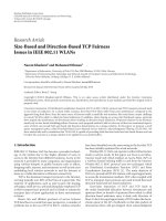
Involved BS
Not involved BS
MS
Hyperbolas of constant TDoA
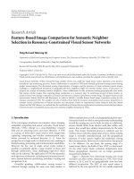
Figure 1: TDoA positioning in cellular networks with N
BS
= 4 in-
volved BSs.
functions (CDFs). They show the potential of this algorithm

in terms of accuracy and computational complexity, outper-
forming the GN method in cellular networks. Furthermore,
a performance comparison with the noniterative Chan-Ho
(CH) method [17] is given. Note that the CDFs are an im-
portant benchmark in the context of the FCC-E911 require-
ments. This paper paves the way for a general processing of
all kinds of measurements under the joint framework of FGs
for future research.
Throughout this paper, vectors and matrices are denoted
by lower- and uppercased bold letters. The matrix I
n
is the
n
× n identity matrix, the matrix 0
n×m
is the n × m matrix
with zeros, the operation “
⊗” denotes the Kronecker prod-
uct, E
{·} denotes expectation, (·)
T
denotes transpose, and
·
2
denotes the Euclidean norm.
2. SYSTEM MODEL
The time-synchronized BSs are organized in a cellular
network with cell radius R according to Figure 1. For non-
synchronized BSs, the so-called location measurement units
(LMUs) are u sed for processing. The LMUs are associated to

the BSs and compensate the missing synchronization of the
BS network. The MS is located at x
= [x, y]
T
and only the
N
BS
nearest BSs at x
μ
, μ ∈{1, 2, , N
BS
} are used for posi-
tioning. The distance between the BSs and the MS is given
by
r
μ
(x) =


x
μ
− x


2
=


x
μ

− x

2
+

y
μ
− y

2
. (1)
This equation can also be seen as a result of ToA measure-
ments. With ToA, the absolute time for a signal traveling
from the BS to the MS or vice versa is measured. It is not
even required that all BSs be synchronized with each other,
additionally synchronized time knowledge, that is, the time
of transmission, is necessary at the MS. In case that no exact
time knowledge is available (time offset of the MS), an ad-
ditional BS is necessary to estimate this offset according to
the ToA principle as it is used in GNSSs [6, 7]. Also round-
trip delay (RTD) procedures can be chosen to obtain ToAs
independent of any synchronization assumptions. But this
procedure has the drawback that measurements have to be
performed in both uplink and downlink. The propagation
time from the BSs to the MS is proportional to the distance.
Hence, we get the distance b etween the MS and all involved
BSs. From a geometrical point of view, the MS lies on circles
around the BSs. The intersection of these circles gives the po-
sition of the terminal.
The problem of processing ToA measurements is the fact

that the MS is usually not synchronized to the BSs, and
therefore an additional BS is required to estimate the time
offset. To avoid this drawback, the TDoAs measure directly
the time difference of signals received from various BSs [2, 3],
that is, the unknown time offset of the MS with respect to the
synchronized BSs is not relevant for TDoA processing. In the
geometrical interpretation, the MS lies on hyperbolas with
foci at the two related BSs (cf. Figure 1). The intersection
gives the position of the MS. Note that TDoAs are defined
with respect to an arbitrary chosen reference BS.
In the following, we treat distances and propagation
times as equivalent, and thus the TDoAs for BS ν
∈
{
2, 3, , N
BS
} with respect to BS 1 can be wr itten as
d
ν,1
(x) = r
ν
(x) − r
1
(x), (2)
where—without loss of generality—we use BS 1 as the refer-
ence BS. The N
BS
−1 linear independent TDoAs compose the
vector
d(x)

=

d
2,1
(x), d
3,1
(x), , d
N
BS
,1
(x)

T
,(3)
and the corresponding TDoA measurements are given by
d
=

d
2,1
, d
3,1
, , d
N
BS
,1

,(4)
based on the measurement model
d

= d(x)+n,(5)
where
n
=

n
2,1
, , n
N
BS
,1

T
(6)
is zero-mean additive white Gaussian noise (AWGN) [3]with
covariance matrix
Σ
n
= E

nn
T

. (7)
For the solution of the estimation problem for the MS
location, it is a common way to follow the weighted nonlin-
ear least-squares approach [3, 12] which minimizes the cost
function
ε(x)
=


d − d(x)

T
Σ
−1
n

d − d(x)

(8)
C. Mensing and S. Plass 3
with respect to the unknown MS position x yielding
x = argmin
x
ε(x). (9)
In the general case, there exists no closed-form solution to
the nonlinear two-dimensional optimization problem given
by (9), and hence iterative approaches are necessary. A stan-
dard approach to deal with (9) is based on the GN algorithm
[3, 18]. The GN algorithm linearizes the system model in (5)
about some initial value x
(0)
yielding
d(x)
≈ d

x
(0)


+ Φ(x)


x=x
(0)

x − x
(0)

, (10)
with the elements of the (N
BS
− 1) × 2Jacobianmatrix
Φ(x)
=∇
T
x
⊗ d(x)
=
⎡
⎢
⎢
⎢
⎢
⎢
⎢
⎢
⎢
⎢
⎢

⎢
⎣
x − x
2
r
2
−
x − x
1
r
1
y − y
2
r
2
−
y − y
1
r
1
x − x
3
r
3
−
x − x
1
r
1
y − y

3
r
3
−
y − y
1
r
1
.
.
.
.
.
.
x
− x
N
BS
r
N
BS
−
x − x
1
r
1
y − y
N
BS
r

N
BS
−
y − y
1
r
1
⎤
⎥
⎥
⎥
⎥
⎥
⎥
⎥
⎥
⎥
⎥
⎥
⎦
,
(11)
where
∇
x
= [∂/∂x, ∂/∂y]
T
. Afterwards, using (10)and(8),
the linear least-squares procedure is applied resulting in the
iterated solution

x
(k+1)
= x
(k)
+

Φ
T

x
(k)

Σ
−1
n
Φ

x
(k)

−1
·Φ
T

x
(k)

Σ
−1
n


d − d

x
(k)

=
x
(k)
+ A
(k),−1
g
(k)
.
(12)
The GN algorithm provides very fast convergence and accu-
rate estimates for good initial values. For poor initial values
and bad geometric conditions the algorithm results in a rank-
deficient, and thus noninvertible matrix A
(k)
for certain con-
stellations of MS a nd BSs. In this case, the algorithm diverges
[13]. However, a more accurate initial estimate, for example,
from a one-step linear least-squares solution as shown in [2],
can reduce the divergent behavior of the GN algorithm.
Note that an asymptotically efficient maximum-likeli-
hood (ML) approach to cover this MS positioning problem
is not possible in a real-time scenario due to computational
complexity. However, we will use the ML solution as refer-
ence for the simulation results.

The performance bound for the proposed scenario is
given by the Cramer-Rao lower bound (CRLB) [12]for
TDoA defined as
CRLB(x) = CRLB
TDoA
(x) =

trace

Φ
T
(x)Σ
−1
n
Φ(x)

−1
(13)
for each MS position where the subscript TDoA is omitted in
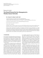
the following for the sake of simplification. Ne vertheless, we
are interested in the positioning accuracy for all possible MS
0
0.1
0.2
0.3
0.4
0.5
CRLB (km)
00.05 0.10.15 0.20.25 0.3
σ

n
(km)
N
BS
= 3, TDoA
N
BS
= 3, ToA
N
BS
= 3, TDoA + ToA
N
BS
= 4, TDoA
N
BS
= 4, ToA
N
BS
= 4, TDoA + ToA
N
BS
= 5, TDoA
N
BS
= 5, ToA
N
BS
= 5, TDoA + ToA
Figure 2: CRLB versus σ

n
for different positioning methods, R =
3km.
locations in the cellular network. Thus, we introduce
CRLB = E
x

CRLB(x)

(14)
as mean value of the bound for the w hole network.
Figure 2 shows the CRLB for TDoA, ToA, and joint
TDoA and ToA measurements. The CRLB for ToA is given
as
CRLB
ToA
(x) =

trace

Ψ
T
(x)Σ
−1
n,ToA
Ψ(x)

−1
, (15)
with

Ψ(x)
=∇
T
x
⊗ r(x) =
⎡
⎢
⎢
⎢
⎢
⎢
⎢
⎢
⎢
⎢
⎢
⎢
⎣
x − x
1
r
1
y − y
1
r
1
x − x
2
r
2

y − y
2
r
2
.
.
.
.
.
.
x
− x
N
BS
r
N
BS
y − y
N
BS
r
N
BS
⎤
⎥
⎥
⎥
⎥
⎥
⎥

⎥
⎥
⎥
⎥
⎥
⎦
, (16)
where
r(x)
=

r
1
(x), r
2
(x), , r
N
BS
(x)

T
, (17)
and Σ
n,ToA
is the covariance matrix of the noise for ToA mea-
surements. Equivalently, the CRLB for joint TDoA and ToA
measurements can be calculated as
CRLB
TDoA + ToA
(x)

=





trace

Φ (x)
Ψ (x)

T

Σ
n
0
0 Σ
n,ToA

−1

Φ (x)
Ψ (x)

−1
.
(18)
4 EURASIP Journal on Advances in Signal Processing
For the simulations, we assume that the noise v ariance is the
same for each measurement, that is, we use Σ

n
= σ
2
n
I
N
BS
−1
(perfect power control). It should be pointed out that for ToA
and also joint TDoA + ToA procedures (Figure 2), the CRLB
can be achieved with simple methods, for example, based on
the GN algorithm. However, for TDoA with the hyperbolic
character of the measurements, the effort to the algorithms
is much higher to achieve CRLB over the whole network and
more sophisticated methods—as in the following proposed
FG-based approach—are necessary.
Note that all considered algorithms in this paper are not
restricted to any assumptions about the source of the mea-
surements. They work for both uplink and downlink mea-
surements and are independent of the underlying wireless
cellular network.
3. POSITIONING BASED ON FACTOR GRAPHS
Historically, FGs as a generalization of Tanner graphs come
from coding theory and were used for decoding of low-
density parity check (LDPC) or concatenated (turbo) codes.
But additionally, there exist a lot of algorithms which can be
described in an FGs framework [19], for example, Kalman
filters or Fourier transforms. In [14, 15], Chen et al. pro-
posed a method for solving the positioning problem in an
FGs environment using ToA measurements. In [16], they

extended their method to AoA measurements. In this sec-
tion, we present the solution for FG-based positioning using
TDoA measurements with—compared to ToA and AoA—
their more complicated hyperbolic character. In the follow-
ing, we give a short overview of basic principles regard-
ing FGs theory. Afterwards, we describe necessary geometric
fundamentals for the proposed procedure. Finally, the TDoA
positioning algorithm using FGs is derived in detail.
3.1. Factor graphs and the sum-product algorithm
An FG is a bipartite graph that in its original sense can de-
scribe the structure of a factorization [19]. If we assume as
an example the function f (x
1
, x
2
, x
3
, x
4
)whichcanbefactor-
ized in
f

x
1
, x
2
, x
3
, x

4

= f
1

x
1

f
2

x
1
, x
2
, x
3

f
3

x
3
, x
4

, (19)
the structure of this fac torization can be expressed by an FG.
The bipartite FG consists of variable nodes for each var iable
x

ν
occurring in the function, factor nodes for each local func-
tion f
μ
of f , and edges connecting var iable nodes x
ν
with
factor nodes f
μ
, if and only if x
ν
is a function of f
μ
[19]. The
corresponding FG for the example (cf. (19)) can be seen in
Figure 3.
Often, we are interested in a marginalization of such a
structured function, that is, to find a function only depend-
ing on one of the unknowns describing for example the ex-
trinsic soft information in a decoding framework. A s ystem-
atic way to do so is the application of the so-called sum-
product algorithm (SPA). It is a message passing algorithm
working on the FG. There is no general assumption about
these messages, for example, they can take the form of soft
f
1
x
1
f
2

x
2
x
3
f
3
x
4
Figure 3: Example for a factor graph.
information or probability density functions (PDFs). For ex-
ample, in a decoding scenario of Hamming codes, the factor
nodes describe the parity check constraints and the messages
passed in the FG consist of the extrinsic soft information.
In the following, we describe the fundamental rules of
the SPA and refer to [19] for more details. Generally, we dif-
ferentiate between messages passed from variable nodes to
factor nodes a nd vice versa. According to the SPA, a message
passing from a variable node x to a factor node f should be
calculated as
L
x→ f
(x) =

h∈n(x)\{ f }
L
h→x
(x), (20)
where n(x) denotes the set of neighbors of a given node x in
the FG. Note that the product in (20) should be interpreted
in a more abstract way, depending on type and structure of

the messages. The rule for computing a message from local
node f to variable node x is given as
L
f →x
(x) =

∼{x}

f (X)

y∈n( f )\{x}
L
y→ f
(y)

, (21)
with the set of arguments of the function f defined as X
=
n( f ), and the so-called summary operator

∼{x}
indicating
the variables being not summed over. With these two rules—
after an initialization step for the nodes at the edges—all
messages in the FG can be calculated step by step. For the
final calculation of the marginalization of the variables, we
use the termination rule
L(x)
=


h∈n(x)
L
h→x
(x), (22)
that is, the multiplication of all incident messages to this vari-
able node, depending only on one variable.
Generally, it is differentiated between FGs with and with-
out cycles. For cycle-free FGs, the optimum performance—
depending on the quality criterion—can be achieved, but for
FGs with cycles only an approximation of the optimum so-
lution is obtained. Besides, in case of FGs with cycles usually
adequate scheduling algorithms are necessary to determine
the messages in a specific order. Nevertheless, there often ex-
ists no optimum classical solution or it is a ssociated with too
high computational complexity (cf. LDPC or turbo codes).
Therefore, a solution based on an FG with cycles may be the
only reasonable way to deal with the problem.
C. Mensing and S. Plass 5
−4
−3
−2
−1
0
1
2
3
4
y
−4 −3 −2 −10 1 2 3 4
x

MS
BS
Hyperbola of constant TDoA
Hyperbola after rotation (32)
Hyperbola after shift operation (34)
Figure 4: Hyperbola processing.
3.2. Geometric fundamentals
To derive the algorithm of TDoA-based positioning using
FGs, we need some fundamental calculus taken from the-
ory of conic sections and shown in the following. The aim of
this procedure is to provide the local constra ints of the factor
nodes in the FG. The idea is to process x and y coordinates
mostly independent. Information is only exchanged at the
so-called mapping factor nodes. From a geometric point of
view, the proceeding is based on a principal a xis transforma-
tion by rotation, a shift operation, and finally the mapping
operation where the original hyper bola equation is trans-
formed in a suitable way for FG processing.
As first step, each TDoA equation (2)—under assump-
tion of the measurement model defined in (5)—can be
rewritten as
a
ν,11
x
2
+ a
ν,22
y
2
+


a
ν,12
+ a
ν,21

xy
+

a
ν,01
+ a
ν,10

x +

a
ν,02
+ a
ν,20

y
+ a
ν,00
= 0
(23)
for all N
BS
− 1 TDoAs, using simple algebraic operations.
Note that due to squaring operations a second hyperbola

branch—compared to the original TDoA equation (2)—
appears (cf. Figure 4), where the MS does not lie on. Never-
theless, this ambiguity can be resolved by observing the signs
of the corresponding TDoAs and does not restrict the perfor-
mance of the later derived algorithm. The coefficients a
ν,ij
,
i, j
∈{0, 1, 2},in(23) can simply be computed in depen-
dence on the known BS positions and measurements. The
quadratic equation (23) can be written in matrix-vector no-
tation resulting in
x
T
A
ν
x + a
T
ν
x + a
ν,00
= 0 (24)
for all ν
∈{2, 3, , N
BS
} TDoAs related to reference BS 1,
using the quadratic form x
T
A
ν

x with
A
ν
=

a
ν,11
a
ν,12
a
ν,21
a
ν,22

(25)
and the vector
a
ν
=

a
ν,10
, a
ν,20

T
. (26)
Equation (24) can be diagonalized by application of an eigen-
value decomposition of the matrix
A

ν
= U
ν
Λ
ν
U
T
ν
, (27)
where
Λ
ν
=

λ
ν,1
0
0 λ
ν,2

(28)
is the diagonal matrix composed of the eigenvalues, and
U
ν
=

u
ν,1
u
ν,2


(29)
is a unitary matrix with the corresponding eigenvectors. For
later purposes, we choose the order of the eigenvalues in such
a way that
sign

λ
ν,1

sign

B
ν

=
1 (30)
is fulfilled, w here
B
ν
= a
T
ν
U
ν
Λ
−1
ν
U
T

ν
a
ν
− a
ν,00
. (31)
With the substitution
x = U
ν
x

ν
(32)
in (24)—describing the rotation—we obtain

x

ν

T
Λ
ν
x

ν
+ a
T
ν
U
ν

x

ν
+ a
00
= 0, (33)
that is, a diagonalized system which can be seen as the origi-
nal system in a new coordinate plan (cf. Figure 4). In a second
step, the rotated hyperbola is shifted around the origin. For
this purpose, we have to differentiate between two cases de-
pending on the character of the eigenvalues. In the first case
(λ
ν,1
/= 0, λ
ν,2
/= 0), we can do the second substitution (shift
operation)
x

ν
= x

ν
−
1
2
Λ
−1
ν
U

T
ν
a
ν
(34)
in (33), yielding the hyperbola equation in main position (cf.
Figure 4)givenas

x

ν

T
B
ν
x

ν
− 1 = 0, (35)
with
B
ν
=
⎡
⎢
⎢
⎣
B
ν
λ

ν,1
0
0
B
ν
λ
ν,2
⎤
⎥
⎥
⎦
. (36)
6 EURASIP Journal on Advances in Signal Processing
Note that
sign

B
ν

=

10
0
−1

(37)
is always valid by construction (30) which confirms the
hyperbolic character. In case that one eigenvalue is equal to
zero (by construction: λ
ν,1

/= 0, λ
ν,2
= 0), the two hyperbola
branches degenerate into a line, yielding the other case of the
second substitution
x

ν
=
⎡
⎢
⎢
⎣
x

ν
−
a
T
ν
u
ν,1
2λ
ν,1
y

ν
⎤
⎥
⎥

⎦
, (38)
and the degenerated hyperbola equation becomes

x

ν

2
= 0. (39)
This case occurs if the corresponding TDoA is equal to zero.
Note that the case that both eigenvalues are equal to zero is
not relevant for realistic BSs and MS constellations.
As last step, we define a mapping operation which will be
used in the mapping factor nodes of the FG to exchange in-
formation in x and y directions. According to (35), we define
x

ν
=±

λ
ν,1
B
ν
−
λ
ν,1
λ
ν,2


y

ν

2
,
y

ν
=±

λ
ν,2
B
ν
−
λ
ν,2
λ
ν,1

x

ν

2
.
(40)
3.3. TDoA positioning algorithm based on

factor graphs
The aim of this positioning algorithm using FGs is to de-
termine the location of the MS by processing the measured
TDoAs with their statistic properties and the known BS po-
sitions. It breaks down the general high-complex problem
in several low-complex subproblems that can be solved in
a distributed way and finds the solution—starting with an
initial guess—iteratively. The corresponding FG is depicted
in Figure 5. The factor nodes are given by the substitution
and mapping operations defined in the previous section (see
(32), (33), and (34)) and can be seen as constraint nodes
among the variables. The rotation (R) and shift (S) opera-
tions process the messages of x and y coordinates indepen-
dently. In the mapping (M) n odes, information between x
and y coordinates is exchanged. The messages that are passed
around the FG are defined as PDFs for the corresponding
variables in the variable nodes. In our investigations, we as-
sume Gaussian distributions for these PDFs according to
N

x, m, σ
2

∼ exp

−
(x − m)
2
2σ
2


, (41)
for a random variable x with mean value m and variance σ
2
.
This assumption simplifies the calculations performed by the
x
R
x
2
R
x
N
BS
y
R
y
2
R
y
N
BS
x

2
x

N
BS
y


2
y

N
BS
S
x
2
S
x
N
BS
S
y
2
S
y
N
BS
x

2
x

N
BS
y

2

y

N
BS
M
xy
2
M
xy
N
BS
Figure 5: Factor graph for TDoA positioning.
SPA considerably. After the initialization of the FG in a suit-
able way [15], the rules of SPA can be applied straightfor-
wardly. Furthermore, in our derivation we need two general
rules [19] for random variables with Gaussian distributions.
At first, the relation
N

n=1
N

x, m
n
, σ
2
n

∼ N


x, m
P
, σ
2
P

(42)
holds, where the mean value of the resulting Gaussian distri-
bution can be calculated as
m
P
= σ
2
P
N

n=1
m
n
σ
2
n
, (43)
and the variance is given as
σ
2
P
=
1


N
n
=1
1/σ
2
n
. (44)
Secondly, we will make use of the integ ration r ule

∞
x=−∞
N

x, m
1
, σ
2
1

N

y, αx + m
2
, σ
2
2

dx
∼ N


y, αm
1
+ m
2
, α
2
σ
2
1
+ σ
2
2

.
(45)
In the following, we show the necessary message pass-
ing oper ations. Note that the iteration index is omitted here
for the sake of simplification and that the summary operator
(cf. (21)) is replaced by an integration operator due to the
Gaussian character of the messages. We start at the messages
passed from the variable node x to factor n odes R
x
ν
.Accord-
ing to SPA, we obtain
L
x→R
x
ν
(x) ∼


μ/=ν
L
R
x
μ
→x
(x), (46)
C. Mensing and S. Plass 7
that is, the multiplication of all incident messages which can
be calculated using (42). For the messages from the factor
nodes R
x
ν
to the variable nodes x

ν
, information about R
x
ν
is
essential. This is given by the rotation (R) operation as first
substitution (32), and under assumption of Gaussian distri-
butions, we obtain
f
R
x
ν

x, x


ν

∼ N

x

ν
, u
T
ν,1
x, σ
2
x

ν

(47)
as constraint rule for the factor node where the variance is
set to the variance in x-direction of the noisy observations,
that is, σ
2
x

ν
= σ
2
x
which can be derived from (7)[15]. The SPA
yields

L
R
x
ν
→x

ν

x

ν

∼

∞
x=−∞
f
R
x
ν

x, x

ν

L
x→R
x
ν
(x)dx, (48)

which can be computed with (45). We proceed by calculating
the messages to the shift operation (S) factor node, simply
given as
L
x

ν
→S
x
ν

x

ν

=
L
R
x
ν
→x

ν

x

ν

. (49)
The messages from the shift operation nodes S

x
ν
with the con-
straint (cf. (34))
f
S
x
ν

x

ν
, x

ν

∼ N

x

ν
, x

ν
+
1
2λ
ν,1
u
T

ν,1
a
ν
, σ
2
x

ν

(50)
to the variable nodes x

ν
(σ
2
x

ν
= σ
2
x
) are obtained by
L
S
x
ν
→x

ν


x

ν

∼

∞
x

ν
=−∞
f
S
x
ν

x

ν
, x

ν

L
x

ν
→S
x
ν


x

ν

dx

ν
(51)
using (45). The messages to the mapping (M) nodes M
xy
ν
can
simply be calculated as
L
x

ν
→M
xy
ν

x

ν

=
L
S
x

ν
→x

ν

x

ν

. (52)
A very important node is the mapping node, where informa-
tion between x and y coordinates is exchanged. It is based
on the mapping operations defined in (40), but to fulfil the
Gaussian assumption in the corresponding factor node, a
Gaussian approximation similar as that shown in [15]has
to be performed. Additionally, several cases due to sign am-
biguities have to be distinguished. Thus, in this paper we give
only the general formula according to SPA obtained by
L
M
xy
ν
→y

ν

y

ν


∼

∞
x

ν
=−∞
f
M
xy
ν

x

ν
, y

ν

L
x

ν
→M
xy
ν

x

ν


dx

ν
,
(53)
where f
M
xy
ν
(x

ν
, y

ν
) describes the mapping constraint (40).
The necessary message calculations from the mapping nodes
back to the variable nodes x and y and the processing in the y
branch of Figure 5 correspond to the steps described above.
After initialization, the messages are calculated iteratively up
to convergence. We emphasize that due to the Gaussian char-
acter of the messages and the possibility of distributed com-
puting, the processing effort is limited to simple operations.
−1
0
1
2
3
4

5
6
7
8
9
10
y (km)
0246810
x (km)
BS
MS
Initial position value
Estimated position after first interation
Estimated position after second interation
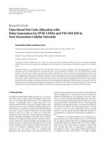
Figure 6: Example for the FG positioning algori thm with N
BS
= 3
BSs.
In a final termination step, the marginalization of the coor-
dinate variable nodes x and y can easily be computed by
L(x)
=

ν
L
R
x
ν
→x
(x) (54)

for the x coordinate. The final estimates
x = x
(K)
after K
iteration steps are given by the mean values of the Gaussian
distributions according to (54). Note that also the var iances
in x and y directions are provided by the algorithm.
We are aware of the fact that the here proposed FG has
cycles, and therefore the estimates are only an approxima-
tion of the optimum solution. But simulation results show
the near-optimum behavior of the algorithm for the general
scenario considered in this paper. Analytical investigations
on the convergence behavior of this FG with cycles are hard
to establish because the occurring cycles are very short.
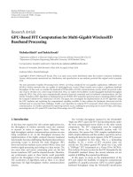
3.4. Implementation example
To demonstrate the functionality of the FG-based position-
ing algorithm, we show a simple example with N
BS
= 3 in-
volved BSs at x
1
= [0, 0]
T
, x
2
= [0, 9]
T
,andx
3
= [10, 2]

T
(cf. Figure 6). Hence, two TDoA measurements for the MS
at x
= [3, 3]
T
are available that can be calculated as d(x) =
[2.47, 2.83]
T
. The noise vector for these measurements is
given as n
= [0.2, −0.2]
T
with variances in x-andy-compo-
nents as σ
2
x
= σ
2
y
= 0.1, and the initial value is at x
(0)
=
[4, 4]
T
.
In the following, we describe the required calcula-
tions in more detail for this example. For processing the
8 EURASIP Journal on Advances in Signal Processing
x-components of the first TDoA measurement, we need the
matrix and vector

A
1
=

7.11 0
0
−73.89

, a
1
= [0, 665.05]
T
. (55)
The resulting eigenvalues are λ
1,1
=−73.89 and λ
1,2
= 7.11,
and the eigenvector for the x-component is u
1,1
= [0, 1]
T
.
Finally, the scalar value B
1
=−131.26 is required.
With this information, we can star t the algorithm in the
previous section. It is initialized with
L
x→R

x
2
(x) ∼ N (x,4,0.1), (56)
that is, for the x-component the message from the variable
node x to the factor node R
x
2
includes in the first step a Gaus-
sian distribution with mean value as the x-component of the
initial value x
(0)
, a nd an assumed variance of σ
2
x
= 0.1. With
knowledge of the eigenvectors, the constraint rule for the ro-
tation factor node is given as
f
R
x
2

x, x

2

∼ N

x


2
,4,0.1

. (57)
Hence, the merged Gaussian distributions for the message
from the rotation factor node to the variable node x

2
can be
calculated as
L
R
x
2
→x

2

x

2

∼ N

x

2
,8,0.2

, (58)

where we have used the relation in (45)withα
= 1. The mes-
sage to the shift factor node is simply given as
L
x

2
→S
x
2

x

2

=
L
R
x
2
→x

2

x

2

∼ N


x

2
,8,0.2

. (59)
Similar to the rotation rule, the shift rule can be calculated as
f
S
x
2

x

2
, x

2

∼ N

x

2
, −6.5, 0.1

, (60)
which is further used to calculate the message to the variable
node x


2
.Weobtain
L
S
x
2
→x

2

x

2

∼ N

x

2
,1.5, 0.3

, (61)
again using (45). The messages to the mapping factor node
are simply
L
x

2
→M
xy

2

x

2

= L
S
x
2
→x

2

x

2

∼ N

x

2
,1.5, 0.3

. (62)
Using (40), the mean value for the mapping node can be cal-
culated as 3.36. The corresponding var iance is given as 0.17.
Hence, we obtain
L

M
xy
2
→y

2

y

2

∼ N

y

2
,3.36, 0.17

. (63)
On the backward step from y

2
to y, the described operations
are very similar, and we end up at
L
R
y
2
→y
(y) ∼ N (y,3.16, 0.36). (64)

Calculating the values from y to x for the first TDoA mea-
surement, we obtain
L
R
x
2
→x
(x) ∼ N (x,3.86, 0.41). (65)
The values for the second TDoA can be computed as
L
R
y
3
→y
(y) ∼ N (y,3.36, 0.32),
L
R
x
3
→x
(x) ∼ N (x,2.58, 0.31).
(66)
With these messages, mean value and variance of the esti-
mated position can be calculated using relation (42). This
yield the improved estimation after the first iteration
x
(1)
∼ N

x,


3.19
3.28

,

0.18
0.17

. (67)
Of course, more iterations can be performed to further im-
prove the performance (cf. Figure 6).
4. SIMULATION RESULTS
We test the proposed algorithms in a cellular network with
cell radius R
= 3 km and assume constant noise power for all
involved links from the BSs to the MS, that is, Σ
n
= σ
2
n
I
N
BS
−1
.
Figures 7–9 show CRLB(x) (cf. (13)) using N
BS
=
{

3, 4, 5} for positioning. We obser ve that, for example, for
N
BS
= 3 near the BSs and on the links between the BSs the
positioning performance is restricted due to geometric con-
stellation. In these cases, we can expect limited perfor mance
of the algorithms. We further can see that the performance
increases when more BSs are involved in the localization pro-
cess.
In Figure 10, the performance of the investigated algo-
rithmsisanalyzedforN
BS
= 3andσ
n
= 0.2 km. Initial value
for the iterative algorithms is the mean value of the positions
of all involved BSs, that is,
x
(0)
=
1
N
BS
N
BS

ν=1
x
ν
. (68)

We comp are
CRLB (cf. (14)) with the achievable RMSE for
the algorithms defined as
RMSE
=

E
x


x − x
2
2

≥
CRLB (69)
and averaged over several MS positions and noise realiza-
tions, where
x = x
(K)
is the estimate provided by the iterative
algorithms after K iteration steps. The GN algorithm pro-
vides very fast convergence and accurate estimates for good
initial values. For poor initial values and bad geometric con-
ditions (e.g., at the cell edge or near the BSs), the algorithm
diverges [13]. Therefore, in these cases, the resulting estimate
is set to
x = x
(0)
to show the loss with respect to CRLB. Any-

way, for perfect conditions, GN provides fast convergence.
The FG algorithm converges after K
FG
= 8iterationstepsand
reaches nearly
CRLB. Additionally, in Figure 10 the needed
floating point operations (FLOPs) as measure for compu-
tational complexity are depicted for both algorithms. Obvi-
ously, FG offers a better performance compared to GN by just
slightly increased complexity.
Figure 11 shows a performance comparison of the FG
algorithm for various numbers of involved BSs. It can be
C. Mensing and S. Plass 9
−6
−4
−2
0
2
4
6
y (km)
0.1
0.11
0.12
0.13
0.14
0.15
CRLB (x)(km)
−6 −4 −20 2 4 6
x (km)

BS
Figure 7: CRLB(x)forσ
n
= 0.1 km, R = 3km,N
BS
= 3.
−6
−4
−2
0
2
4
6
y (km)
0.082
0.083
0.084
0.085
0.086
0.087
0.088
0.089
0.09
0.091
0.092
CRLB (x)(km)
−6 −4 −20246
x (km)
BS
Figure 8: CRLB( x)forσ

n
= 0.1km,R = 3km,N
BS
= 4.
−6
−4
−2
0
2
4
6
y (km)
0.0715
0.072
0.0725
0.073
0.0735
0.074
0.0745
0.075
0.0755
0.076
CRLB (x)(km)
−6 −4 −20 2 4
6
x (km)
BS
Figure 9: CRLB( x)forσ
n
= 0.1km,R = 3km,N

BS
= 5.
0
0.1
0.2
0.3
0.4
0.5
RMSE (km)
0
5
10
15
20
25
×10
2
FLOPs
0 5 10 15
Iteration k
RMSE, GN
RMSE, FG
CRLB
FLOPs, GN
FLOPs, FG
Figure 10: RMSE and FLOPs versus iterations for σ
n
= 0.2km,R =
3km,N
BS

= 3.
0
0.1
0.2
0.3
0.4
0.5
RMSE (km)
00.05 0.10.15 0.20.25 0.3
σ
n
(km)
N
BS
= 3, CH
N
BS
= 3, FG
N
BS
= 3, CRLB
N
BS
= 4, CH
N
BS
= 4, FG
N
BS
= 4, CRLB

N
BS
= 5, CH
N
BS
= 5, FG
N
BS
= 5, CRLB
Figure 11: RMSE versus σ
n
for FG and CH algorithms, R = 3km.
seen that the deviation from CRLB is very small, even for
N
BS
= 3 and high noise power. To get a better assessment
for the performance of the iterative FG algorithm, the re-
sults are also compared with a noniterative solution which
is based on a method invented by Chan and Ho [17]. It is
a three-step procedure extending the spher ical interpolation
10 EURASIP Journal on Advances in Signal Processing
method [20] and achieving CRLB for low noise power, but
with restricted accuracy for higher noise power. The number
of required FLOPs is similar compared to the FLOPs for FG
with K
FG
= 8, but we can observe that the performance of
the Chan-Ho (CH) method—especially in the most interest-
ing case of N
BS

= 3—is considerably worse.
We are also interested in CDFs for investigating the per-
formance of the algorithms in general cellular networks. In
Figure 12, the performance of GN, FG, and ML as the refer-
enceboundisanalyzedforN
BS
= 4 and different values for
the noise power σ
n
. Note that the quality of the initial value
strongly depends on the different MS positions in the cellular
network. The estimation error is defined as
ε
=


x − x


2
, (70)
where
x is again the final estimate of the algorithms after
convergence. The CDF shows the probability that the esti-
mation error ε is below a fixed value ε
err
, a veraged over sev-
eral MS positions a nd noise realizations. We observe that FG
outperforms the standard GN algorithm for the complete
range. However, there is still a gap between FG and the ML

bound. This can be explained by observing the CRLB plots
(e.g., Figure 8) with the geometric constellations, bad initial
values for certain MS positions, and the cycles in the FG.
However, the performance difference between GN and ML
bounds is much bigger than between FG and ML bounds.
Hence, the FG can also in terms of CDFs be seen as more ro-
bust against bad geometric constellations and bad inaccurate
initial values. Additionally, the FCC rule for emergency calls
is shown in Figure 12 (dotted lines). According to the FCC
requirements for locating emergency callers, 67% of the posi-
tions have to be estimated with an error which is smaller than
0.1 km for network initiated positioning. We see that GN is
not suitable to achieve this requirement for σ
n
= 0.1km,
whereas FG fulfils the FCC rule for this scenario.
Figure 13 shows the performance of the FG algorithm in
dependence on the number of used BSs for σ
n
= 0.1km.
Clearly, for increasing N
BS
, also the performance improves.
Additionally, the difference between FG and ML gets smaller
for increasing N
BS
. Note that for the simulated scenario, at
least N
BS
= 4 BSs are required to fulfil the FCC requirement.

5. CONCLUSIONS
In this paper, we analyzed the mobile station positioning per-
formance in wireless cellular networks using time difference
of arrival measurements in a new factor graphs framework.
In this scenario, the standard Gauss-Newton algorithm—
with similar computational complexity properties—diverges
for inaccurate initial v alues and bad geometric conditions.
To avoid these drawbacks, we propose to use a more ro-
bust time difference of arrival positioning algorithm based
on factor g raphs. Simulation results in terms of root-mean-
square errors and cumulative density functions show that
this method is suitable to estimate the mobile station loca-
tion with high accuracy and moderate complexity. The pro-
0
0.1
0.2
0.3
0.4
0.5
0.6
0.7
0.8
0.9
1
CDF, P (ε<ε
err
)
00.05 0.10.15 0.20.25 0.3
ε
err

(km)
GN, σ
n
= 0.05 km
FG, σ
n
= 0.05 km
ML, σ
n
= 0.05 km
GN, σ
n
= 0.1km
FG, σ
n
= 0.1km
ML, σ
n
= 0.1km
GN, σ
n
= 0.15 km
FG, σ
n
= 0.15 km
ML, σ
n
= 0.15 km
Figure 12: CDF for different algorithms, R = 3km,N
BS

= 4.
0
0.1
0.2
0.3
0.4
0.5
0.6
0.7
0.8
0.9
1
CDF, P (ε<ε
err
)
00.05 0.10.15 0.20.25 0.3
ε
err
(km)
FG, N
BS
= 3
ML, N
BS
= 3
FG, N
BS
= 4
ML, N
BS

= 4
FG, N
BS
= 5
ML, N
BS
= 5
Figure 13: CDF for different numbers of BSs, R = 3km, σ
n
=
0.1km.
posed method is very close to the Cramer-Rao lower bound
and outperforms also the noniterative Chan-Ho algorithm.
Furthermore, the performance difference between the fac-
tor graphs approach and the optimum—but computational
prohibitive—maximum-likelihood solution is very small for
various parameters, and thus the proposed algorithm allows
the adherence to the FCC emergency call requirements over
amoreextendedrange.
C. Mensing and S. Plass 11
ACKNOWLEDGMENT
The material in this paper was presented in part at the IEEE
Symposium on Personal, Indoor, and Mobile Radio Com-
munications (PIMRC), Helsinki, Finland, September 2006.
REFERENCES
[1] J.J.Caffery, Wireless Location in CDMA Cellular Radio Systems,
Kluwer Academic Publishers, Boston, Mass, USA, 2000.
[2] A. H. Sayed, A. Tarighat, and N. Khajehnouri, “Network-based
wireless location: challenges faced in developing techniques
for accurate wireless location information,” IEEE Signal Pro-

cessing Magazine, vol. 22, no. 4, pp. 24–40, 2005.
[3] F. Gustafsson and F. Gunnarsson, “Mobile positioning using
wireless networks: possibilities and fundamental limitations
based on available wireless network measurements,” IEEE Sig-
nal Processing Magazine, vol. 22, no. 4, pp. 41–53, 2005.
[4] Federal Communications Commission (FCC), FCC 99-245:
Third Report and Order. October 1999, />911/enhanced/.
[5] Coordination Group on Access to Location Information for
Emergency Services (CGALIES), Final Report: Report on Im-
plementation Issues Related to Access to Location Information
by Emergency Services (E112) in the European Union. Febru-
ary 2002, />[6] B. W. Parkinson and J. J. Spilker Jr., Global Positioning System:
Theory and Applications, Volume 1, vol. 163 of Progress in As-
tronautics and Aeronautics, American Institute of Aeronautics
& Astronautics, Reston, Va, USA, 1996.
[7] P.MisraandP.Enge,Global Positioning System: Signals, Mea-
surements and Performance, Ganga-Jamuna Press, Lincoln,
Mass, USA, 2004.
[8] R. Ercek, P. De Doncker, and F. Grenez, “Study of pseudo-
range error due to non-line-of-sight-multipath in urban
canyons,” in Proceedings of the 18th International Technical
Meeting of the Satellite Division of the Institute of Navigation
(ION GNSS ’05), pp. 1083–1094, Long Beach, Calif, USA,
September 2005.
[9] Y. Zhao, “Standardization of mobile phone positioning for 3G
systems,” IEEE Communications Magazine,vol.40,no.7,pp.
108–116, 2002.
[10] IST-2003-507581, WINNER Project. -winner
.org/.
[11] IST-2003-507581, WINNER Deliverable D4.8.1: WINNER II

Intramode and Intermode Cooperation Schemes Definition.
June 2006, />[12] S. M. Kay, Fundamentals of Statistical Signal Processing: Esti-
mation Theory, Prentice-Hall, Upper Saddle River, NJ, USA,
1993.
[13] C. Mensing and S. Plass, “Positioning algorithms for cellu-
lar networks using TDoA,” in Proceedings of IEEE Interna-
tional Conference on Acoustics, Speech, and Signal Processing
(ICASSP ’06), vol. 4, pp. 513–516, Toulouse, France, May 2006.
[14] J C. Chen, C S. Maa, Y C. Wang, and J T. Chen, “Mobile
position location using factor graphs,” IEEE Communications
Letters, vol. 7, no. 9, pp. 431–433, 2003.
[15] J C. Chen, Y C. Wang , C S. Maa, and J T. Chen, “Network-
side mobile position location using factor graphs,” IEEE Trans-
actions on Wireless Communications, vol. 5, no. 10, pp. 2696–
2704, 2006.
[16] J C. Chen, P. Ting, C S. Maa, and J T. Chen, “Wireless geolo-
cation with TOA/AOA measurements using factor graph and
sum-product algorithm,” in Proceedings of the 60th IEEE Vehic-
ular Technology Conference (VTC ’04), vol. 5, pp. 3526–3529,
Los Angeles, Calif, USA, September 2004.
[17] Y. T. Chan and K. C. Ho, “A simple and efficient estimator for
hyperbolic location,” IEEE Transactions on Sig nal Processing,
vol. 42, no. 8, pp. 1905–1915, 1994.
[18] W. H. Foy, “Position-location solutions by Taylor-series esti-
mation,” IEEE Transactions on Aerospace and Electronic Sys-
tems, vol. 12, no. 2, pp. 187–194, 1976.
[19] F. R. Kschischang, B. J. Frey, and H A. Loeliger, “Factor graphs
and the sum-product algorithm,” IEEE Transactions on Infor-
mation Theory, vol. 47, no. 2, pp. 498–519, 2001.
[20] J. O. Smith and J. S. Abel, “The spherical interpolation method

of source localization,” IEEE Journal of Oceanic Engineer ing ,
vol. 12, no. 1, pp. 246–252, 1987.
Christian Mensing studied electrical en-
gineering from 1999 to 2005 at Munich
University of Technology (TUM), Germany,
with main topics of signal processing and
high-frequency technology. He received the
B.S., Dipl Ing., and M.S. degrees from
TUM in 2002, 2004, and 2005, respec-
tively. During his M.S. thesis, he joined
the Swiss Federal Institute of Technology
Zurich (ETH), Switzerland. He is currently
working towards his Ph.D. degree at the Institute of Communica-
tions and Navigation of the German Aerospace Center (DLR), Ger-
many. His research interests include location strategies in cellular
networks and satellite navigation systems, and efficient iterative de-
tection techniques.
Simon Plass studied at the University of
Ulm, Germany, and joined the Oregon State
University in Corvallis, Ore, USA, for the
academic year 2000. In 2003, he received
the Dipl Ing. degree from the University of
Ulm, Germany. Simon is with the Institute
of Communications and Navigation at the
German Aerospace Center (DLR), Oberp-
faffenhofen, Germany, since 2003. His cur-
rent interests are cellular wireless commu-
nication systems with special emphasis on multicarrier spread-
spectrum systems. He is coeditor of Multi-Carrier Spread Spectrum
2007 (Springer, 2007).