Báo cáo hóa học: " Research Article Scalable Video Coding with Interlayer Signal Decorrelation Techniques" doc

Hindawi Publishing Corporation
EURASIP Journal on Advances in Signal Processing
Volume 2007, Article ID 54342, 15 pages
doi:10.1155/2007/54342
Research Article
Scalable Video Coding with Interlayer Signal
Decorrelation Techniques
Wenxian Yang, Gagan Rath, and Christine Guillemot
Institut de Recherche en Informatique et Syst
`
emes Al
´
eatoires, Institut National de Recherche en Informatique et en Automatique,
35042 Rennes Cedex, France
Received 12 September 2006; Accepted 20 February 2007
Recommended by Chia-Wen Lin
Scalability is one of the essential requirements in the compression of visual data for present-day multimedia communications and
storage. The basic building block for providing the spatial scalability in the scalable video coding (SVC) standard is the well-known
Laplacian pyramid (LP). An LP achieves the multiscale representation of the video as a base-layer signal at lower resolution together
with several enhancement-layer signals at successive higher resolutions. In this paper, we propose to improve the coding perfor-
mance of the enhancement layers through efficient interlayer decorrelation techniques. We first show that, with nonbiorthogonal
upsampling and downsampling filters, the base layer and the enhancement layers are correlated. We investigate two structures to
reduce this correlation. The first structure updates the base-layer signal by subtracting from it the low-frequency component of
the enhancement layer signal. The second structure modifies the prediction in order that the low-frequency component in the
new enhancement layer is diminished. The second structure is integrated in the JSVM 4.0 codec with suitable modifications in the
prediction modes. Experimental results with some standard test sequences demonstrate coding gains up to 1 dB for I pictures and
up to 0.7 dB for both I and P pictures.
Copyright © 2007 Wenxian Yang et al. This is an open access article distributed under the Creative Commons Attribution License,
which permits unrestricted use, distribution, and reproduction in any medium, provided the original work is properly cited.
1. INTRODUCTION
Scalable video coding (SVC) is currently being developed as

an extension of the ITU-T Recommendation H.264 |ISO/IEC
International Standard ISO/IEC 14496-10 advanced video
[1]. It allows to adapt the bit rate of the transmitted stream to
the network bandwidth, and/or the resolution of the trans-
mitted stream to the resolution or rendering capability of
the receiving device. In the current SVC reference software
JSVM, spatial scalability is achieved using layers with differ-
ent spatial resolutions. The higher-resolution signals, com-
monly known as enhancement layers, are represented as
difference signals where the differencing is performed be-
tween the original high-resolution signals and predictions
on a macroblock level. These predictions can be spatial (in-
traframe), temporal, or interlayer. The lower-base layer sig-
nal along with the associated interlayer-predicted enhance-
ment layer signal constitutes the well-known Laplacian pyra-
mid (LP) representation [2].
The Laplacian pyramid represents an image as an hierar-
chy of differential images of increasing resolution such that
each level corresponds to a different band of image frequen-
cies. The pyramid is generated from a Gaussian pyramid
by taking the differences between its higher-resolution lay-
ers and the interpolations of the next lower-resolution lay-
ers. The difference layers, called detail signals, have typically
much less entropy than the corresponding Gaussian pyramid
layers. As a result, an LP requires much less bit rate than the
associated Gaussian pyramid when encoded for transmission
or storage. At the receiver, the decoder reconstructs the orig-
inal signal by successively interpolating the lower-resolution
signal and adding the detail layers up to the desired resolu-
tion.

In the context of scalable video coding, the LP struc-
ture can be more complex. The current SVC standard defines
a three-layer scalable video structure (SD, CIF, and QCIF)
where each layer has quarter the resolution of its upper layer.
The standard defines an input video sequence as groups of
pictures (GOPs) where each group contains one Intra (I)
frame and may contain several forwardly predicted (P) and
bidirectionally predicted (B) frames. The prediction in P and
B frames can occur at the slice level, and the corresponding
slices are known as predictive and bipredictive slices, respec-
tively. The incorporation of motion compensation on each
2 EURASIP Journal on Advances in Signal Processing
layer renders the LP structure to represent either original sig-
nals or motion compensated residual signals at higher lay-
ers. For example, the I frames in upper resolution layers can
have interlayer predictions (LP) applied to the original sig-
nal; the P and B frames, however, can have interlayer predic-
tions (LP) applied to the motion compensated residual sig-
nals.
In the context of scalable video coding, the compression
of the enhancement layers is an i mportant issue. In the SVC
standard, for the enhancement layer blocks coded with inter-
layer predictions, the decoder follows the standard LP recon-
struction, that is, it interpolates the base layer and adds the
enhancement layer to the interpolated signal. Do and Vet-
terli [3] have proposed to use a dual-frame-based reconstruc-
tion which has a better rate-distortion (R-D) performance.
The dual-frame construction, however, requires biorthogo-
nal upsampling and downsampling filters, which limits its
application in SVC because of noticeable aliasing in lower-

resolution layers. To improve upon this drawback, the au-
thors in [4, 5] have proposed to add an update step for the
base-layer signal at the LP encoder. This structure, however,
necessitates not only an open loop LP structure but also the
design of a new lowpass filter.
An alternative approach to improve the compression ef-
ficiency of enhancement layers is to employ better inter-
layer predictions. To that end, several techniques have already
been proposed to the JVT [6–8]. In [6], optimal upsamplers
are designed which depend on the downsampling filter, the
quantization levels of the base layer, and the input video se-
quence. Later, a family of downsamplers is constructed to
span a range of filter lengths, aliasing, and ringing charac-
teristics available to an encoder [7], together with their cor-
responding upsamplers. In [8], the direction information of
the base layer is used to improve the prediction for the mac-
roblocks (MBs) with high-directional characteristics.
In this paper, we propose to improve the coding per-
formance of the enhancement layers through efficient inter-
layer decorrelation techniques. We first show that, with non-
biorthogonal upsampling and downsampling filters, the base
layer and the enhancement layers are correlated. We investi-
gate two structures to reduce this correlation. The first struc-
ture updates the base-layer signal by subt racting from it the
low-frequency component of the enhancement layer signal.
The second structure modifies the prediction in order that
the low-frequency component in the new enhancement layer
is diminished. We present these structures both in the open-
loop and in the closed-loop configurations. We analyze the
reconstruction errors with both structures under reasonable

assumptions regarding the statistical properties of the differ-
ent quantization noises, and show that the second structure
in the closed-loop configuration leads to an error that is de-
pendent only on the quantization error of the enhancement
layer. To improve the coding efficiency of the enhancement
layer further, we use a recently proposed orthogonal trans-
form in conjunction with the existing 4
× 4transform.We
incorporate the proposed prediction method in the JSVM
software and present the results with respect to a current im-
plementation.
The rest of the paper is organized as follows. In Section 2,
we present a brief description of the classical Laplacian pyra-
mid. Section 3 reviews the LP reconstruction structure and
some of its recent improvements. Sections 4 and 5 describe
the proposed decorrelation methods that result in either a
reduced coarse signal or a reduced detail signal. In Section 6,
we analyze the reconstruction errors that ensue from differ-
ent decoding techniques. Section 7 touches upon the subject
of transform coding of enhancement layers. Sections 8 and 9
present the details of the integration of the proposed method
in the JSVM codec with necessary mode selection options
and the results obtained with some standard test sequences.
Finally, we draw conclusions alongside some future research
perspectives in Section 10.
2. LAPLACIAN PYRAMID REPRESENTATION
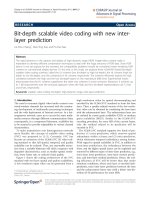
The LP structure proposed by Burt and Adelson [2] is shown
in Figure 1. For convenience of notation, let us consider an
LP for 1D signals; the results can b e carried over to the higher
dimensions in a straightforward manner with separable fil-

ters. For an image, for example, the filtering oper ations can
be performed first row-wise and then column-wise, each op-
eration using 1D signals. For the sake of explanation, we will
here consider an LP with only one level of decomposition.
For multiple levels of decompositions, the results can be de-
rived by repeating the operations on the lower-resolution
layer. Considering an input signal x of N samples and dyadic
downsampling, a coarse signal c can be derived as
1
c := Hx,(1)
where H denotes the decimation filter matrix of dimension
(N/2)
× N. H has the following general structure
2
:
H :
=
⎡
⎢
⎢
⎢
⎢
⎢
⎢
⎢
⎣
.
.
.
0 h(L) h(L

− 1) h(1) h(0) 0 0
00h(L) h(2) h(1) h(0)
.
.
.
⎤
⎥
⎥
⎥
⎥
⎥
⎥
⎥
⎦
.
(2)
The coefficients h(n), n
= 0, 1, 2, , L, here denote the
downsampling filter coefficients. The matrix structure above
is a result of the filtering (i.e., convolution) and downsam-
pling the filtered output by factor 2 (the elements of a row
are right-shifted by 2 columns from the elements of the pre-
vious row). We assume an FIR filter having linear phase
(i.e., symmetric). Repeated filtering and downsampling op-
erations on the coarsest signal leads to the so-called Gaus-
sian pyr amid. The first level of LP is obtained by predict-
ing the signal x based on the coarse signal c. The prediction
is made by upsampling the coarse signal with alternate zero
1
We use the no t a t i on “:=”for“isderivedas”or“isdefinedas.”

2
For a finite signal, because of the symmetric extension at the boundary,
the columns of H and G matrices at the left and at the right are flipped.
Wenxian Yang et al. 3
x
+
d
ol
−
p
ol
h
g
c
Q
d
Q
c
d
q
c
q
Figure 1: Open-loop Laplacian pyramid structure w ith one decom-
position level.
samples and then filtering the upsampled signal. In the SVC
framework, the LP coefficients need to be quantized before
being encoded. Depending on whether the quantizer for the
low-resolution signal is inside or outside the prediction loop,
there can be two different structures for the LP. The open-
loop prediction structure with the quantizer outside the loop

is shown in Figure 1. In this structure, the detail signal d
ol
is
given as
d
ol
:= x − Gc =

I
N
− GH

x,(3)
where I
N
denotes the identity matrix of order N and G de-
notes the interpolation filter matrix of dimension N
× (N/2).
G has the following general structure:
G:
=
⎡
⎢
⎢
⎢
⎢
⎢
⎢
⎢
⎣

.
.
.
0 g(0) g(1) g(2) g(M)0 0
00g(0) g(1) g(M
− 1) g(M)
.
.
.
⎤
⎥
⎥
⎥
⎥
⎥
⎥
⎥
⎦
t
.
(4)
The coefficients g(n), n
= 0, 1, 2, , M, here denote the up-
sampling filter coefficients and the superscript t denotes the
matrix transpose operation. Like the decimation filter ma-
trix, the interpolation filter matrix structure is a result of the
upsampling by factor 2 and filtering. The down-shifting of a
column by two rows from the previous column is due to the
alternate zero elements in the upsampled signal. The filter is
also assumed to be FIR and linear phase. Throughout the pa-

per, we assume normalized downsampling and upsampling
filters. That is,

n
h(n) = 1,

n
g(n) = 2. (5)
These normalization conditions guarantee that the coarse
signals and the prediction signals have about the same dy-
namic range as the original signal.
The closed-loop configuration with the quantizer within
the prediction loop is depicted in Figure 2. Here the quan-
tized coarse signal is used to make the prediction for the
x
+
d
cl
−
p
cl
h
g
c
Q
d
Q
c
d
q

c
q
Figure 2: Closed-loop Laplacian pyramid structure with one de-
composition level.
x
+
+
p
cl
g
d
q
c
q
Figure 3: Standard reconstruction structure for LP.
higher-resolution signal. If c
q
denotes the quantized low-
resolution sig nal, the detail signal is obtained as
d
cl
:= x − Gc
q
. (6)
Irrespective of the configuration, the coarse and the de-
tail signals are encoded with suitable transforms and variable
length coding (VLC) schemes before being transmitted to the
decoder. In Figures 1 and 2, we use the same symbols c
q
and

d
q
to denote the quantized coarse and detail signals. Clearly,
given the same quantizers, both structures transmit the same
coarse signal; however, the transmitted detail signals are dif-
ferent. We use the same symbol notation for the sake of sim-
plicity and also because of the fact that their usual recon-
struction structures (given in the next section) are identical.
In JSVM, the closed-loop prediction structure is adopted be-
cause of its superior performance compared to the open-loop
structure. Note that the coarse signal and the detail signals
here refer, respectively, to the base layer and the interlayer-
predicted enhancement layers in the JSVM.
3. LP DECODER STRUCTURES
The standard reconstruction method of an LP, either open-
loop or closed-loop, is shown in Figure 3. First the decoded
4 EURASIP Journal on Advances in Signal Processing
coarse signal is upsampled and then filtered using the same
interpolation filter as used at the encoder. This prediction
signal is added to the decoded detail signal to estimate the
original higher-resolution signal. Considering an LP with
only one level of decomposition, we can reconstruct the
original signal as
x
s
:= Gc
q
+ d
q
,(7)

where d
q
denotes the quantized or decoded detail signal. Ob-
serve that the prediction signal is identical to that for the
closed-loop LP encoder (when there are no channel errors).
Because of its overcompleteness, an LP can be repre-
sented as a fr ame expansion as follows. Let K denote the
resolution of the coarse signal c. For dyadic downsampling,
K
= N/2. The coarse and the detail signals can be jointly ex-
pressed as

c
d
ol

:=

H
I
N
− GH

x ≡ Sx,(8)
where S denotes the matrix on the right-hand side having
dimension (N + K)
× N. Since the LP is reversible for any
combinations of the downsampling and upsampling filters
h and g, S has full-column rank. The rows of S constitute a
frame and S can be called the frame operator or the analysis

operator associated with the LP [3, 9, 10].
The usual reconstruction shown in (7)canbeequiva-
lently expressed using the reconstruction operator [
GI
N
]as
x
s
:=

GI
N


c
q
d
q

. (9)
It is t rivial to prove that [
GI
N
]S = I
N
.In[3], Do and Vet-
terli propose to reconstruct the original signal using the dual
frame operator, which is (S
t
S)

−1
S
t
. It can be shown that if the
decimation and the interpolation filters are orthogonal, that
is, G
t
G = HH
t
= I
K
, G = H
t
, the dual frame operator cor-
responding to the frame operator in (8)is[
GI
N
− GH
][3].
If the filters are biorthogonal, that is, HG
= I
K
, the above
reconstruction operator is still an inverse operator (i.e., it is
a left-inverse of the analysis operator in (8)) even though it
is not the dual-frame operator [3]. Therefore, with either or-
thogonal or biorthogonal filters, the original signal can be
reconstructed as
x
f

:=

GI
N
− GH


c
q
d
q

=
G

c
q
− Hd
q

+ d
q
. (10)
The corresponding reconstruction structure is shown in
Figure 4. It is easy to see that the above dual frame based re-
construction is identical to the standard reconstruction when
the LP coefficients (both c and d
ol
) are not quantized.
The dual-frame-based reconstruction has the limitation

that the decimation and the interpolation filters need to be
at least biorthogonal. These filters, however, can lead to dis-
cernible and annoying aliasing in the coarse resolution signal.
The authors in [11 ] try to alleviate this problem by proposing
an update step at the encoder as shown in Figure 5(a).The
x
+
+
g
h
d
q
c
q
+
−
Figure 4: Frame-based reconstruction structure for LP.
detail signal d
ol
undergoes a low-pass filtering and downsam-
pling and this update signal is added to the coarse resolution
signal c as follows:
c
u
:= c + Fd
ol
, (11)
where F denotes the update filter matrix. The update filter
matrix has a similar structure as that of the decimation fil-
ter matr ix except that the filter coefficients h(n) are replaced

by the update filter coefficients f (n). The corresponding de-
coder, shown in Figure 5(b), has the same structure as the
frame-based reconstruction in Figure 4 except that the dec-
imation filter h is replaced by the update filter f. Thus, the
reconstructed signal is given as
x
u
:= G

c
uq
− Fd
q

+ d
q
= Gc
uq
+

I
N
− GF

d
q
, (12)
where c
uq
denotes the quantized updated coarse signal.

Obviously, when the decimation and the update filters
are identical, this reconstruction structure is the same as the
dual frame-based reconstruction. This lifted pyramid is re-
versible for any set of filters h, g,andf. In the special case,
when the decimation and the update filters are identical and
the decimation and the interpolation filters are biorthogonal,
the update signal is equal to zero, and hence this improved
pyramid is identical to the framed pyramid. Note that, like
the framed pyramid, this improved pyramid is also open-
loop. In the following, we propose some str u ctures for LPs
with nonbiorthogonal filters that are motivated from com-
pression point of view. As we show below, they can be applied
both in open-loop and closed-loop configurations.
4. IMPROVED OPEN-LOOP LP STRUCTURES
Consider first the open-loop configuration. When the up-
sampling and the downsampling filters are biorthogonal,
HG
= I
K
[3]. In this case, the detail signal obtained by
the standard prediction does not contain any low-frequency
component. This can be easily seen by downsampling the de-
tail signal
Hd
ol
= H

I
N
− GH


x = (H − HGH)x = 0
N/2×1
. (13)
Wenxian Yang et al. 5
x
+
d
ol
−
p
ol
h
g
f
c
Q
d
Q
c
d
q
c
uq
+
+
c
u
(a) Encoder
x

+
+
g
f
d
q
c
uq
+
−
(b) Decoder
Figure 5: Lifted-pyramid structure with an update step.
Therefore, the correlation between the coarse resolution sig-
nal c and the detail signal d
ol
is equal to zero.
Biorthogonality is a constrained relationship between the
downsampling and the upsampling filters: if the two fil-
ters are concatenated, the resulting filter is a half-band filter
which is symmetric about the frequency π/2[5, 12]. A sharp
roll-off of the decimation filter will require that the upsam-
pling filter has an overshoot close to the frequency π/2. This
has a negative impact on the compression efficiency of en-
hancement layers. Therefore, the filters used in the JSVM are
usually nonbiorthogonal. Throughout this paper, we assume
nonbiorthogonal downsampling and upsampling filters for
the LP as used in the JSVM.
Nonbiorthogonality, however, creates correlation be-
tween the low-resolution-coarse signal and the detail signal.
This can be seen from the following equation:

Hd
ol
= H

I
N
− GH

x =

I
K
− HG

Hx =

I
K
− HG

c.
(14)
Since HG
= I
K
, the right-hand side, in general, is nonzero.
The above equation can also be rewritten as
Hd
ol
=


I
K
− HG

c = c − Hp
ol
, (15)
where p
ol
denotes the open-loop prediction. This shows that
the low f requency component in the detail signal is equal to
the difference between the coarse signal and the downsam-
pled prediction signal. From compression point of view, this
correlation is an undesired feature since it leads to higher bit
rate.
4.1. Reduced-coarse signal
From (15), it is evident that the detail signal contains some
nonzero low-frequency component. This component can be
removed from the coarse signal since it can always be ex-
tracted from the detail signal at the receiver. Thus, we can
update the coarse signal as
c
r
:= c − Hd
ol
= c −

I
K

− HG

c = HGc = Hp
ol
, (16)
where c
r
denotes the reduced coarse signal. Thus, the reduced
coarse signal is equal to the filtered and downsampled pre-
diction signal. We term the new signal as reduced-coarse sig-
nal since the operation of upsampling followed by downsam-
pling can only lose information. The energy of the new coarse
signal relative to the original coarse signal, however, depends
on the signal itself, and can b e bounded by the squares of the
maximum and the minimum singular values of the operator
HG.
The updated coarse signal and the detail sig nal are quan-
tized at the desired bit rate and are transmitted. At the re-
ceiver, the decoder can estimate the coarse signal and the
original signal at higher resolution as
c := c
rq
+ Hd
q
,
x
c
:= Gc + d
q
= Gc

rq
+

I
N
+ GH

d
q
,
(17)
where c
rq
denotes the quantized reduced coarse signal. Ob-
serve that, to reconstruct the lower resolution coarse signal
c, the receiver needs to have received the higher resolution
detail signal d. Therefore, the above algorithm is not suitable
for SVC application. The alternative approach would be to
design the decimation and interpolation filters such that the
updated coarse signal c
r
, instead of c, has the desired low-
resolution quality. This approach does not require the avail-
ability of the detail signal to reconstruct the desired coarse
signal, which is c
r
. However, the filters need to be designed
differently from those used in the JSVM. Notice that this
method is similar to the open-loop LP structure of Flierl and
Vandergheynst [4] with the update filter equal to the down-

sampling filter and the addition (subtraction) operation at
the encoder (decoder) replaced by the subtraction (addi-
tion). They propose to follow the second approach through
the appropriate design of the three filters so that the equiva-
lent downsampling filter has the desired frequency response.
Therefore, in their approach, the low-resolution signal can be
reconstructed without the higher-resolution detail signal.
4.2. Reduced-detail signal
The second method to reduce the correlation is to keep the
low-resolution signal intact, but to remove the low-frequency
part from the detail signal. As we see in (15), this part could
be always computed by the decoder once it had received the
low resolution signal c. The encoder thus can update the
6 EURASIP Journal on Advances in Signal Processing
detail signal as
d
r
:= d
ol
− GHd
ol
=

I
N
− GH

d
ol
, (18)

where d
r
denotes the reduced detail signal. From the expres-
sion on the ri ght-hand side, we observe that the reduced de-
tail signal is nothing but the “detail of the detail,” that is, the
detail signal for the LP representation of the original detail
signal. We term the new detail as the reduced detail signal,
since the removal of the coarse component from the origi-
nal detail signal tends to reduce its energy. By substituting
the value of the low-frequency component from (15) and the
detail signal from (3), we get
d
r
= x − Gc − G

I
K
− HG

c = x −

2I
N
− GH

Gc. (19)
Thus, the updated detail signal can be obtained in one step
through an improved prediction which is given as
p
r

:=

2I
N
− GH

Gc =

2I
N
− GH

p
ol
. (20)
The coarse signal and the improved detail signal are
quantized at the desired bit rate and are transmitted. At the
receiver, the decoder first estimates the prediction and then
reconstructs the orig inal signal as
p
r
:=

2I
N
− GH

Gc
q
,

x
d
:= p
r
+ d
rq
=

2I
N
− GH

Gc
q
+ d
rq
,
(21)
where d
rq
denotes the quantized reduced detail signal. Note
that the correlation between the newly obtained detail sig-
nal and the coarse sig nal is still nonzero because of the non-
biorthogonality. However, it can be shown that the new cor-
relation is less than the original correlation. Since the detail
signal undergoes quantization after transform coding, and
the downsampling and upsampling operations increase the
complexity, we do not iterate the above operation further.
The above method has the advantage that it suits the
SVC application. We do not require the higher-resolution

enhancement layer signal to decode the low-resolution base
layer signal without redesigning the JSVM filters. However,
the above method stil l su ffers from the problem of the open-
loop, that is, the error at the higher resolution depends on
the quantization error of the coarse layer. In the following,
we present the above two methods in the closed-loop mode.
As we will see later, only the second method will lead to the
reconstruction error which is independent of the quantiza-
tion error of the coarse layer.
5. IMPROVED CLOSED-LOOP LP STRUCTURES
The purpose of the closed-loop prediction in the classical LP
structure is to avoid the mismatch between the predictions
at the encoder and at the decoder. This is achieved by in-
terpolating the quantized or decoded coarse resolution sig-
nal as the prediction. Since the predictions at the encoder
and the decoder are identical, the reconstruction error is
solely dependent on the quantization error of the detail sig-
nal. Further, this also implies that the reconstruction error is
bounded by the quantization step size of the detail layer. In
the following, we use the same notations as with the open-
loop configuration in order to avoid introducing further no-
tations, but their meanings should be clear from the consid-
ered configuration.
5.1. Reduced-coarse signal
In the closed-loop configuration, the encoder updates the
coarse signal based on the quantized detail signal. Thus, the
reduced detail signal is obtained as
c
r
:= c − Hd

q
. (22)
As in the open-loop configuration, the updated coarse sig-
nal is quantized at the desired bit rate and is transmitted. At
the receiver, the decoder estimates the coarse signal and the
original signal at higher resolution using (17). Observe that,
because of the quantized detail signal inside the update loop,
the update signal at the encoder and the decoder are identi-
cal. This update signal can be expressed as
Hd
q
= H

d
ol
+ q
d

=

I
K
− HG

c + Hq
d
, (23)
where q
d
represents the quantization noise of the detail sig-

nal. Here we have assumed an additive quantization noise
model. If the quantization noise is assumed to be highpass,
the second term on the right-hand side almost vanishes.
Therefore the update signal is almost the same as that in the
case of the open-loop configuration. As a consequence, there
will not be much difference in the reconstruction error com-
pared to that with the open-loop structure.
5.2. Reduced-detail signal
In the closed-loop configuration, the new prediction will be
based on the quantized- or decoded-coarse signal. Thus, the
new detail signal is obtained as
d
r
:= x −

2I
N
− GH

Gc
q
. (24)
The improved detail signal is quantized at the desired bit
rate and is transmitted. At the receiver, the decoder first com-
putes the prediction and then reconstructs the original signal
using (21). Because the decoder also uses the decoded-coarse
signal for prediction, there is no mismatch between the pre-
dictions made at the encoder and the decoder.
In the closed-loop prediction, the quality of the predic-
tion depends on the quantization parameter of the coarse

signal. If the quantization parameter is high, the detail sig-
nal can have larger energy, which implies higher bit rate. The
same is true for the proposed closed-loop structures.
Because of the compatibility with the SVC architecture,
here we will consider only the last method, that is, the closed-
loop improved prediction, for integration in the JSVM. The
two configurations with reduced-coarse signal can be incor-
porated in the SVC architecture provided the filters are de-
signed such that the reduced coarse signal has the desired
quality without aliasing. We will not address this problem
here since the filter design for SVC i s a separate problem.
Wenxian Yang et al. 7
6. RECONSTRUCTION ERROR ANALYSIS
Here we will assume that there is no channel noise, or e quiv-
alently all the channel errors have been successfully corrected
by forward error correction schemes. Thus, the reconstruc-
tion error at the receiver is solely due to the quantization
noise. In the following, we analyze the error performance of
the two methods in both the open-loop and the closed-loop
configurations.
6.1. Open-loop LP structures
As before, we will consider an LP with only one level of de-
composition. For the sake of simplicity of analysis, we will
assume that the coarse and the detail signals a re scalar quan-
tized. The quantization step sizes are small enough so that
the corresponding quantization noise components can be as-
sumed to be zero-mean, white, and uncorrelated. Further,
since in the open-loop the coarse signal and the detail signal
are quantized independently, their quantization noises can
be assumed to be uncorrelated.

6.1.1. LP with standard reconstruction
Let q
c
and q
d
denote the quantization noises for the coarse
signal and the detail signal, respectively. Assuming the quan-
tization noise to be additive, we can write
c
q
= c + q
c
, d
q
= d
ol
+ q
d
. (25)
Because of the afore-mentioned white-noise assumptions,
E

q
c
q
t
c

=
σ

2
c
I
K
, E

q
d
q
t
d

=
σ
2
d
I
N
, (26)
where σ
2
c
and σ
2
d
denote the variances of the coarse and the
detail signal components, respectively, and
E denotes the
mathematical expectation. Further, because of the assump-
tion of zero cross-correlation between the coarse signal and

the detail signal,
E

Gq
c
q
t
d

= E

q
d
q
t
c
G
t

=
0
N×N
. (27)
Referring to (7)and(3), the reconstruction error can be
expressed as
e
s
:= x
s
− x =


Gc
q
+ d
q

−

Gc + d
ol

= Gq
c
+ q
d
. (28)
Thus, the mean square error with the standard reconstruc-
tion is given as:
MSE
s
:=
1
N
E


e
s



2
=
1
N
E

e
t
s
e
s

=
1
N
E

Gq
c
+ q
d

t

Gq
c
+ q
d

=

1
N
σ
2
c
tr

G
t
G

+ σ
2
d
,
(29)
where the last expression follows from the assumptions
stated above. Here tr(
·) denotes the trace of the matrix. We
see that the reconstruction error is a function of the quan-
tization error of both the coarse signal and the detail signal.
Therefore, in a multiple-level LP, the reconstruction error at
any level contributes to the reconstruction error at all higher-
resolution levels. Observe that the reconstruction error i s also
a function of the upsampling filter matrix G. In practice, the
quantization noise of the coarse signal is dependent on the
coarse signal itself, and therefore, the reconstruction error
is also an indirect function of the downsampling filter ma-
trix H.
6.1.2. LP with frame reconstruction

Let q
cu
denote the quantization noise of the updated coarse
signal. Therefore, we can write c
uq
= c
u
+ q
cu
. Referring to
(12) for the frame reconstruction with an update, and using
(3)and(11), the reconstruction error can be expressed as
e
u
:= x
u
− x = Gq
cu
+

I
N
− GF

q
d
. (30)
Let us assume that q
cu
has similar statistical properties as that

of q
c
, that is, its components are white and uncorrelated with
variance σ
2
cu
, and they are uncorrelated with the components
of q
d
. Using similar steps as for the standard reconstruction,
the mean square error expression can be obtained as
MSE
u
:=
1
N
E


e
u


2
=
1
N
σ
2
cu

tr

G
t
G

+
1
N
σ
2
d
tr

I
N
− GF

t

I
N
− GF

.
(31)
In the special case when f (n)
= h(n), F = H, and therefore
MSE
u

=
1
N
σ
2
cu
tr

G
t
G

+
1
N
σ
2
d
tr

I
N
− GH

t

I
N
− GH


.
(32)
If the upsampling filter g(n) and the update filter f (n)turn
out to be biorthogonal, FG
= I
K
. In that case, the mean
square error can be simplified as
MSE
u
=
1
N
σ
2
cu
tr

G
t
G

+ σ
2
d

1 −
K
N


=
1
N
σ
2
cu
tr

G
t
G

+
σ
2
d
2
,(∵ K
= N/2).
(33)
6.1.3. Reduced-coarse signal
We will assume that the quantization noise of the reduced-
coarse signal has similar statistical properties as of the orig-
inal coarse signal. Even though the update signal depends
on the detail signal, for simplicity we will assume that the
quantization noise of the reduced coarse and the detail sig-
nals are uncorrelated. Let q
cr
denote the quantization noise
of the reduced-coarse signal. Therefore, c

rq
= c
r
+ q
cr
.Re-
ferring to (17), (3), and (16), the reconstruction error can be
expressed as
e
c
:= x
c
− x = Gq
cr
+

I
N
+ GH

q
d
. (34)
Thus, the mean square error can be derived as
MSE
c
:=
1
N
E



e
c


2
=
1
N
σ
2
cr
tr

G
t
G

+
1
N
σ
2
d
tr

I
N
+ GH


t

I
N
+ GH

,
(35)
where σ
2
cr
denotes the variance of the quantization noise q
cr
.
8 EURASIP Journal on Advances in Signal Processing
6.1.4. Reduced-detail signal
We will assume that the quantization noise of the reduced-
detail signal has similar statistical properties as of the original
detail signal. Further, the quantization noises of the coarse
and the detail signals c an be assumed to be uncorrelated. Let
q
dr
denote the quantization noise of the reduced detail signal.
Therefore, d
rq
= d
r
+ q
dr

. Referring to (21)and(19), the
reconstruction error can be expressed as
e
d
:= x
d
− x =

2I
N
− GH

Gq
c
+ q
dr
. (36)
Thus, the mean square error can be derived as
MSE
d
:=
1
N
E


e
d



2
=
1
N
σ
2
c
tr

G
t

2I
N
− GH

t

2I
N
− GH

G

+ σ
2
dr
,
(37)
where σ

2
dr
denotes the variance of the quantization noise q
dr
.
We observe that, for both structures, the reconstruction error
at any level of LP is dependent on the reconstruction errors
on the lower resolution layers.
6.2. Closed-loop LP structures
Let q
c
and q
d
denote the quantization noises for the coarse
signal and the detail signal, respectively. Assuming the quan-
tization noise to be additive, we can write
c
q
= c + q
c
, d
q
= d
cl
+ q
d
. (38)
We use the same notations for the errors and mean square
errors as in the open-loop configurations in order to avoid
introducing further symbols. We will further assume that the

quantization noises have similar statistical properties as in
the case of open-loop configurations.
6.2.1. LP with standard reconstruction
Referring to (7) for standard reconstruction, and using (6)
and (38), the reconstruction error can be expressed as
e
s
:= x
s
− x =

Gc
q
+ d
q

−

Gc
q
+ d
cl

=
q
d
. (39)
Thus, the mean square error with the standard reconstruc-
tion can be computed as follows:
MSE

s
:=
1
N
E


e
s


2
= σ
2
d
. (40)
We see that the reconstruction error is equal to the quantiza-
tion error of the detail signal. This is true even if we have an
LP with multiple layers.
6.2.2. Reduced coarse signal
Referring to (17), (3), and (22), the reconstruction error can
be expressed as
e
c
:= x
c
− x = Gq
cr
+ q
d

. (41)
Themeansquareerrorthuscanbederivedas
MSE
c
:=
1
N
E


e
c


2
=
1
N
σ
2
cr
tr

G
t
G

+ σ
2
d

. (42)
We see that the mean square error has a similar form to
that of the standard reconstruction in the open-loop struc-
ture. Since the aim of updating is to reduce the energy,
the encoding of the updated signal would have better rate-
distortion performance. This would imply effectively bet-
ter rate-distortion performance for the original signal at the
higher resolution. It is ev ident that, like the open-loop struc-
tures, the error is dependent on the quantization noise of the
lower-base layer.
6.2.3. Reduced-detail signal
Referring to (21)and(24), the reconstruction error can be
expressed as
e
d
:= x
d
− x = q
dr
. (43)
The error thus depends only on the quantization noise of the
reduced detail layer. The mean square error can be derived as
MSE
d
:=
1
N
E



e
d


2
= σ
2
dr
. (44)
The aim of the improved prediction is to reduce the en-
ergy of the detail signal. Following the results in information
theory [13], this would result in a better rate-distortion per-
formance for the encoding of the enhancement layer. This
implies that, for a given bit rate, the improved prediction
would result in less distortion. Comparing (40)and(44), this
would mean that σ
2
dr
<σ
2
d
.
7. TRANSFORM CODING OF ENHANCEMENT LAYER
In practice, the detail signal undergoes an orthogonal trans-
form before being quantized and entropy coded. The trans-
form aims to remove the spatial correlation in the detail sig-
nal coefficients and to compact its energy in fewer number
of coefficients. The current SVC standard, for this purpose,
uses a 4
× 4 integer transform, which is an approximation of

the discrete cosine transform (DCT) applied over a block size
of 4
× 4. The DCT, however, may not be the optimal trans-
form since the detail signal contains more high frequency
components. A closer look at (3) reveals that the detail sig-
nal has certain inherent structure. Most of its energy is con-
centrated along certain directions which are decided by the
downsampling and the upsampling filters. These directions
can be found out by the singular value decomposition [14 ]
of I
N
− GH as follows:
I
N
− GH ≡ UΣV
t
, (45)
where U and V are N
× N orthogonal matrices and Σ is
an N
× N diagonal matrix. In [15], we have shown that, in
open-loop configuration w ith biorthogonal upsampling and
downsampling filters, either the U matrix or the V matrix
applied on the detail signal leads to a critical representation
Wenxian Yang et al. 9
Video
Bitstream
Multiplex
2D spatial
decimation

Tem p or al
decomposition
Tex t ure
Intraprediction
for intrablock
Transfor m/
entr. coding
(SNR scalable)
Motion
Motion coding
2D spatial
interpolation
Improved
spatial
prediction
Core encoder
Motion
Decoded
frames
Tem p or al
decomposition
Tex t ure
Intraprediction
for intrablock
Transfor m/
entr. coding
(SNR scalable)
Motion
Motion coding
2D spatial

interpolation
Core encoder
Motion
Decoded
frames
Tem p or al
decomposition
Tex t ure
Intraprediction
for intrablock
Transfor m/
entr. coding
(SNR scalable)
Motion
Motion coding
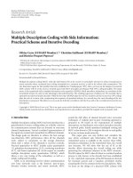
Core encoder
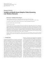
Figure 6: Improved scalable encoder using a multiscale pyramid with 3 levels of spatial scalability [1]. The proposed algorithm is embedded
in the “improved spatial prediction” module for the spatial intraprediction of the SD layer from the CIF layer for I and P frames.
of the LP. We refer to these matrices as the U-transform and
the V-transform, respectively. The 4
× 4 integer transform
applied in the JSVM is referred to as the DCT hereafter.
Under the closed-loop configuration, the above structure
is somewhat weakened. The introduction of the quantiza-
tion noise in the prediction loop destroys the redundancy
structure of the LP. Nevertheless, the above matrices are or-
thogonal and can always be applied to the original detail or
the newly-obtained detail signal. The decoder can use the
transpose of these matrices for the inverse transformation.
Experimental results presented in [15] showed that the V-

transform had a slightly better R-D performance than the
U-transform. Therefore, for the actual implementation with
JSVM, we consider only the V-transform.
8. IMPLEMENTATION WITH JSVM
Figure 6 depicts the structure of the improved JSVM en-
coder with the proposed spatial prediction module. The orig-
inal JSVM encoder is described in [1]. The encoder sup-
ports quality, temporal, and spatial scalabilities. A quality
base layer residual provides minimum reconstruction qual-
ity at each spatial layer. This quality base layer can be en-
coded into an AVC compliant stream if no interayer predic-
tion is applied. Quality enhancement layers are additionally
encoded and can be chosen to either provide coarse or fine
grain quality (SNR) scalability. To achieve temporal scalabil-
ity, hierarchical B pictures are employed. The concept of hi-
erarchical B pictures provides a fully predictive structure that
is already provided with AVC. Alternatively, motion compen-
sated temporal filtering (MCTF) can be used as a nonnorma-
tive encoder configuration for temporal scalability.
The encoder is based on a layered approach to achieve
spatial scalability. It provides a downsampling stage that gen-
erates the lower-resolution signals for lower layers. Each spa-
tial resolution (except the base layer, which is AVC coded)
includes refinement of the motion and texture information,
and the core encoder block for each layer basically consists
10 EURASIP Journal on Advances in Signal Processing
Table 1: Average number of MBs for mode selection over 8 intraframes for CITY SD at different QPs.
QP
Spatial intra
d d


QCIF/CIF SD DCT V-trans. DCT V-trans.
18,18
30 21.25 189.875 76.125 739.125 557.625
36 13.625 182.125 18.25 988.75 381.25
42 2.125 179.625 2.75 1289.875 109.625
48 0 176.375 0.625 1370.125 36.875
24,24
30 33.125 465.875 164.75 578.375 341.875
36 16 384.5 67.5 763 353
42 2 383 7.75 1075.375 115.875
48 0 384.375 0.25 1161.75 37.625
of an AVC encoder. T he spatial resolution hierarchy is highly
redundant. As shown in Figure 6, the redundancy between
adjacent spatial layers is exploited by different interlayer pre-
diction mechanisms for motion parameters as well as for tex-
ture data. For the texture data, the prediction mechanism
amounts to computing a difference signal between the orig-
inal higher-resolution signal and the interpolated version of
the coded and decoded signal at the lower-spatial resolution.
In our implementation, we aim to improve the coding
performance by exploiting the redundancy of the Laplacian
pyramid structure adopted for spatial scalability. To that end,
we modify only the interlayer texture prediction module
keeping the other modules same as in the original JSVM. Fur-
thermore, the or iginal downsampling and upsampling filters
are maintained. This means that the improved prediction in
(21) is obtained with the existing JSVM filters H and G.The
Fidelity Range Extension (FRExt) of SVC supports the high
profiles and adds more coding efficiency without a significant

amount of implementation complexity. The new features in
FRExt include an adaptive transform block-size and percep-
tual quantization scaling matrices. Our proposed method
also applies to FRExt, as will be discussed later. Through
theoretical analysis, improved interlayer motion and resid-
ual prediction can also be achieved, and this remains a future
work.
As we have mentioned earlier, in the current JSVM soft-
ware, the interlayer prediction is implemented in the closed-
loop mode. For each macroblock (MB), the selection of
prediction modes (interlayer, spatial-intra, temporal, etc.) is
based on a rate-distortion optimization (RDO) procedure.
However, the closed-loop structure does not guarantee an
improved rate-distortion performance either with the mod-
ified prediction or with the V-transform; the performance
can vary depending on the local signal statistics. Thus, to
apply the proposed method in SVC, we propose three ad-
ditional MB modes employing the improved prediction and
the V-transform besides the existing interlayer prediction
mode. The three proposed MB modes are (i) existing inter-
layer prediction followed by V-transform (d +V-transform),
(ii) improved prediction followed by DCT (d

+DCT),
(iii) improved prediction followed by V-transform (d

+V-
transform). We refer to the existing mode, interlayer predic-
tion followed by DCT, as “d + DCT.” The three proposed
modes are applied for encoding the SD layer by prediction

from the CIF layer.
The mode selec tion statistics over several frames are
shown in Ta ble 1 for intraframes. These statistics are ob-
tained by including all the modes in the original JSVM soft-
ware together with the three proposed modes and running
over 8 intraframes of the CITY video sequences. T he im-
proved prediction and the V-transform are applied only to
the SD layer while the QCIF and CIF layers are encoded us-
ing the existing modes. The table shows the number of mac-
roblocks undergoing different modes for different QP values
of QCIF, CIF, and SD layers. Note that the size of a mac-
roblock is 16
× 16 and the total number of macroblocks in
an SD image (with the resolution of 704
× 576) is equal to
1584. Thus, in Ta ble 1, the entries (number of macroblocks)
in each row add up to 1584.
From Tab le 1,firstweobservethatmajorityofmac-
roblocks choose the improved prediction irrespective of the
transform method followed, and especially at high QP values
of SD. This demonstrates that the proposed interlayer predic-
tion successfully reduces the redundancy and energy in the
detail signal.
Second, the number of blocks following the V-transform
is significant at low QPs of SD. However, the number of
blocks selecting the V-transform is always less than that
of blocks selecting the DCT. One reason is that the rate-
distortion in the current implementation is optimized w.r.t.
DCT. The rate-distortion optimization in mode selection
plays an important role to the overall coding performance.

In general video encoders, the mode that minimizes the cod-
ing cost, which is defined as
f
≡ R + λD, (46)
will be selected. Here R is the bitrate for coding the MB mode
syntax as well as the residual data and D is the corresponding
distortion. The optimal Lagrange multiplier λ should be se-
lected such that line f is tangent with the R-D curve, and is
defined as
λ
≡ 0.85 × 2
min(52,QP)/3−4
(47)
Wenxian Yang et al. 11
Table 2: Definition of macroblock modes for I and P frames in JSVM and proposed encoding scheme.
For I frames:
JSVM
Spatial-intra Intra 4 × 4, Intra 8 × 8
Interlay er texture (d +DCT) 4 × 4, (d +DCT) 8 × 8
Proposed Interla yer texture
(d +DCT)
4 × 4, (d +DCT) 8 × 8
(d + V-trans) 4 × 4, (d + V-trans) 8 × 8
(d

+DCT) 4 × 4, (d

+DCT) 8 × 8
(d


+ V-trans) 4 × 4, (d

+ V-trans) 8 × 8
For P frames:
JSVM
Spatial-intra Intra 4 × 4, Intra 8 × 8
Tem po ral
Skip, Inter
16 × 16, Inter 16 × 8,
Inter 8 × 16, Inter 8 × 8
Interlay er texture (d +DCT) 4 × 4, (d +DCT) 8 × 8
Interlayer MV/resi. IntraBLSkip, Inter 4, Inter 8, Inter 16
Proposed
Tem po ral
Skip, Inter
16 × 16, Inter 16 × 8,
Inter 8 × 16, Inter 8 × 8
Interlay er texture
(d +DCT)
4 × 4, (d +DCT) 8 × 8
(d + V-trans) 4 × 4, (d + V-trans) 8 × 8
(d

+DCT) 4 × 4, (d

+DCT) 8 × 8
(d

+ V-trans) 4 × 4, (d


+ V-trans) 8 × 8
Interlayer MV/resi. IntraBLSkip, Inter 4, Inter 8, Inter 16
empirically in the current JSVM implementation. However,
this λ is defined according to the DCT of the data to be en-
coded, and does not optimize the R-D performance of the
V-transform. Still we notice that the number of MBs select-
ing the V-transform is significant with lower QPs of the SD
layer. The improvement of applying the V-transform in our
proposed method remains a future work.
Overall, the proposed modes seem to be the chosen ones,
especially for low QP values of CIF and QCIF layers, that is,
better base layer qualities. It is also clear that the number of
MBs selecting the spatial intra mode is much smaller than
the number of MBs selecting the interlayer prediction modes.
Thus, we propose to suppress the spatial intra mode and
include the other three interlayer prediction modes. More
specifically, the MB modes used in original JSVM and the
proposed encoding scheme for I and P frames are defined as
in Table 2. Note that all the 8
× 8 modes are valid only when
FRExt is enabled.
Note that the V-transform is always applied over mac-
roblocks of size 16
× 16 for the luma component and of size
8
× 8 for the chroma components. Over a macroblock of size
16
× 16 (luma) or 8 × 8 (chroma), the order of complexity
is about the same as that of the existing 4
× 4transformex-

cept that the operations use floating-point numbers. In the
proposed modes adopting the V-transform, that is, d +V-
transform
4×4, d+V-transform 8×8, d

+V-transform 4×4,
d

+V-transform 8 × 8, the suffix(4× 4or8× 8) refers to the
block sizes for zigzag scanning of the transform coefficients.
Accordingly, the syntax for coding MB modes is also
modified. Two extra flags BLDetailFlag and BLTransformFlag
are needed in the syntax for signaling the additional MB
modes. BLDetailFlag defines whether the original spatial pre-
diction or the improved prediction is selected, a nd BLTrans-
formFlag selects between DCT a nd V-transform. These two
flags are encoded using the context adaptive binary arith-
metic coding (CABAC). Note that, since the spatial in-
tramode, which includes several submodes, is disabled, the
number of syntax bits of our proposed encoder remains sim-
ilar to that of the original JSVM.
The zigzag scanning, quantization, and entropy coding
methods of the transformed coefficients remain unchanged,
that is, those techniques as adopted in JSVM are also applied
to the transformed coefficients of the MBs selecting the pro-
posed modes. However, the quantizer in JSVM is designed to
be used in conjunction with the integer DCT transform, and
a multiplication factor MF is incorporated in the quantiza-
tion. To quantize the coefficients obtained by V-transform
directly, this multiplication factor is removed.

9. EXPERIMENTAL RESULTS AND ANALYSIS
The proposed scheme is tested using standard video se-
quences CITY and HARBOUR, and the anchor results are
obtained by JSVM 4.0. In the encoding of 3 spatial layers, that
is, QCIF, CIF, and SD, the proposed method is only applied
between the CIF layer and the SD layer. Thus, only the coding
12 EURASIP Journal on Advances in Signal Processing
29
30
31
32
33
34
35
36
37
PSNR (dB)
8 9 10 11 12 13 14 15
×10
3
Bitrate (kbps)
JSVM-18
Proposed-18
City SD, over 64 intraframes,
QP
= 18 for QCIF/CIF, luminance
(a) CITY, QP = 18
31
32
33

34
35
36
37
38
PSNR (dB)
10 10.51111.51212.51313.514
×10
3
Bitrate (kbps)
JSVM-18
Proposed-18
Harbour SD, over 64 intraframes,
QP
= 18 for QCIF/CIF, luminance
(b) HARBOUR, QP = 18
27
28
29
30
31
32
33
34
35
36
37
PSNR (dB)
4 5 6 7 8 9 10 11 12
×10

3
Bitrate (kbps)
JSVM-24
Proposed-24
City SD, over 64 intraframes,
QP
= 24 for QCIF/CIF, luminance
(c) CITY, QP = 24
30
31
32
33
34
35
36
37
PSNR (dB)
66.577.588.599.51010.511
×10
3
Bitrate (kbps)
JSVM-24
Proposed-24
Harbour SD, over 64 intraframes,
QP
= 24 for QCIF/CIF, luminance
(d) HARBOUR, QP = 24
27
28
29

30
31
32
33
34
35
36
PSNR (dB)
234567891011
×10
3
Bitrate (kbps)
JSVM-30
Proposed-30
City SD, over 64 intraframes,
QP
= 30 for QCIF/CIF, luminance
(e) CITY, QP = 30
29
30
31
32
33
34
35
36
37
PSNR (dB)
345678910
×10

3
Bitrate (kbps)
JSVM-30
Proposed-30
Harbour SD, over 64 intraframes,
QP
= 30 for QCIF/CIF, luminance
(f) HARBOUR, QP = 30
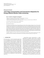
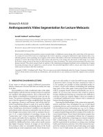
Figure 7: PSNR-rate curves for the luminance component of (a) CITY and (b) HARBOUR SD 30 Hz over 64 intraframes, when QPs for
QCIF/CIF are 18, 24, 30.
Wenxian Yang et al. 13
27
28
29
30
31
32
33
34
35
36
PSNR (dB)
44.555.56 6.5
×10
3
Bitrate (kbps)
JSVM-18
Proposed-18
City SD, o v er 64 IP frames,
QP

= 18 for QCIF/CIF, luminance
(a) CITY, QP = 18
28
29
30
31
32
33
34
35
36
37
PSNR (dB)
6 7 8 9 10 11 12 13 14 15
×10
3
Bitrate (kbps)
JSVM-18
Proposed-18
Harbour SD, over 64 IP frames,
QP
= 18 for QCIF/CIF, luminance
(b) HARBOUR, QP = 18
27
28
29
30
31
32
33

34
35
36
PSNR (dB)
1.522.533.544.5
×10
3
Bitrate (kbps)
JSVM-24
Proposed-24
City SD, o v er 64 IP frames,
QP
= 24 for QCIF/CIF, luminance
(c) CITY, QP = 24
28
29
30
31
32
33
34
35
36
PSNR (dB)
33.544.555.566.5
×10
3
Bitrate (kbps)
JSVM-24
Proposed-24

Harbour SD, over 64 IP frames,
QP
= 24 for QCIF/CIF, luminance
(d) HARBOUR, QP = 24
27
28
29
30
31
32
33
34
35
36
PSNR (dB)
0.511.522.533.5
×10
3
Bitrate (kbps)
JSVM-30
Proposed-30
City SD, o v er 64 IP frames,
QP
= 30 for QCIF/CIF, luminance
(e) CITY, QP = 30
28
29
30
31
32

33
34
35
36
PSNR (dB)
11.522.533.544.555.56
×10
3
Bitrate (kbps)
JSVM-30
Proposed-30
Harbour SD, over 64 IP frames,
QP
= 30 for QCIF/CIF, luminance
(f) HARBOUR, QP = 30
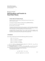
Figure 8: PSNR-rate curves for the luminance component of (a) CITY and (b) HARBOUR SD 30 Hz over 64 I and P frames, with GOP
size
= 1 and Intraperiod = 8, when QPs for QCIF/CIF are 18, 24, 30.
14 EURASIP Journal on Advances in Signal Processing
results of the SD layer are presented. Since FGS layers are not
involved in our experiments, we set both QPs for QCIF/CIF
to 18, 24, and 30, w hich approximately correspond to the
base-layer quality with the initial QP 36, 42, and 48 plus three
FGS layers. First we test the proposed method using 64 in-
traframes. Then we test the proposed method using the GOP
structure defined as GOPSize
= 1 and IntraP eriod = 8,which
means one I frame fol lowed by 7 P frames for every 8 frames.
Other parameters in the configuration files are listed as fol-
lows:FRExt:off for QCIF layer, on for CIF/SD layers; Loop

Filter: on; Update Step: 0; Adaptive QP: 1; Inter Layer Pred:
0 for QCIF layer, 2 for CIF/SD layers; Number of FGS layers:
0. Results for all Intraframes are shown in Figure 7, and the
results with P frames are shown in Figure 8. We observe that
the proposed improved prediction works well for small QP
values for CIF/QCIF layers. As the QP is increased, the pre-
dictionbecomeslessefficient. With QP equal to 18, PSNR
gain up to 1 dB can be achieved with all intraframes and a
gain up to 0.7 dB gain can be achieved with Intra and inter P
frames (with HARBOUR sequence).
We must note here that, for all the simulations, we did
not modify the entropy coding that follows the transform
(DCT or V-transform). In the current JSVM software, it
is implemented as context adaptive variable length coding
(CAVLC). The current zigzag scan and the coding scheme
are optimized for the DCT; therefore, we expect better re-
sults if the scanning and encoding of the V-transformed co-
efficients are modified so as to suit the characteristic of the
V-transform. This is a subject of research and we will not
pursue it in this paper.
10. CONCLUSIONS
In this paper, we have proposed two improved Laplacian
pyramid structures for scalable video coding. The proposed
structures exploited the inherent redundancy of the underly-
ing Laplacian pyramid with nonbiorthogonal filters by ren-
dering the enhancement-layer signal less correlated with the
base-layer. The first structure updated the base-layer sig-
nal by subtracting from it the low-frequency component of
the enhancement-layer signal. The second st ructure modi-
fied the prediction with a view to reducing the low-frequency

component in the enhancement layer. The corresponding de-
coder structures were accordingly modified in order to re-
construct the signal at both resolution levels. The simplic-
ity of the structures is reflected by the fact that they did
not require to modify the current upsampling filter, nor did
they require to design additional filters. Moreover, the struc-
tures could be implemented both in the open-loop and in the
closed-loop configurations.
We studied the distortion performances of both struc-
tures in the open-loop and in the closed-loop configurations.
Open-loop structures used unquantized continuous-valued
update signals whereas the closed-loop signals used the de-
coded quantized signals for the purpose. It was demonstrated
that only the second structure (with reduced enhancement
layer) in the closed-loop configuration leads to a reconstruc-
tion error that is dependent on the quantization error of the
enhancement layer, but not on the reconstruction error of
the lower-resolution layers. Out of the two structures, it was
also the only structure that w as compatible with the current
JSVM architecture.
Along with a recently proposed transform for the en-
hancement layer, the proposed structure was integrated with
JSVM in the SD layer. Based on the experimental results,
the macroblock modes in I and P frames were redesigned.
Results with test sequences demonstrated that the proposed
scheme achieves better R-D performance compared to the
original prediction modes. The performance improvement
was significant in the case of low-base layer QP suggesting
potential application of the proposed method in high-quality
scalable video coding.

For the present JSVM integration, there are still some
open issues such as the optimization of the VLC for the V-
transform, the choice of the λ para meter in rate-distortion
optimized mode selection, the optimization of the FGS,
and so forth. Further research results along these directions
can provide us the complete picture on the true coding
performance of the proposed method. Experimental results
demonstrate that interlayer prediction is the dominant mode
in I frames, and the stationary regions in P and B fr ames.
Thus, the proposed method could have a significant impact
on the overall coding performance of still sequences or se-
quences having low-motion level.
REFERENCES
[1] JVT, “Joint scalable video model JSVM-4,” in Joint Video
Team (JVT) of ISO/IEC MPEG & ITU-T VCEG (ISO/IEC
JTC1/SC29/WG11 and ITU-T SG16 Q.6), Nice, France, Octo-
ber 2005.
[2] P. J. Burt and E. H. Adelson, “ The Lapacian pyramid as a
compact image code,” IEEE Transactions on Communications,
vol. 31, no. 4, pp. 532–540, 1983.
[3] M. N. Do and M. Vetterli, “Framing pyramids,” IEEE Transac-
tions on Signal Processing, vol. 51, no. 9, pp. 2329–2342, 2003.
[4] M. Flierl and P. Vandergheynst, “An improved pyramid for
spatially scalable video coding,” in Proceedings of IEEE Inter-
national Conference on Image Processing (ICIP ’05), vol. 2, pp.
878–881, Genova, Italy, September 2005.
[5] D. Santa-Cruz, J. Reichel, and F. Ziliani, “Opening the Lapla-
cian pyramid for video coding,” in Proceedings of IEEE Inter-
national Conference on Image Processing (ICIP ’05), vol. 3, pp.
672–675, Genova, Italy, September 2005.

[6] A. Segall, “Study of upsampling/down-sampling for spatial
scalability,” in Joint Video Team (JVT) of ISO/IEC MPEG &
ITU-T VCEG (ISO/IEC JTC1/SC29/WG11 and ITU-T SG16
Q.6), Nice, France, October 2005.
[7] A. Segall, “Upsampling and down-sampling for spatial scala-
bility,” in Joint Video Team (JVT) of ISO/IEC MPEG & ITU-
T VCEG (ISO/IEC JTC1/SC29/WG11 and ITU-T SG16 Q.6),
Bangkok, Thailand, January 2006.
[8] C. K. Kim, D. Y. Suh, and G. H. Park, “Directional filtering
for upsampling according to direction information of the spa-
tially lower layer,” in Joint Video Team (JVT) of ISO/IEC MPEG
& ITU-T VCEG (ISO/IEC JTC1/SC29/WG11 and ITU-T SG16
Q.6), Bangkok, Thailand, January 2006.
Wenxian Yang et al. 15
[9] V.K.Goyal,J.Kova
ˇ
cevi
´
c, and J. A. Kelner, “Quantized frame
expansions with erasures,” Applied and Computational Har-
monic Analysis, vol. 10, no. 3, pp. 203–233, 2001.
[10] I. Daubechies, Ten Lectures on Wavelets, SIAM, Philadelphia,
Pa, USA, 1992.
[11] M. Flierl and P. Vandergheynst, “Inter-resolution transform
for spatially scalable video coding,” in Proceedings of Picture
Coding Symposium (PCS ’04), pp. 243–247, San Francisco,
Calif, USA, December 2004.
[12] P. P. Vaidyanathan, Multirate Systems and Filter Banks,
Prentice-Hall, Englewood Cliffs, NJ, USA, 1993.
[13] T. M. Cover and J. A. Thomas, Elements of Information Theory,

Wiley-Interscience, New York, NY, USA, 1991.
[14] G. Strang, Linear Algebra and Its Applications, Brooks Cole
Publishers, Florence, Ky, USA, 3rd edition, 1988.
[15] G. Rath and C. Guillemot, “Compressing the Laplacian pyra-
mid,” in Proceedings of the 8th IEEE Workshop on Multime-
dia Signal Processing (MMSP ’06), pp. 75–79, Victoria, BC,
Canada, October 2006.
Wenxian Yang received the B.Eng. degree
from Zhejiang University, Hangzhou,
China, in 2001 and the Ph.D. degree in
Computer Engineering from Nanyang
Technological University, Singapore, in
2006. In 2004, she was with Microsoft Re-
search Asia, Beijing, China for internship.
From 2005 to 2006, she was a Postdoctoral
Researcher in the French National Institute
for Research in Computer Science and
Control (INRIA-IRISA), France. She is now a Postdoctoral Fellow
in The Chinese University of Hong Kong. Her research interests
include video compression, 3D video compression and processing.
Gagan Rath received the B.Tech. degree in
electronics and electrical communication
engineering from the Indian Institute of
Technology at Kharagpur in 1990 and the
M.E. and Ph.D. degrees in electrical com-
munication engineering from the Indian
Institute of Science in Bangalore in 1993
and 1999. He is currently a Research Scien-
tist at INRIA in France. His research inter-
ests include signal processing for communi-

cations, distributed video coding, scalable video coding, and joint
source and channel coding.
Christine Guillemot is currently Directeur
de Recherche at INRIA, in charge of the
TEMICS research group dealing with im-
age modelling, processing, video commu-
nication, and watermarking. She holds the
Ph.D. deg ree from Ecole Nationale Su-
perieure des Telecommunications (ENST)
Paris. From 1985 to October 1997, she has
been with FRANCE TELECOM/CNET,
where she has been involved in various
projects in the domain of coding for TV, HDTV and multi-
media applications, and coordinated a few (e.g., the European
RACE-HAMLET project). From January 1990 to mid 1991, she
has worked at Bellcore, NJ, USA, as a visiting scientist. Her re-
search interests are signal and image processing, video coding,
and joint source and channel coding for video transmission over
the Internet and over wireless networks. She has served as Associate
Editor for IEEE Trans. on Image Processing (2000–2003), and for
IEEE Trans. on Circuits and Systems for Video Technology (2004–
2006). She is a member of the IEEE IMDSP and of the IEEE MMSP
technical committees.