Báo cáo hóa học: " Research Article A Time-Domain Fingerprint for BOC(m, n) Signals" doc

Hindawi Publishing Corporation
EURASIP Journal on Advances in Signal Processing
Volume 2007, Article ID 56104, 7 pages
doi:10.1155/2007/56104
Research Article
A Time-Domain Fingerprint for BOC(m, n) Signals
B. Muth,
1
P. Oonincx,
1
and C. Tiberius
2
1
Faculty of Military Sciences, Netherlands De f ence Academy, Het Nieuwe Diep 8, 1781 AC Den Helder, The Netherlands
2
Department of Earth Observation and Space Systems (DEOS), Delft University of Technology, Kluyverweg 1,
2629 HS Delft, The Netherlands
Received 3 November 2006; Accepted 10 April 2007
Recommended by Sudharman Jayaweera
Binary offset carrier (BOC) describes a class of spread-spectrum modulations recently introduced for the next generation of global
navigation satellite systems (GNSSs). The design strategies of these BOC signals have so far focused on the spectral properties of
these signals. In this paper, we present a time-domain fingerprint for each BOC signal given by a unique histogram of counted
time elapses between phase jumps in the signal. This feature can be used for classification and identification of BOC-modulated
signals with unknown parameters.
Copyright © 2007 B. Muth et al. This is an open access article distributed under the Creative Commons Attribution License, which
permits unrestricted use, distribution, and reproduction in any medium, provided the original work is properly cited.
1. INTRODUCTION
In the scope of emerging radionavigation satellite systems,
the binary offset carrier (BOC) modulation is of special
interest. The new generation of global navigation satellite
systems (GNSSs), modernized GPS [1], and the European

Galileo system [2] will use BOC (or BOC-based) signals on
different carriers and with different parameters, to enable
ranging. The main reasons for creating BOC signals were,
on one hand, the need to improve traditional GNSSs sig-
nals properties for better resistance to multipath interfer-
ences of all kinds and receiver noise [3, 4], and on the other
hand, the need for improved spectral sharing of the allo-
cated bandwidth with existing signals or future signals of
the same class [3, 5]. Particularly, correlation and spectral
properties were improved during the BOC design process.
The improvements for the acquisition and tracking of fu-
ture GNSSs signals have been assessed and new algorithms
have been elaborated. We study the behaviour of BOC sig-
nals from a different point of view, namely, by counting and
accumulating time elapses between phase jumps in the sig-
nal.
The paper is organised as follows. After introducing
BOC(m, n) signals in Section 2, we study the statistical be-
haviour of the length of time intervals between phase jumps
in BOC(m, n) signals in Sections 3 and 4. We refer to these
time intervals as run lengths and will not focus on their
computation. Studying these run lengths will be based upon
arithmetic relationships between the BOC parameters m
and n, using some elementary combinatorial relations. In
Section 5, convergence results for the obtained statistics are
derived as a function of the number of measured code chips.
Furthermore, we present examples of distributions of run
lengths derived for specific parameters m and n to illustrate
the results. Finally, some conclusions and directions for fur-
ther research are presented in Section 6. In this perspective,

we also briefly discuss related signal structures, like MBOC
and cosine-phased BOC.
2. BINARY OFFSET CARRIER SIGNAL
A BOC-modulated signal consists of a sinusoidal carrier, a
subcarrier, a pseudorandom noise (PRN) spreading code,
and a data sequence. The BOC signal is the product in the
time domain of these components. To investigate the appear-
ances of singularities (jumps) in a BOC signal we focus on
the product of the subcarrier waveform and the spreading
code sequence. Since the sinusoidal carrier is continuous and
thus does not contribute to any phase jump in the modulated
signal, we do not take the behaviour of this carrier wave into
account in the sequel of this paper. Furthermore, the data se-
quence is not taken into account, since it usually has a far
lower frequency than all other components [6].
To introduce BOC signals, we take 2T
s
(resp., f
s
) as the
subcarrier period (resp., frequency). For the subcarrier sev-
eral waveforms are possible. In this paper, we will limit our
study to the case of a rectangular sine-phased subcarrier. Be-
sides, we will refer to the spreading symbols (resp., sequence)
2 EURASIP Journal on Advances in Signal Processing
in the code as pseudo-random noise (PRN) chips (resp.,
code). The length (resp. chipping rate or code rate) of such a
PRN chip is denoted by T
c
(resp., f

c
). Physically, that means
that the code might change (but not necessarily) from
−1
to +1 and conversely every 1/f
c
second. In addition, we as-
sume that the spreading code is a sequence of independent
and identically distributed random variables. As a result, we
do not take into account any additional requirements on the
correlation function of the spreading code, for example, see
[7]. The reason for doing this is that in our study we only
consider a limited number of code chips, while the mathe-
matical requirements on the code can only be verified when
considering the whole code, containing much more code
chips.
GNSSs satellites have an atomic clock on-board with a
nominal reference frequency f
0
from which all c omponents
of the generated navigation signals are derived. In case of a
BOC signal, besides the carrier frequency also the subcarrier
frequency f
s
and the code rate f
c
are multiples of f
0
, that is,
f

s
= m · f
0
, f
c
= n · f
0
. The BOC signal with subcarrier fre-
quency mf
0
and code rate nf
0
is referred to as BOC(m, n).
For the sake of simplicity, m and n are assumed to be positive
integers, with m
≥ n, w hich is the case in practice. Signals
like BOC(15, 2.5) also appear in literature. Such type of sig-
nals is intended for specific services such as the galileo public
regulated service (PRS) to be of interest for experts. As we
will see in the next section only the division of m by n is of
importance for the results in this paper, not the values of m
and n themselves.
Although in this paper we will only concentrate on the
code subcarrier product within a BOC signal, here we briefly
mention the formal time and frequency representation of
a BOC signal. The complex envelope representation of the
BOC signal is given by
s(t)
= exp(−iθ)


j
a
j
· μ
kT
s

t − jkT
s
− t
0

·
c
T
s

t − t
0

,
(1)
with a
j
the sequence of data-modulated spreading code val-
ues, μ
kT
s
(t) the spreading symbol of duration T
c

= kT
s
, c
T
s
(t)
the subcarrier of period 2T
s
and k the number of subcarrier
half-periods during which the spreading code value remains
unchanged. The frequency spectrum of a BOC( f
s
, f
c
) signal
reads for k,even,
G( f )
=
1
kT
s

sin

πfT
s

sin

kπ f T

s

πf cos

kπ f T
s


2
= f
c

tan

πf/2 f
s

sin

πf/f
c

πf

2
.
(2)
Whereas for k odd, we have
G( f )
=

1
kT
s

sin

πfT
s

cos

kπ f T
s

πf cos

kπ f T
s


2
= f
c

tan

πf/2 f
s

cos


πf/f
c

πf

2
.
(3)
For the derivation of the BOC spectrum we refer to [3].
Code sequence: ±[1, 1]
1
0
−1
0 T
s
2T
s
3T
s
4T
s
Subcarrier
Code sequence: ±[1, −1]
1
0
−1
0 T
s
2T

s
3T
s
4T
s
1
0
−1
0 T
s
2T
s
3T
s
4T
s
PRN code
1
0
−1
0 T
s
2T
s
3T
s
4T
s
1
0

−1
0 T
s
2T
s
3T
s
4T
s
Product
1
0
−1
0 T
s
2T
s
3T
s
4T
s
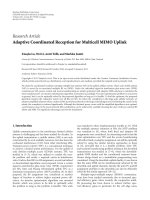
Figure 1: Product of BOC(1, 1) subcarrier and spreading code for
two code possibilities.
3. RUN LENGTH HISTOGRAMS FOR BOC(kn/2, n)
The time-domain fingerprint for BOC signals we introduce
in this paper is based on the time elapses between consecu-
tive phase jumps in a BOC signal. These phase jumps are due
to jumps (discontinuities) in the code subcarrier product. In
Figure 1, five of such jumps are shown in the left-hand ex-
ample and four of such transitions show up in the right-hand

example. The time elapses between these jumps (T
s
at the left
and T
s
and 2T
s
at the right) are referred to as run lengths.
As a starting point for studying run length appearing
in BOC(m, n) signals is to consider the class BOC(m,1),
m
= 1, 2, 3, Results for BOC(kn/2, n), with integer k,
are obtained straightforwardly from this BOC(m,1) case.
Moreover, a n extension of the method used for deducing the
BOC(m, 1) results will be used in the next section for yield-
ing results on the run lengths for general BOC(m, n) signals,
with m
≥ n.
We will first concentrate on BOC(m, 1) as a special case
of BOC(kn/2, n)withk
= 2m, n = 1. For BOC(m, 1) signals,
we consider sections of length pT
c
containing exactly p PRN
chips. Since T
c
= mT
s
, pm half periods of the subcarrier may
appear during such a section. Here a half period is considered

as an interval of half the length of the subcarrier’s period,
that is also marked by a parity jump in the code subcarrier
product. We identify one half period with its length T
s
.
The number of half periods appearing in the combined
BOC signal dur ing p PRN chips also depends on the spread-
ing code. If a code is changing state, then the product of code
and subcarrier will not change its state at that particular mo-
ment in time, yielding an extension of that spreading-code
half period to a full period. Then the number of half peri-
ods T
s
, indicated by N(T
s
), is divided by a factor 2 and the
number of full periods 2T
s
,givenbyN(2T
s
), increases by 1.
We observe, that for BOC(m, 1), only full and half periods
can appear like this, since the state jumps of the chips always
coincide with jumps of the subcarr i er.
B. Muth et al. 3
Table 1: BOC(m, 1) run length counts for all possible code subcarrier combinations.
Number of PRN chips p Number of half periods T
s
Number of periods 2T
s

Number of code possibilities Code possibilities
2
4m (2
· 2m) 0 1 [1, 1]
4m
− 2(2· 2m − 2) 1 1 [1, −1]
3
6m (3
· 2m) 0 1 [1, 1, 1]
6m
− 2(3· 2m − 2) 1 2
[1, 1,
−1]
[
−1, 1, 1]
6m
− 4(3· 2m − 4) 2 1 [1, −1, 1]
4
8m (4
· 2m) 0 1 [1, 1, 1, 1]
8m
− 2(4· 2m − 2) 1 3
[
−1, 1, 1, 1]
[1, 1,
−1, −1]
[1, 1, 1,
−1]
8m
− 4(4· 2m − 4) 2 3

[
−1, 1, 1, 1]
[
−1, 1, 1, 1]
[
−1, 1, 1, 1]
8m
− 6(4· 2m − 6) 3 1 [1, −1, 1, −1]
To illustrate these considerations we take as an example
BOC(1, 1) during p
= 2 PRN chips as depicted in Figure 1.
Two possible situations can appear. First, in case the PRN se-
quence is
±[1, 1], the product of code and subcarrier con-
tains 4 run lengths of duration T
s
(left graph). Second, in
case the PRN s equence is
±[1, −1], the second and third half
periods have the same state and are therefore merged to one
full periods time inter val. So, in this case, the product of code
and subcarrier contains 2 r un lengths of duration T
s
and 1 of
duration 2T
s
(right graph).
We can follow the same observations for BOC(m,1)sig-
nals for p
= 2, 3, 4. The appearances of half and full peri-

ods (T
s
versus 2T
s
) between parity changes in the code sub-
carrier product have been counted for all possible combi-
nations of code and subcarrier. The results can be found in
Table 1. There the second and third columns show the num-
ber of half and full periods that can appear in one code sub-
carrier product within a duration of p code chips. In the
fourth column, the number of different code combinations
that can appear in the various situations is indicated.
What can be observed from Ta bl e 1 is that, for N(T
s
),
multiples of 2 are subtracted from 2pm,eachtimeN(2T
s
)
is increased by 1. Also we note that the number of possible
codes follows binomial coefficients. In fact, these numbers
should be multiplied by 2, since all codes also have a counter-
part (multiply code by
−1). However, for our computations,
we identify the counterparts with the original codes.
Extrapolating the observations of Tab le 1 for higher val-
ues of p, we derive expressions for the expected values of
N(T
s
)andN(2T
s

). This is done by accumulating all 2
p−1
pos-
sible combinations and taking the mean, that is,
N

T
s

=
2
1− p
p
−1

k=0

p − 1
k

(2pm − 2k),
N

2T
s

=
2
1− p
p

−1

k=0

p − 1
k

k.
(4)
Using a corollary of Newton’s binomial theorem, (4)can
be rewritten as
N

T
s

= 2
1−p

2pm · 2
p−1
−2(p− 1) · 2
p−2

= 2pm− p+1,
(5)
N

2T
s


= 2
1− p
· (p − 1)2
p−2
=
p − 1
2
. (6)
For large p, a distribution of the two types of run lengths
in BOC(m, 1) is obtained by taking
lim
p→∞
N

T
s

N

2T
s

=
lim
p→∞
4pm − 2p +2
p − 1
= 4m − 2. (7)
This means that for reasonable large p afractionof1/(4m

−1)
of all intervals between phase jumps in BOC(m,1) is of
length 2T
s
,and(4m − 2)/(4m − 1) of those inter vals are of
length T
s
. Typically for BOC(1, 1) we have an expected dis-
tribution of 1/3versus2/3.
An extension of the previous results yields the distribu-
tion of run lengths for signals of type BOC(kn/2, n), since
for these signals the characteristics and construction of the
code subcarrier product coincide with those of BOC(k,2)
up to a division/multiplication of T
c
and T
s
by n.Asare-
sult for BOC(kn/2, n), we have the same run length statistics
as for BOC(k/2, 1). More general, i n the case of BOC(m, n)
with n a divisor of 2m, the distribution of length 2T
s
in-
tervals versus length T
s
intervals in the signal is given by
1/(4m/n
− 1) = n/(4m − n)versus(4m/n − 2)/(4m/n − 1) =
(4m − 2n)/(4m − n). As a special case we have the distribu-
tion 1/3versus2/3forallBOC(m, m).

4. RUN LENGTH RESULTS FOR ARBITRARY BOC(m, n)
One may easily verify that all types of BOC(m, n) signals dis-
cussed in the previous section satisfy gcd(2m, n)
= n (great-
est common divisor). Here we discuss all other possibilities,
namely, 1
≤ gcd(2m, n) <n, starting with gcd(2m, n) = 1,
4 EURASIP Journal on Advances in Signal Processing
Code: [−1, 1, 1, −1, 1, 1]
1
0
−1
Subcarrier
1
0
−1
PRN code
1
0
−1
Product
Time
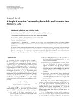
Figure 2: Components of a BOC(5, 3) signal i n the time-domain.
The vertical solid indicators displayed over the code correspond to
the subcarrier phase jumps, whereas the dashed indicators in the
PRN code correspond to the possible transitions in the code state.
The ellipse illustrates the first observation made in this section,
namely, the coincidence of the nth possible code change with the
2mth subcarrier state change.
that is, 2m and n are relatively prime. Translated in terms of

the code subcarrier product we observe that
(i) Every nth possible code change coincides with every
2mth phase jump in the subcarrier;
(ii) Between such coinciding phase jumps, n
− 1 possible
code changes do not coincide with subcarrier jumps,
but intersect 2m subcarrier half periods.
These observations have been depicted for BOC(5, 3) in
Figure 2.
The run length statistics can be obtained by construction,
with respect to these two observations. Considering only the
first observation, we would have the same run length statis-
tics as for BOC(m, 1). The second observation introduces the
possibility of having n
− 1 other run length values (i/n)T
s
,
i
= 1, 2, , n − 1 by intersection, that all may appear twice
within n chips. This double counting is due to the fact that a
code change first yields a run length contribution of (i/n)T
s
and ((n − i)/n)T
s
, and at a later stage may contribute with
lengths of ((n
− i)/n)T
s
and (i/n)T
s

. The construction of this
BOC(m, n) run length distribution with gcd(2m, n)
= 1is
also illustr ated in Figure 4. We start from the steady distribu-
tion for BOC(m,1), given by N(T
s
):N(2T
s
) = 4m − 2:
1 (see Figure 3). Next, m
− 1 intervals of length T
s
may
be divided into two smaller intervals of length kT
s
/n and
(n
− k)T
s
/n. Concluding, for this type of BOC(m, n), we ob-
tain the relation
N

T
s
/n

.
.
. N


2T
s
/n

.
.
.
···
.
.
. N

(n−1)T
s
/n

.
.
. N

T
s

.
.
. N

2T
s


2
.
.
.2
.
.
.
···
.
.
.2
.
.
.4m
−2−(n − 1)
.
.
.1
(8)
or equivalently, for large p, a fraction of 1/(4m + n
− 2) of all
intervals between phase jumps in BOC(m, n)isoflength2T
s
,
BOC(m,1) BOC(m, n)
N(T
s
) ∼ 4m − 2 N(T
s

) ∼ 4m − 2 − (n − 1)
N(T
s
/n) ∼ 2
N(2T
s
/n) ∼ 2
.
.
.
N((n
− 1)T
s
/n) ∼ 2
N(2T
s
) ∼ 1N(2T
s
) ∼ 1
Figure 3: Starting with the steady distribution for BOC(m, 1) (left);
the distribution for BOC(m, n) (r ight) is obtained by splitting T
s
run lengths.
1
3
T
s
2
3
T

s
T
s
2T
s
2
4m + n − 2
1
4m + n − 2
4m
− n − 1
4m + n − 2
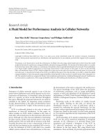
Figure 4: Run length histogram of a BOC(5, 3) signal.
(4m − n − 1)/(4m + n − 2) of those intervals are of length T
s
,
and n
− 1 intervals of length (i/n)T
s
, i = 1, , n − 1, appear
with probability 2/(4m + n
− 2).
Resuming, for large p, the relation N(T
s
):N(2T
s
)is
taken from the previous section, that is, 4m
− 2:1follow-
ing the results for BOC(m,1). Next, n

− 1 half periods are
divided into intervals separating phase jumps with duration
(1/n)T
s
, ,((n − 1)/n)T
s
all appearing twice in mean.
As an example, we consider again a BOC(5, 3) signal. The
run length statistics (Figure 4) obtained for this signal show
four different intervals of length T
s
/3, 2T
s
/3, T
s
,and2T
s
with
distributions 2/21, 2/21, 16/21, and 1/21, respectively.
As in the previous section also the latter results can be
extended in a rather straightforward way. In case we are deal-
ing with BOC(m, n)with1< gcd(2m, n) <n,wemaycon-
sider BOC(m/c, n/c), with c
= gcd(2m, n). Since this type
of signals only differs from BOC(m, n) by means of a divi-
sion/multiplication of T
c
and T
s
by c, the same run length

statistics as for BOC(m, n)with1< gcd(2m, n) <napply for
BOC(m/c, n/c). Furtherm ore, we have gcd(2m/c, n/c)
= 1,
so that we can use the previously obtained results. Following
B. Muth et al. 5
these results, we have a portion of c/(4m+n − 2c) of all inter-
vals between phase jumps of length 2T
s
,(4m − n − c)/(4m +
n
− 2c) of those intervals of length T
s
and n/c − 1 intervals
of length i(c/n)T
s
, i = 1, , n/c − 1, appear with probability
2c/(4m + n
− 2c).
Reviewing the five different cases that cover all differ-
ent BOC(m, n), m
≥ n, we observe that every single case
can be regarded as a special case of the latter case in which
1 < gcd(2m, n) <n. Therefore, the run length statistics for
arbitrary BOC(m, n)readasinTable 2.
5. CONVERGENCE AND EXPERIMENTAL
RESULTSFORRUNLENGTHSTATISTICS
In this section, we discuss the results as presented in Table 2
from a practical point of view. First we will derive an ap-
proximation result, that yields an indication of the number
of chips to be taken into account before the steady distribu-

tion of Tab le 2 is achieved up to a given accuracy. Next, ex-
perimental results for different BOC(m, n)willillustrateac-
curacy and correctness of the statistics in prac tice.
The derived statistics hold in case many chips (in time)
are considered at different positions in the signal. However,
the exact number of chips necessary to approximate the
steady distribution does not follow from the derivations in
the previous section. To give insight in this convergence be-
haviour we consider BOC(kn/2, n)-type of signals and derive
an expression for the number of code chips to be considered
before the distribution from Tab le 2 is obtained up to a g iven
accuracy.
For m
= kn/2 we use (6) to get the fraction of 2T
s
run
lengths after p chips, given by
N

2T
s

N

T
s

+ N

2T

s

=
(p − 1)/2
2pm/n − p/2+1/2
=
np − n
4pm − np + n
.
(9)
According to Table 2 ,wehavetocompare(9)with
n/(4m
− n), the fraction’s value in limit. The relative error
in the statistics for N(2T
s
)isnowgivenby
E
m,n
(p) =




n/(4m − n) −

(pn − n)/(4pm − pn + n)

n/(4m − n)





=




1 −
(4m − n)(p − 1)
4pm − pn + n




=




1 −
4pm − pn + n − 4m
4pm − pn + n




=
4m
p(4m − n)+n
.

(10)
The number of chips p to be considered for obtaining an ac-
curacy δ in the relative error is calculated from E
m,n
(p) ≤ δ.
Rewritting this inequality using (10) yields
p>
4m
− δn
4δm − δn
. (11)
We observe that for small δ the minimum number of chips p
needed for accuracy δ tends to
p
≈
4m
δ(4m − n)
. (12)
Table 2: BOC(m, n) run length statistics with c = gcd(2m, n).
Run length Fraction in distribution
i
cT
s
n
, i
= 1, , n/c − 1
2c
4m + n − 2c
T
s

4m − n − c
4m + n − 2c
2T
s
c
4m + n − 2c
10
6
10
5
10
4
10
3
10
2
10
1
Number of chips p needed to reach accuracy δ
10
−6
10
−5
10
−4
10
−3
10
−2
10

−1
Accuracy δ
BOC(1, 1)
BOC(6, 1)
BOC(10, 5)
Figure 5: Number of chips p needed to reach accuracy δ for differ-
ent BOC signals.
Figure 5 depicts the logarithmic dependence of the number
of chips p to the required accuracy δ for different BOC sig-
nals with parameters (1, 1), (6, 1), and (10, 5).
Similar computations also hold for expressing the relative
error in the steady results for N(T
s
). It can be derived (left to
the reader) that for N(T
s
) we have a relative error

E
m,n
(p) =
2mn/(2m − n)
p(4m − n)+n
. (13)
We will not elaborate further on this relative error, since the
error in N(2T
s
) always is the largest and therefore seems to
be the best quality measure for the statistics.
We remark that the results obtained here only hold in

case the expected values for the dist ribution after p chips are
accurate. This can be achieved by taking a large number of p-
chip intervals into account and averaging the distributions.
For several types of BOC(m, n) signals the distr ibutions
of r un lengths have been calculated during a 7- microsecond
simulation. Figure 6 shows the calculated run length dis-
tribution for a simulated BOC(10, 5) signal. As can be
seen in the figure, already a simulation of 36-code chips
yields a result close to the derived steady distribution. Since
6 EURASIP Journal on Advances in Signal Processing
this simulation was only done for a small number of 7-
microsecond t ime inter val, the values of the steady distri-
bution are not accurate enough, resulting in a relative error
E
10,5
(p) that is larger than the theoretical error.
Figure 7 shows the distribution of runs length for a
BOC(7, 3) signal. Since this situation corresponds to the case
where n does not divide 2m more run lengths appear, namely,
T
s
/3, 2T
s
/3, T
s
,and2T
s
. In this experiment, more chips then
in Figure 6 have been considered yielding a better approxi-
mation.

6. CONCLUSIONS AND FUTURE RESEARCH
In this paper, we introduced an identification of a BOC(m, n)
signal through a unique histogram. Indeed, measuring the
duration of time intervals between phase jumps and count-
ing them leads to a distribution depending only on the
BOC parameters m and n. Although similar histograms may
show up for different BOC(m, n), the values of T
s
will dif-
fer in these cases resulting in unique fingerprints. If n di-
vides 2m only subcarrier half periods (T
s
)andfullperi-
ods (2T
s
) are observed in the BOC(m, n) signal with re-
spective probabilities of occurrence (4m
− 2n)/(4m − n)and
n/(4m
− n). Otherwise, if n and 2m are relatively prime,
n + 1 possible run length exist, namely, subcarrier half-
periods (T
s
), full periods (2T
s
) with respective probabilities
(4m
− n − 1)/(4m + n − 2) and 1/(4m + n − 2) and also in-
tervals equal to (iT
s

/n)1, , n − 1 each appearing with a
probability equal to 2/(4m + n
− 2).
The analysis described in this paper can only be p er-
formed in case most phase jumps in the signal can be iden-
tified. In case a reasonably large number of chips are consid-
ered, not having identified some phase jumps is not a huge
problem. This is due to the fact that these mismatches will
disappear when matching steady distributions for classify-
ing the signals. In practice, this means that the method also
can be applied to noisy signals with reasonable SNR values.
Moreover, also the type of BOC(m, n) plays a role in accurate
classification in noisy environments. Small run lengths (high
values of n) and small jumps in the combined BOC signal
may disappear in the noise more easily than other type of
phase jumps. A better description of this topic is subject to
further research.
Further research is also needed to find out whether, with
the same statistical approach, identification of other BOC-
based signals is possible. One can think of the recently in-
troduced MBOC class of signals and BOC signals based
on different spreading waveforms, see [7]. We expect that
our method can be adapted more or less straightforwardly
for time-multiplexed BOC (TMBOC) signals, since this is
a time-domain arrangement of different BOC signals, as
treated in this paper. Since the idea behind our approach is
not affected by the position of the phase jumps, we expect the
method also to be applicable to cosine-phased BOC. How-
ever, more research is needed for finding the exact shape of
the run length histogr ams for variations on BOC signals and

for answering the question of uniqueness of such new statis-
tics.
100
90
80
70
60
50
40
30
20
10
0
Probability of occurrence %
T
s
2T
s
17.5
14.3
82.5
85.7
Run length values
Figure 6: Histogram of the run lengths of a BOC(10, 5) signal of
duration 7 μs (corresponding to 36 code chips). The lighter bars
account for the computed experimental probabilities, whereas the
darker bars make up for the theoretical probabilities.
100
90
80

70
60
50
40
30
20
10
0
Probability of occurrence %
1
3
T
s
2
3
T
s
T
s
2T
s
3.9
3.4
7.3
6.9
7.3
6.9
81.5
82.8
Run length values

Figure 7: Histogram of the run lengths of a BOC(7,3) signal of du-
ration 1 ms (corresponding to 3069 code chips). The lighter bars
account for the computed experimental probabilities, whereas the
darker bars make up for the theoretical probabilities.
REFERENCES
[1] J. W. Betz, “The offset carrier modulation for GPS moderniza-
tion,” in Proceedings of the National Technical Meeting of the In-
stitute of Navigation (ION NTM ’99), pp. 639–648, San Diego,
Calif, USA, January 1999.
[2] G. W. Hein, J A. Avila-Rodriguez, L. Ries, et al., “A candidate
for the Galileo L1 OS optimized signal,” in Proceedings of the
18th International Technical Meeting of the Satellite Division of
the Institute of Navigation (ION GNSS ’05), pp. 833–845, Long
Beach, Calif, USA, September 2005.
[3] J. W. Betz, “Binary offset carrier modulations for radionaviga-
tion,” Journal of The Institute of Navigation,vol.48,no.4,pp.
227–246, 2001.
B. Muth et al. 7
[4]J.K.Holmes,S.Raghavan,P.Dafesh,andS.Lazar,“Effective
signal to noise ratio performance comparison of some GPS
modernization signals,” in Proceedings of the 12th International
Technical Meeting of the Satellite Division of the Institute of Nav-
igation (ION GPS ’99), pp. 1755–1762, Nashville, Tenn, USA,
September 1999.
[5] J A. Avila-Rodriguez, G. W. Hein, S. Wallner, T. Schueler, E .
Schueler, and M. Irsigler, “Revised combined Galileo/GPS fre-
quency and signal performance analysis,” in Proceedings of the
18th International Technical Meeting of the Satellite Division of
the Institute of Navigation (ION GNSS ’05), pp. 846–860, Long
Beach, Calif, USA, September 2005.

[6] Galileo Joint Undertaking, “Galileo Open Service Signal in
Space Interface Control Document (OS SIS ICD) Draft 0,” May
2006.
[7] G. W. Hein, J A. Avila-Rodriguez, S. Wallner, et al., “MBOC:
the new optimized spreading modulation recommended for
Galileo L1 OS and GPS L1C,” in Proceedings of the IEEE/ION
Position, Location, and Navigation Symposium (PLANS ’06),pp.
883–892, San D iego, Calif, USA, April 2006.
B. Muth graduated in June 2005 from the
Electronics Department of the ENSEEIHT
engineering school in Toulouse, France. He
obtained both the engineering degree and
the M.S. degree with specialisation in sig-
nal processing. His M.S. thesis research, car-
ried out at the French-German Institute ISL
of Saint-Louis, France, focused on environ-
mental noise canceling for acoustic localiza-
tion of snipers. Since December 2005, he
is working as a Ph.D. student in a joint project of The Nether-
lands Defense Academy and the Mathematical Geodesy and Posi-
tioning g roup at the Aerospace Engineering Faculty, Delft Univer-
sity of Technology, The Netherlands. His research focuses on time-
frequency digital signal processing solutions for global navigation
satellite systems software receivers.
P. Oonincx received his M.S. degree (with
honors) in mathematics from Eindhoven
University in 1995 with a thesis on gen-
eralizations of multiresolution analysis. In
2000, he received the Ph.D. degree in math-
ematics from University of Amsterdam. His

thesis on the mathematics of joint time-
frequency/scale analysis has also appeared
as a textbook. Currently, he works as an As-
sociate Professor in mathematics and signal
processing at The Netherlands Defense Academy, Den Helder, The
Netherlands. His research interests are GNSSs signal processing,
wavelet analysis, time-frequency signal representations, multires-
olution imaging, and signal processing for geophysics.
C. Tiberius obtained his Ph.D. degree
in 1998 at Delft University of Technol-
ogy on recursive data processing for kine-
matic GPS surveying. His research inter-
est lies in radio-navigation, primarily with
global navigation satellite systems. He is
currently an Assistant Professor in the
Delft Institute of Earth Observation and
Space Systems (DEOS), and responsible for
courses on data processing and navigation.
He is involved in international projects on satellite navigation,
in particular on the European EGNOS augmentation system and
Galileo.