Báo cáo hóa học: "GEOMETRIC AND HOMOTOPY THEORETIC METHODS IN NIELSEN COINCIDENCE THEORY" pdf
Bạn đang xem bản rút gọn của tài liệu. Xem và tải ngay bản đầy đủ của tài liệu tại đây (824.13 KB, 15 trang )
GEOMETRIC AND HOMOTOPY THEORETIC METHODS IN
NIELSEN COINCIDENCE THEORY
ULRICH KOSCHORKE
Received 30 November 2004; Accepted 21 July 2005
In classical fixed point and coincidence theory, the notion of Nielsen numbers has proved
to be extremely fruitful. Here we extend it to pairs ( f
1
, f
2
)ofmapsbetweenmanifolds
of arbitrary dimensions. This leads to estimates of the minimum numbers MCC( f
1
, f
2
)
(and MC( f
1
, f
2
), resp.) of path components (and of points, resp.) in the coincidence sets
of those pairs of maps which are ( f
1
, f
2
). Furthermore we deduce fi niteness conditions
for MC( f
1
, f
2
). As an application, we compute both minimum numbers explicitly in four
concrete geometric sample situations. The Nielsen decomposition of a coincidence set is
induced by the decomposition of a certain path space E( f
1
, f
2
) into path components.
Its higher-dimensional topology captures further crucial geometric coincidence data. An
analoguous approach can be used to define also Nielsen numbers of certain link maps.
Copyright © 2006 Ulr i ch Koschorke. This is an open access article distributed under the
Creative Commons Attribution License, which permits unrestricted use, distribution,
and reproduction in any medium, provided the original work is properly cited.
1. Introduction and discussion of results
Throughout this paper f
1
, f
2
: M → N denote two (continuous) maps between the smooth
connected manifolds M and N without boundary, of strictly positive dimensions m and
n, respectively, M being compact.
We would like to measure how small (or simple in some sense) the coincidence locus
C
f
1
, f
2
:=
x ∈ M | f
1
(x) = f
2
(x)
(1.1)
canbemadebydeforming f
1
and f
2
via homotopies. Classically one considers the
minimum number of coincidence points
MC
f
1
, f
2
:= min
#C
f
1
, f
2
|
f
1
∼ f
1
, f
2
∼ f
2
(1.2)
(cf. [1], (1.1)). It coincides with the minimum number min
{#C( f
1
, f
2
) | f
1
∼ f
1
} where
only f
1
is modified by a homotopy (cf. [2]). In particular, in topological fixed point theory
Hindawi Publishing Corporation
Fixed Point Theory and Applications
Volume 2006, Article ID 84093, Pages 1–15
DOI 10.1155/FPTA/2006/84093
2 Methods in Nielsen coincidence theory
(where M
= N and f
2
is the identity map) this minimum number is the principal object
of study (cf. [3, page 9]).
In higher codimensions, however, t he coincidence locus is generically a manifold of
dimension m
− n>0, and MC( f
1
, f
2
) is often infinite (see, e.g., Examples 1.4 and 1.6
below). Thus it seems more meaningful to study the minimum number of coincidence
components
MCC
f
1
, f
2
:= min
#π
0
C
f
1
, f
2
|
f
1
∼ f
1
, f
2
∼ f
2
, (1.3)
where #π
0
(C( f
1
, f
2
)) denotes the (generically finite) number of path components of the
indicated coincidence subspace of M.
Question 1.1. How big are MCC( f
1
, f
2
)andMC(f
1
, f
2
)? In particular, when do these in-
variants vanish, that is, when can the maps f
1
and f
2
be deformed away from one another?
In this paper, we discuss lower bounds for MCC( f
1
, f
2
) and geometric obstructions to
MC( f
1
, f
2
) being trivial or finite.
A careful investigation of the differential topology of generic coincidence submanifolds
yields the normal bordism classes (cf. (4.6)and(4.7))
ω
f
1
, f
2
∈
Ω
m−n
(M;ϕ),
ω
f
1
, f
2
∈
Ω
m−n
E
f
1
, f
2
; ϕ
(1.4)
as well as a sharper (“nonstabilized”) version
ω
#
f
1
, f
2
∈
Ω
#
f
1
, f
2
(1.5)
of
ω( f
1
, f
2
)(cf.Remark 4.2). Here the path space
E
f
1
, f
2
:=
(x, θ) ∈ M × N
I
| θ(0) = f
1
(x), θ(1) = f
2
(x)
(1.6)
(cf. Section 2), also known as (a kind of) homotopy equalizer of f
1
and f
2
,playsacrucial
role. In general it has a very rich topology involving both M and the loop space of N.
Already the set π
0
(E( f
1
, f
2
)) of path components can be huge—it corresponds bijectively
to the Reidemeister set
R
f
1
, f
2
=
π
1
(N)/Reidemeister equivalence (1.7)
(cf. [1, 3.1] and our Proposition 2.1 below) which is of central importance in classi-
cal Nielsen theory. Thus it is only natural to define a “Nielsen number” N( f
1
, f
2
)(and
a sharper version N
#
( f
1
, f
2
), resp.) to be the number of those (“essential”) path com-
ponents which contribute nontr ivially to the bordism class
ω( f
1
, f
2
)(andtoω
#
( f
1
, f
2
),
resp .), compare Definition 4.1 and Remark 4.2.
Ulrich Koschorke 3
Theorem 1.2. (i) The integers N( f
1
, f
2
) and N
#
( f
1
, f
2
) depend only on the homotopy
classes of f
1
and f
2
; (ii) N( f
1
, f
2
) = N( f
2
, f
1
) and N
#
( f
1
, f
2
) = N
#
( f
2
, f
1
); (iii) 0 ≤ N( f
1
,
f
2
) ≤ N
#
( f
1
, f
2
) ≤ MCC( f
1
, f
2
) ≤ MC( f
1
, f
2
); if n = 2,thenalsoMCC( f
1
, f
2
) ≤ #R( f
1
, f
2
);
(iv) if m
= n, then N( f
1
, f
2
) = N
#
( f
1
, f
2
) coincides with the classical Nielsen number (cf. [1,
Definit ion 3.6]).
Remark 1.3. In various situations, some of the estimates spelled out in part (iii) of this
theorem are known to be sharp (compare also [12]). For example, in the self-coincidence
setting (where f
1
= f
2
) we have always MCC( f
1
, f
2
) ≤ 1 (since here C( f
1
, f
2
) = M). In
the “root setting” (where f
2
maps to a constant value ∗∈N) all Nielsen classes are si-
multaneously essential or inessential (since our ω-invariants are always compatible with
homotopies of ( f
1
, f
2
) and hence, in this particular case, with the action of π
1
(N,∗), cf.
the discussion in [12] following (1.10)). Therefore in both settings MCC( f
1
, f
2
) is equal
to the Nielsen number N( f
1
, f
2
)provided ω( f
1
, f
2
) = 0(andn = 2if f
2
≡∗).
Further geometric and homotopy theoretic considerations allow us to determine the
Nielsen and minimum numbers explicitly in several concrete sample situations (for
proofs see Section 6 below).
Example 1.4. Given integers q>1andr,letN
=
C
P(q)beq-dimensional complex pro-
jective space, let M
= S(⊗
r
C
λ
C
) be the total space of the unit circle bundle of the rth tensor
power of the canonical complex line bundle, and let f : M
→ N denote the fiber projec-
tion. Then
N( f , f )
= N
#
( f , f ) = MCC( f , f ) =
⎧
⎨
⎩
0ifq ≡−1(r), q ≡ 1(2),
1else;
MC( f , f )
=
⎧
⎪
⎪
⎪
⎨
⎪
⎪
⎪
⎩
0ifq ≡−1(r), q ≡ 1(2),
1ifq
≡−1(r), q ≡ 0(2),
∞ if q ≡−1(r).
(1.8)
As was shown above (cf. Remark 1.3), in any self-coincidence situation (where f
1
= f
2
)
MCC( f
1
, f
2
) must be 0 or 1 and it remains only to decide which value occurs. In the
previous example this can be settled by the normal bordism class ω( f , f )
∈ Ω
1
(M;ϕ),
aweakformof
ω( f , f ) which, however, captures a delicate (“second order”) Z
2
-aspect
as well as the dual of the classical first order obstruction. Already in this simple case
standard methods of singular (co)homology theory yield only a necessary condition for
MCC( f
1
, f
2
) to vanish (cf. [7, 2.2]). In higher codimensions m − n the advantage of the
normal bordism approach can be truely dramatic.
Example 1.5. Given natural numbers k<r,letM
= V
r,k
(and N = G
r,k
,resp.)bethe
Stiefel manifold of orthonormal k-frames (and the Grassmannian of k-planes, resp.) in
R
r
.Let f : M → N map a frame to the plane it spans.
Assume r
≥ 2k ≥ 2. Then
N( f , f )
= N
#
( f , f ) = MCC( f , f ) = MC( f , f ) =
⎧
⎨
⎩
0ifω( f , f ) = 0,
1else.
(1.9)
4 Methods in Nielsen coincidence theory
Here the normal bordism obstruction ω( f , f )
∈ Ω
m−n
(M;ϕ)(cf.(4.7)) contains precisely
as much information as its “highest order component”
2χ
G
r,k
·
SO(k)
∈
Ω
fr
m
−n
∼
=
π
S
m
−n
, (1.10)
where [SO(k)] denotes the framed bordism class of the Lie group SO(k), equipped with
a left invariant parallelization; the Euler number χ(G
r,k
) is easily calculated: it vanishes
if k
≡ r ≡ 0(2) and equals
[r/2]
[k/2]
otherwise. Without loosing its geometric flavor, our
original question translates here—via the Pontryagin-Thom isomorphism—into deep
problems of homotopy theory (compare the discussion in the introduction of [11]). For-
tunately powerful methods are available in homotopy theory which imply, for example,
that MCC(f , f )
= MC( f , f ) = 0ifk is even or k = 7or9orχ(G
r,k
) ≡ 0(12); however,
if k
= 1andr ≡ 1(2), or if k = 3andr ≡ 1(12) is odd, or if k = 5andr ≡ 5(6), then
MCC( f , f )
= MC( f , f ) = 1.
These results seem to be entirely out of the reach of the methods of singular
(co)homology theory since we would have to deal here with obstr uctions of order m
−
n +1= k(k − 1)/2+1.
Example 1.6. Let N be the torus (S
1
)
n
and let ι
1
, ,ι
n
denote the canonical generators of
H
1
((S
1
)
n
;Z). If the homomorphism
f
1∗
− f
2∗
: H
1
(M;Z) −→ H
1
S
1
n
;Z
(1.11)
has an infinite cokernel (or, equivalently, the rank of its image is strictly smaller than n),
then
N
f
1
, f
2
=
N
#
f
1
, f
2
=
MCC
f
1
, f
2
=
MC
f
1
, f
2
=
0. (1.12)
On the other hand, if the cup product
n
j=1
f
∗
1
− f
∗
2
ι
j
∈
H
n
(M;Z) (1.13)
is nontrivial, then MC( f
1
, f
2
) =∞whenever m>n; if in addition n = 2, then MCC( f
1
, f
2
)
equals the (finite) cardinality of the cokernel of f
1∗
− f
2∗
(cf.(1.11)).
In the special case when N is the unit circle S
1
we ha v e: MCC( f
1
, f
2
) = MC( f
1
, f
2
) =
0iff
1
is homotopic to f
2
; other wise MCC( f
1
, f
2
) = #coker(f
1∗
− f
2∗
), but (if m>1)
MC( f
1
, f
2
) =∞.
Ulrich Koschorke 5
An important special case of our invariants are the degrees
deg
#
( f ):= ω
#
( f ,∗),
deg( f ):=
ω( f ,∗), deg( f ):= ω( f ,∗) (1.14)
of a given map f : M
→ N (here ∗ denotes a constant map).
Example 1.7 (homotopy groups). Let M be the sphere S
m
; in view of the previous example
we may also assume that n
≥ 2.
Then, given [ f
i
] ∈ π
m
(N,∗
i
), i = 1,2, ∗
1
=∗
2
, we can identify Ω
#
( f
1
, f
2
),Ω
m−n
(E( f
1
,
f
2
); ϕ)andΩ
m−n
(M;ϕ) with the corresponding groups in the top line of the diagram
π
m
S
n
∧ Ω(N)
+
stabilize
Ω
fr
m
−n
(ΩN) Ω
fr
m
−n
π
m
(N)
deg
#
deg
deg
(1.15)
(This is possible since the loop space ΩN occurs as a typical fiber of the natural projection
p : E( f
1
, f
2
) → S
m
,cf.[12,Section7],and[13].)
Furthermore, after deforming the maps f
1
and f
2
until they are constant on opposite
half spheres in S
n
,weseethat
ω
f
1
, f
2
=
ω
f
1
,∗
2
+ ω
∗
1
, f
2
, (1.16)
and similarly for ω
#
and ω.
Thus it sufficestostudythedegreemapsindiagram(1.15). They turn out to be group
homomorphisms which commute with the indicated natural forgetful homomorphisms.
It can be shown (cf. [13]) that deg
#
( f ) is (a strong version of) the Hopf-Ganea invari-
ant of [ f ]
∈ π
m
(N) (w.r. to the attaching map of a top cell in N,compare[5, 6.7]), while
deg( f ) is closely related to (weaker) stabilized Hopf-James invariants ([12, 1.14]).
Special case: M
= S
m
, N = S
n
, n ≥ 2. Here deg
#
is injective and we see that
N( f ,
∗) ≤ N
#
( f ,∗) = MCC( f ,∗) =
⎧
⎨
⎩
0iff is null homotopic,
1 otherwise,
(1.17)
for all maps f : S
m
→ S
n
. There are many dimension combinations (m,n), where the
equality N( f ,
∗) = N
#
( f ,∗)isalsovalidforall f or, equivalently, where
deg is injec-
tive (compare, e.g., our Remark 4.2 below or [12, 1.16]). However, if n
= 1,3,7 is odd and
m
= 2n − 1, or if, for example, (m, n) = (8,4),(9,4),(9,3),(10,4),(16,8),(17,8),(10 + n,n)
for 3
≤ n ≤ 11, or (24,6), then there exists a map f : S
m
→ S
n
such that 0 = N( f ,∗) <
N
#
( f ,∗) = 1(compare[12, 1.17]).
Very special case: M
= S
3
,N = S
2
.Here
deg : π
3
S
2
∼
=
Z −→
Ω
fr
1
ΩS
2
∼
=
Z
2
⊕ Z (1.18)
6 Methods in Nielsen coincidence theory
captures the Freudenthal suspension and the classical Hopf invariant of a homotopy class
[ f ]; therefore
deg is injective (and so is deg
#
a fortiori).
On the other hand the invariant deg( f )
∈ Ω
fr
1
∼
=
Z
2
(which does not involve the path
space E( f ,
∗)) retains only the suspension of f . The corresponding homological invariant
μ(deg( f ))
∈ H
1
(S
3
;Z) vanishes altogether.
Finally let us point out that our approach can also be applied fruitfully to study linking
phenomena. Consider, for example, a link map
f
= f
1
f
2
: M
1
M
2
−→ N × R (1.19)
(i.e., the closed manifolds M
1
and M
2
have disjoint images). Just as in the case of two
disjoint closed curves in
R
3
thedegreeoflinkingcanbemeasuredtosomeextendbythe
geometry of the overcrossing locus: it consists of that part of the coincidence locus of the
projections to N,where f
1
is bigger than f
2
(w.r. to the R-coordinate). Here the nor mal
bordism/path space approach yields strong unlinking obstructions which, in addition,
turn out to distinguish a great number of different link homotopy classes. Moreover it
leads to a natural notion of Nielsen numbers for link maps (cf. [10]).
2. The path space E(f
1
,f
2
)
A crucial feature of our approach to Nielsen theory is the central role played by the
space E( f
1
, f
2
). It yields the Nielsen decomposition of coincidence sets in a very natu-
ral geometric fashion. In the defining (1.6) N
I
denotes the space of all continuous paths
θ : I :
= [0,1] → N with the compact—open topology. The starting point/endpoint fibra-
tion N
I
→ N × N pulls back, via the map
f
1
, f
2
: M −→ N × N, (2.1)
to yield the Hurewicz fibration
p : E
f
1
, f
2
−→
M (2.2)
defined by p(x,θ)
= x. Given a coincidence point x
0
∈ M,thefiberp
−1
({x
0
})isjustthe
loop space Ω(N, y
0
) of paths in N starting and ending at y
0
= f
1
(x
0
) = f
2
(x
0
); let θ
0
de-
note the constant path at y
0
.
Proposition 2.1. The sequence of group homomorphisms
···−→π
k+1
M,x
0
f
1∗
− f
2∗
−−−−−→ π
k+1
N, y
0
incl
∗
−−−→ π
k
E
f
1
, f
2
,
x
0
,θ
0
p
∗
−−→ π
k
M,x
0
−→ · · · −→
π
1
M,x
0
(2.3)
is exact. Moreover, the fiber inclusion incl : Ω(N, y
0
) → E( f
1
, f
2
) induces a bijection of the
sets
R
f
1
, f
2
=
π
1
N, y
0
/Reidemeister equivalence −→ π
0
E
f
1
, f
2
, (2.4)
where two classes [θ],[θ
] ∈ π
1
(N, y
0
) = π
0
(Ω(N, y
0
)) are called Reidemeister equivalent if
[θ
] = f
1∗
(τ)
−1
· [θ] · f
2∗
(τ) for some τ ∈ π
1
(M,x
0
).
Ulrich Koschorke 7
The proof is fairly evident. In fact, we are dealing here essentially with the long exact
homotopy sequence of the fibration p.
3. Normal bordism
In this section we recall some standard facts about a geometric language which seems well
suited to describe relevant coincidence phenomena in arbitrary codimensions.
Let X be a topological space and let ϕ be a v irtual real vector bundle over X, that is, an
ordered pair (ϕ
+
,ϕ
−
)ofvectorbundleswrittenϕ = ϕ
+
− ϕ
−
.
Asingularϕ-manifold in X of dimension q is a triple (C,g,
g), where
(i) C is a closed smooth q-dimensional manifold;
(ii) g : C
→ X is a continuous map;
(iii)
g : TC ⊕ g
∗
(ϕ
+
) → g
∗
(ϕ
−
)isastable ve ctor bundle isomorphism (i.e., we can
first add trivial vector bundles of suitable dimensions on both sides).
Two such tri pl es (C
i
,g
i
,g
i
), i = 0,1, are bordant if there exists a compact singular (q +
1)-dimensional ϕ-manifold (B,b,
b)inX with boundary ∂B = C
0
C
1
such that b and b,
when restricted to ∂B, coincide with the corresponding data g
i
and g
i
at C
i
, i = 0,1 (via
vector fields pointing into B along C
0
and out of B along C
1
). The resulting set of bordism
classes, with the sum operation given by disjoint unions, is the qth normal bordism group
Ω
q
(X;ϕ) of X with coefficients in ϕ.
Example 3.1. Let G denote the trivial group or the (special) orthogonal group ( S) O(q
),
q
>q+ 1. For any topological space Y let ϕ
+
be the classifying bundle over BG,pulled
back to X
= Y × BG, w hile ϕ
−
is trivial. Then Ω
q
(X;ϕ) is the standard (stably) framed,
oriented or unoriented qth bordism group of Y (cf., e.g., [4, I.4 and 8]).
For every virtual vector bundle ϕ over a topological space X there are well known
Hurewicz homomorphisms
μ : Ω
q
(X;ϕ) −→ H
q
X;
Z
ϕ
, q ∈ Z, (3.1)
into singular homology with local integer coefficients
Z
ϕ
(which are twisted like the ori-
entation line bundle ξ
ϕ
= ξ
ϕ
+
⊗ ξ
ϕ
−
of ϕ); they map a normal bordism class [C, g, g]tothe
image of the fundamental class [C]
∈ H
q
(C;
Z
TC
) by the induced homomorphism g
∗
.
In most cases μ leadstoabiglossofinformation.Howeverforq
≤ 4 this loss can often
be measured so that explicit calculations of (and in) Ω
q
(X;ϕ) are possible (in particular so
when ϕ is highly nontrivial), see [9, Theorem 9.3]. We obtain for example , the following
lemma.
Lemma 3.2. Assume X is path connected. Then the following hold.
(i)
Ω
0
(X;ϕ)
μ
∼
=
H
0
X;
Z
ϕ
=
⎧
⎨
⎩
Z
if w
1
(ϕ) = 0,
Z
2
else.
(3.2)
8 Methods in Nielsen coincidence theory
(ii) The following sequence is exact:
Ω
2
(X;ϕ)
μ
−→ H
2
X;
Z
ϕ
w
2
(ϕ)
−−−−→ Z
2
δ
1
−−→ Ω
1
(X;ϕ)
μ
−→ H
1
X;
Z
ϕ
−→
0. (3.3)
Here δ
1
(1) is represented by the invariantly parallelized unit circle, together with a c on-
stant map, and
w
1
(ϕ) = w
1
ϕ
+
+ w
1
ϕ
−
,
w
2
(ϕ) = w
2
ϕ
+
+ w
1
ϕ
+
w
1
ϕ
−
+ w
2
ϕ
−
+ w
1
ϕ
−
2
(3.4)
denote Stiefel-Whit ney classes of ϕ.
The setting of (normal) bordism groups provides also a first rate illustration of the
fact that the geometric and differential topology of manifolds on one hand, and homo-
topy theory on the other hand, are often but two sides of the same coin. Indeed, if ϕ
−
allows a complementary vector bundle ϕ
−⊥
(such that ϕ
−
⊕ ϕ
−⊥
is trivial), then the well-
known Pontryagin-Thom construction allows us to interpret Ω
q
(X;ϕ), q ∈ Z, as a (sta-
ble) homotopy group of the Thom space of ϕ
+
⊕ ϕ
−⊥
which consists of the total space
of ϕ
+
⊕ ϕ
−⊥
with one point “added at infinity” (compare, e.g., [4,I,11and12]).Thus
the methods of algebraic topology offer another (and often very powerful) approach to
computing normal bordism groups (cf., e .g., [4, Chapter II]).
Example 3.3. The Thom space of the vector bundle ϕ
=
R
k
over a one-point space is
the sphere S
k
=
R
k
∪ {∞}. Hence the framed bordism group Ω
fr
q
:= Ω
q
({point};ϕ)is
canonically isomorphic to the stable homotopy group π
S
q
:= lim
k→∞
π
q+k
(S
k
)ofspheres.
It is computed and listed, for example, in Toda’s tables (in [14, Chapter XIV]) whenever
q
≤ 19.
For further details and references concerning normal bordism see, for example, [6]or
[9].
4. The invariants
In this section we discuss the invariants
ω( f
1
, f
2
)andN( f
1
, f
2
) based on normal bordism,
as well as their shar per (nonstabilized) versions ω
#
( f
1
, f
2
)andN
#
( f
1
, f
2
). We refer to [12]
for some of the details and proofs (see also [13]).
In the special case when the map ( f
1
, f
2
):M → N × N is smooth and transverse to the
diagonal
Δ
=
(y, y) ∈ N × N | y ∈ N
, (4.1)
the coincidence set
C
= C
f
1
, f
2
=
f
1
, f
2
−1
(Δ) =
x ∈ M | f
1
(x) = f
2
(x)
(4.2)
Ulrich Koschorke 9
C
M
( f
1
,f
2
)
N
N
N
× N
Δ
N
× N
Figure 4.1. A generic coincidence manifold and its normal bundle.
is a smooth submanifold of M. It comes with the maps
E
f
1
, f
2
p
C
g
g
M
(4.3)
defined by g(x)
= x and g(x) = (x,constant path at f
1
(x) = f
2
(x)), x ∈ C.
The normal bundle of C in M is described by the isomorphism
ν(C,M)
∼
=
f
1
, f
2
∗
ν(Δ,N × N)
∼
=
f
∗
1
(TN) | C (4.4)
(see Figure 4.1) which yields
g : TC⊕ f
∗
1
(TN) | C
∼
=
−−→ TM | C. (4.5)
Define
ω
f
1
, f
2
:= [C, g,g] ∈ Ω
m−n
E
f
1
, f
2
; ϕ
, (4.6)
ω
f
1
, f
2
:= [C,g,g] = p
∗
ω
f
1
, f
2
∈
Ω
m−n
(M;ϕ), (4.7)
where
ϕ :
= f
∗
1
(TN) − TM, ϕ := p
∗
(ϕ). (4.8)
Invariants with precisely the same properties can be constructed in general. Indeed,
apply the preceding procedure to a smooth map ( f
1
, f
2
)whichistransversetoΔ and
approximates ( f
1
, f
2
).
Also apply the isomorphism Ω
∗
(E( f
1
, f
2
); ϕ
)
∼
=
Ω
∗
(E( f
1
, f
2
); ϕ)inducedbyasmall
homotopy (cf. [12,3.3])to
ω( f
1
, f
2
)inordertoobtain ω( f
1
, f
2
) and similarly ω( f
1
, f
2
).
10 Methods in Nielsen coincidence theory
Now consider the decomposition
ω
f
1
, f
2
=
ω
A
f
1
, f
2
∈
Ω
m−n
E
f
1
, f
2
; ϕ
=
A
Ω
m−n
(A; ϕ | A) (4.9)
according to the various path components A ∈ π
0
(E( f
1
, f
2
)) of E( f
1
, f
2
).
Definit ion 4.1. A pathcomponent of E( f
1
, f
2
)iscalledessential if the corresponding di-
rect summand of
ω( f
1
, f
2
)isnontrivial.TheNielsen c oincidence number N( f
1
, f
2
)isthe
number of essential path components A
∈ π
0
(E( f
1
, f
2
)).
Since we assume M to be compact, N( f
1
, f
2
) is a finite integer. It vanishes if and only
if
ω( f
1
, f
2
)does.
Remark 4.2. In Figure 4.1 we have neglected an important geometric aspect: C is much
more than just an (abstract) singular manifold with an description of its stable normal
bundle. If we keep track (i) of the fact that C is a smooth submanifold in M, and (ii)
of the nonstabilized isomorphism (4.4), we obtain the sharper invariants ω
#
( f
1
, f
2
)and
N
#
( f
1
, f
2
). Note, however, that the bordism set Ω
#
( f
1
, f
2
) in which ω
#
( f
1
, f
2
) lies has pos-
sibly no group structure—the union of submanifolds may no longer be a submanifold.
Also N
#
( f
1
, f
2
) = 0ifω
#
( f
1
, f
2
) = 0, but the converse may possibly not hold in general—
nulbordisms of individual coincidence components may intersect in M
× I.
However, in the stable range m
≤ 2n − 2, ω
#
( f
1
, f
2
) contains precisely as much infor-
mation as
ω( f
1
, f
2
)does,andN
#
( f
1
, f
2
) = N( f
1
, f
2
).
Let us summarize, we have the (successively weaker) invariants ω
#
( f
1
, f
2
), ω( f
1
, f
2
),
ω( f
1
, f
2
)andμ(ω( f
1
, f
2
)) = Poincar
´
e dual of the cohomological primary obstruction to
deforming f
1
and f
2
away from one another (cf. [8, 3.3]); they are related by the natural
forgetful maps
Ω
#
f
1
, f
2
stabilize
−−−−−→ Ω
m−n
E
f
1
, f
2
; ϕ
p
∗
−−→ Ω
m−n
(M;ϕ)
μ
−→ H
m−n
M;
Z
ϕ
(4.10)
(cf. Remark 4.2,(4.3), and (3.1)). Only ω
#
( f
1
, f
2
)and ω( f
1
, f
2
) involve the path space
E( f
1
, f
2
), thus allowing the definition of the Nielsen numbers N
#
( f
1
, f
2
)andN( f
1
, f
2
).
Example 4.3 the classical dimension setting m
= n. Here the coincidence set
C
f
1
, f
2
=
A∈π
0
(E( f
1
, f
2
))
g
−1
(A) (4.11)
consists generically of isolated points (in this very special situation the stabilizing map
and the Hurewicz homomorphism μ in (4.10) lead to no significant loss of information).
In our approach, each Nielsen class is expressed as an inverse image of some path
component A of E( f
1
, f
2
)(compareProposition 2.1). The corresponding index
ω
A
f
1
, f
2
∈
Ω
0
(A; ϕ | A)
∼
=
⎧
⎨
⎩
Z
if ω
1
(ϕ | A) = 0,
Z
2
else,
(4.12)
Ulrich Koschorke 11
(cf. Lemma 3.2)liesin
Z
2
precisely if w
1
(ϕ | A) = 0 or, equivalently, if for some (and
hence all) x
0
∈ g
−1
(A) there exists a class α ∈ π
1
(M,x
0
)suchthat f
1∗
(α) = f
2∗
(α)but
w
1
(M)(α) = f
∗
1
(w
1
(N))(α)(cf.[12, 5.2]; this agrees with the criterion quoted in [1,page
53 lines 5–6]). If π
1
(N) is commutative, then either the indices of all Nielsen classes are
integers, or they all lie in
Z
2
. However, it is easy to construct examples (e.g., involving
maps from the Klein bottle to the punctured torus) where both types of path components
A
∈ π
0
(E( f
1
, f
2
)) occur.
In any case our approach makes it clear from the outset where the indices of Nielsen
classes must take their values.
In the setting of fixed point theory (where f
2
is the identity map on M = N)thetran-
sition from the
ω-totheω-invariant (cf. (4.6)and(4.7)) which forgets the path space
E( f
1
, f
2
) parallels the transition from Nielsen to Lefschetz theory—with all the loss of
information which this entails.
5. Finiteness conditions for the minimum number MC(f
1
,f
2
)
Consider the following possible conditions concerning the invariants defined in (1.2),
(4.6), and (4.7):
(C1) MC( f
1
, f
2
) ≤ 1;
(C2) MC( f
1
, f
2
)isfinite;
(C3)
ω( f
1
, f
2
) lies in the image of the homomorphism
i
E∗
:=
A
i
A∗
:
A
Ω
fr
m
−n
−→
A
Ω
m−n
(A; ϕ |) = Ω
m−n
E
f
1
, f
2
; ϕ
, (5.1)
where direct summation is taken over all A
∈ π
0
(E( f
1
, f
2
)) and i
A∗
is induced by
the inclusion of a point z
A
into the path component A (and by a local orientation
of
ϕ at z
A
);
(C4) ω( f
1
, f
2
) lies in the image of a similarly defined homomorphism
i
∗
: Ω
fr
m
−n
−→ Ω
m−n
(M;ϕ). (5.2)
Proposition 5.1. Each of the first three conditions implies the next one.
Proof. Assume that the coincidence set C( f
1
, f
2
) is finite. If a generic pair ( f
1
, f
2
) approx-
imates ( f
1
, f
2
) closely enough then each component of C( f
1
, f
2
) lies in a ball neighbour-
hood of some x
∈ C( f
1
, f
2
); moreover the corresponding paths which occur in the con-
struction of
ω( f
1
, f
2
) lie entirely in a ball neighbourhood of y = f
1
(x) = f
2
(x) and hence
can be contracted into the constant path at y. Thus (C2) implies (C3). T he proposition
follows.
Our coincidence invariants ω( f
1
, f
2
)andω( f
1
, f
2
) project to the obstructions
ω
f
1
, f
2
∈
coker
i
E∗
,
ω
f
1
, f
2
∈
cokeri
∗
,
(5.3)
which must vanish if MC( f
1
, f
2
)istobefinite.
12 Methods in Nielsen coincidence theory
For m
− n = 0 these cokernels are trivial, MC( f
1
, f
2
) is actually finite and each integer
d
≥ 0 can occur as the value of this minimum number for a suitable pair of maps (e.g.,
for self maps of degrees d and 0 on S
1
).
If m
− n = 1thecokernelsin(5.3) are isomorphic—via the Hurewicz homomorphism
μ (cf. (3.1))—to H
1
(E( f
1
, f
2
);
Z
ϕ
)andH
1
(M;
Z
ϕ
), respectively, (compare Lemma 3.2). In
fact μ vanishes on the image of i
E∗
and of i
∗
, respectively, whenever m − n ≥ 1, but in
general the resulting homomorphisms on the cokernels will not be injective when m
− n>
1(cf.[12, 9.3]).
Remark 5.2. The finiteness criterion in Proposition 5.1 can be sharpened to yield a non-
stabilized version involving ω
#
( f
1
, f
2
).
For self-coincidences there i s a partial converse of Proposition 5.1.
Theorem 5.3. If m<2n
− 2 and f
1
is homotopic to f
2
,thenthefourconditions(C1)–(C4)
are equivalent.
Proof. These conditions are compatible with homotopies of f
1
and f
2
(cf. [12,3.3]and
the discussion following (4.4)). Hence we may assume that f
1
= f
2
=: f .
Recall that the self-coincidence invariant ω( f , f ) is just the singularity obstruction
ω(
R
, f
∗
(TN)) to sectioning the vector bundle f
∗
(TN)overM without zeroes (cf. [11,
Theorem 2.2]).
Now assume that m<2n
− 2andω( f , f ) = i
∗
(ω
0
)forsomeω
0
∈ Ω
fr
m
−n
∼
=
π
S
m
−n
.Then
there exists a map u
∂
: S
m−1
→ S
n−1
whose (stable) Freudenthal suspension corresponds
to ω
0
. Now consider the trivial bundle f
∗
(TN) | B
m
over some compact ball B
m
in M
and interpret u
∂
as a nowhere zero section over ∂B
m
= S
m−1
.
We w ill extend u
∂
to a section u of f
∗
(TN)overall of M which vanishes only in the
centre point of B
m
.OvertheballB
m
we use the obvious “concentric” extension. Note,
however, that generically the zero set of any extension of u
∂
over B
m
is a framed manifold
which represents ω
0
. Thus a generic extension of u
∂
to the complement M −
◦
B
m
must
have a nulbordant manifold of zeroes (representing ω( f , f )
− i
∗
(ω
0
) = 0). According to
[9, Theorem 3.7] these zeroes can be removed altogether.
The resulting section u of f
∗
(TN) allows us to construct a “small” homotopy of f :
for every x
∈ M just deform f (x) somewhat in the direction of the tangent vector u(x) ∈
T
f (x)
(N). We obtain a map which has only one coincidence point with f .
6. The examples of the introduction
In view of the self-coincidence theorem in [11] and of our Theorem 5.3 the first example
is a special case of the following proposition.
Proposition 6.1. Let ξ be an oriented real plane bundle over a closed smooth connected
manifold N and let f : M :
= S(ξ) → N denote the projection of the corresponding unit circle
bundle. Then, the following exist:
(i) the self-coincidence invariant ω( f , f ) (cf. (4.7)) vanishes if and only if the Euler
number χ(N) of N lies in e(ξ)(H
2
(N;Z)) ⊂ Z and χ(N) is even; here e(ξ) denotes
the Euler class of ξ,
Ulrich Koschorke 13
(ii) the finiteness obstr uction μ(ω( f , f ))
[ω( f , f )] (cf. (5.3)andthesubsequentdis-
cussion in Section 5) vanishes if and only if χ(N)
∈ e(ξ)(H
2
(N;Z)).
Proof. We will extend the arguments of [11, Section 4]. Consider the commuting diagram
χ(N)
∈
Z
2
ω( f , f )
∈
incl
∗
Ω
2
(N;−ξ)
μ
Ω
fr
0
(N)
∂
Ω
1
M;− f
∗
(ξ)
μ
H
2
(N;Z)
e(ξ)
w
2
(ξ)
Z
H
1
(M;Z)
Z
2
0
(6.1)
Here the vertical exact sequences are as described in Lemma 3.2. The horizontal lines
are exact Gysin sequences of ξ in normal bordism and in homology (or, equivalently,
oriented bordism), compare [9, 9.20 and 9.4]. As was shown in [11,Section4],wehave
ω( f , f )
= χ(N) · ∂(1). Since the Stiefel-Whitne y class w
2
(ξ) is the mod2 reduction of
e(ξ), the proposition follows.
Next let us examine Example 1.5.Ifr ≥ 2k ≥ 2 then according to the theorem in the in-
troduction of [11] only the “highest order part” 1.11 of the complete obstruction ω( f , f )
(to deforming f away from itself) survives. Thus the finiteness obstruction [ω( f , f )] (cf.
(5.3)) vanishes. If also k
≥ 2thenitfollowsfromTheorem 5.3 that MC( f , f )(andhence
also MCC( f , f )) equals 0 or 1 according to whether ω( f , f ) vanishes or not. It requires
using deep results of homotopy theory and of other branches of algebraic topology to de-
cide which of the two values occur actually, but it can be done at least for k
≤ 10 (cf. [11,
Section 3]). However, the case k
= 1(wherewedealwiththestandardprojectionfrom
S
r−1
to real projective space) is elementary.
Next we turn to Example 1.6 where N
= (S
1
)
n
. Use the Lie group structure to replace
( f
1
, f
2
) by the pair ( f ,∗) which consists of the quotient f = f
1
· f
−1
2
and of the constant
map taking values at the unit element of (S
1
)
n
. This does not change the coincidence sets
and data significantly.
Since each torus (S
1
)
k
is a K(Z
k
,1)-space the homotopy class of f is determined by f
∗
:
H
1
(M;Z) → H
1
((S
1
)
n
;Z). Moreover, if the image of f
∗
has rank k<n,then f factors up
to homotopy through the lower-dimensional torus (S
1
)
k
and hence through (S
1
)
n
−{∗}.
On the other hand, if the image of f
∗
has rank n (or, equivalently, the Reidemeister set
R( f ,
∗)
∼
=
coker f
∗
is finite) then—according to Remark 1.3—all Reidemeister classes are
essential and hence N( f ,
∗) = #R( f ,∗), provided ω( f ,∗) = 0. This holds, in particular,
14 Methods in Nielsen coincidence theory
if the invariant
ω(coll
◦ f ,∗) ∈ Ω
m−n
(M;−TM) (6.2)
which corresponds to the bordism class of the stably coframed manifold C( f ,
∗) =
f
−1
({∗}) ⊂ M,isnontrivial.Herethemap
coll : N
=
S
1
n
−→ N/
N −
◦
B
∼
=
S
n
(6.3)
collapses the complement of an open ball to a point. The induced cohomology homomor-
phisms coll
∗
,and(f ◦ coll)
∗
, respectively, map a generator of H
n
(S
n
;Z) to the cup prod-
uct ι
1
···ι
n
∈ H
n
((S
1
)
n
;Z), and to t he Poincar
´
e dual of μ(ω( f ,∗)), respectively, (compare
(4.10)and[8, 3.3]). Our claims concerning Example 1.6 in the introduction follow now
from Section 5.
Finally note that the facts described in Example 1.7 follow mainly from the discussion
in [12] (see 1.14–1.17 as well as Sections 7 and 8); the calculation of Ω
fr
1
(ΩS
2
)canbe
understood easily with the help of our Lemma 3.2.
Let us put the role of the path space E( f
1
, f
2
) and its influence on the relative strength
of our invariants into perspective (compare diagram (4.10)).
In the self coincidence situation f
1
= f
2
:= f the fibration p : E( f , f ) → M allows a
global section s by constant paths; therefore
ω( f , f ) = s
∗
(ω( f , f )) is precisely as strong
as the (usually much weaker) invariant ω( f , f ) which does not involve any path space
data. As Examples 1.4 and 1.5 illustrate, ω( f , f ) may nevertheless capture decisive and
very delicate information (which is also registered to some extend by the Nielsen number
N( f , f ) in spite of the fact that it can take only the values 0 and 1).
In Example 1.6 our path space approach serves to decompose coincidence sets into
Nielsen classes. However, it does not seem to enrich the higher-dimensional homotopy
theoretical aspects of their data very much (as the torus is aspherical; compare Proposition
2.1). Still, all natural numbers can occur here as Nielsen numbers of suitable maps f
1
and
f
2
.
In contrast, in Example 1.7 the higher-dimensional topology of E( f
1
, f
2
) turns out to
be potentially very rich (e.g., when N
= S
n
, n ≥ 2) and able to capture much more than
just the decomposition into Nielsen classes.
Acknowledgment
This work was supported in part by the Deutsche Forschungsgemeinschaft and AARMS
(Canada).
References
[1] S. A. Bogaty
˘
ı, D. L. Gonc¸alves, and H. Zieschang, Coincidence theory: the minimization problem,
Proceedings of the Steklov Institute of Mathematics 225 (1999), no. 2, 45–77.
[2] R.B.S.Brooks,On removing coincide nces of two maps when only one, rather than both, of them
may be deformed by a homotopy, Pacific Journal of Mathematics 40 (1972), no. 1, 45–52.
Ulrich Koschorke 15
[3] R. F. Brown, Wecken properties for manifolds, Nielsen Theory and Dynamical Systems (Mass,
1992), Contemp. Math., vol. 152, American Mathematical Society, Rhode Island, 1993, pp. 9–
21.
[4] P. E . Conner and E. E. Floyd, Differentiable Periodic Maps, Ergebnisse der Mathematik und ihrer
Grenzgebiete, N. F., vol. 33, Academic Press, New York; Springer, Berlin, 1964.
[5] O. Cornea, G. Lupton, J. Oprea, and D. Tanr
´
e, Lusternik-Schnirelmann Category, Mathematical
Surveys and Monographs, vol. 103, American Mathematical Society, Rhode Island, 2003.
[6] J P. Dax,
´
Etude homotopique des espaces de plongements, Annales Scientifiques de l’
´
Ecole Nor-
male Sup
´
erieure. Quatri
`
eme S
´
erie (4) 5 (1972), 303–377 (French).
[7] A.DoldandD.L.Gonc¸alves, Self-coincidence of fibre maps, Osaka Journal of Mathematics 42
(2005), no. 2, 291–307.
[8] D.L.Gonc¸alves, J. Jezierski, and P. Wong, Obstruction theory and coincidences in positive codi-
mension, Bates College, preprint, 2002.
[9] U. Koschorke, Vector Fields and Other Vector Bundle Morphisms—a Singularity Approach,Lecture
Notes in Mathematics, vol. 847, Springer, Berlin, 1981.
[10]
, Linking and coincidence invariants, Fundamenta Mathematicae 184 (2004), 187–203.
[11]
, Selfcoincidences in higher codimensions,Journalf
¨
ur die Reine und Angewandte Mathe-
matik 576 (2004), 1–10.
[12]
, Nielsen coincidence theory in arbitrary codimensions, to appear in to appear in Jour-
nal f
´
’ur die Reine und Angewandte Mathematik, 2003, http:/www.math.uni-siegen.de/topology/
publications.html.
[13]
, Nonstabilized Nielsen coincidence invariants and Hopf-Ganea homomorphisms, preprint,
2005, />[14] H. Toda, Composition Methods in Homotopy Groups of Spheres, Annals of Mathematics Studies,
no. 49, Princeton University Press, New Jersey, 1962.
Ulrich Koschorke: Universit
¨
at Siegen, Emmy Noether Campus, Walter-Flex Street 3,
D-57068 Siegen, Germany
E-mail address: