Báo cáo hóa học: "A TRANSMISSION PROBLEM FOR BEAMS ON NONLINEAR SUPPORTS" doc
Bạn đang xem bản rút gọn của tài liệu. Xem và tải ngay bản đầy đủ của tài liệu tại đây (567.74 KB, 14 trang )
A TRANSMISSION PROBLEM FOR BEAMS
ON NONLINEAR SUPPORTS
TO FU MA AND HIGIDIO PORTILLO OQUENDO
Received 20 October 2005; Revised 10 April 2006; Accepted 12 April 2006
A transmission problem involving two Euler-Bernoulli equations modeling the vibrations
of a composite beam is studied. Assuming that the beam is clamped at one extremity,
and resting on an elastic bearing at the other extremity, the existence of a unique global
solution and decay rates of the energy are obtained by adding just one damping device at
the end containing the bearing mechanism.
Copyright © 2006 T. F. Ma and H. Portillo Oquendo. This is an open access article dis-
tributed under the Creative Commons Attribution License, which permits unrestricted
use, distribution, and reproduction in any medium, provided the original work is prop-
erly cited.
1. Introduction
In this paper we consider the existence of a global solution and decay rates of the en-
ergy for a transmission problem involving two Euler-Bernoulli equations with nonlinear
boundary conditions. More precisely, we are concerned with the system of equations
ρ
1
u
tt
+ β
1
u
xxxx
= 0in
0,L
0
× R
+
, (1.1)
ρ
2
v
tt
+ β
2
v
xxxx
= 0in
L
0
,L
× R
+
, (1.2)
coupled by the “transmission” conditions
u
L
0
,t
−
v
L
0
,t
=
0, u
x
L
0
,t
−
v
x
L
0
,t
=
0,
β
1
u
xx
L
0
,t
−
β
2
v
xx
L
0
,t
=
0, β
1
u
xxx
L
0
,t
−
β
2
v
xxx
L
0
,t
=
0.
(1.3)
To the system we add the nonlinear boundary conditions
u(0,t)
= 0, u
x
(0,t) = 0, (1.4)
v
xx
(L,t) = 0, β
2
v
xxx
(L,t) = f
v(L,t)
+ g
v
t
(L,t)
, (1.5)
Hindawi Publishing Corporation
Boundary Value Problems
Volume 2006, Article ID 75107, Pages 1–14
DOI 10.1155/BVP/2006/75107
2 A transmission problem for beams on nonlinear supports
0
uv
L
0
L
Bearing
Figure 1.1. A composite beam on an elastic bearing.
and the initial data
u(x,0)
= u
0
(x), u
t
(x,0) = u
1
(x)in
0,L
0
,
v(x,0)
= v
0
(x), v
t
(x,0) = v
1
(x)in
L
0
,L
.
(1.6)
The system (1.1)–(1.6) models the transverse vibrations of a composite beam of length
L, constituted by two types of materials of different mass densities ρ
1
, ρ
2
> 0andflexural
rigidities β
1
,β
2
> 0. Because of the boundary condition (1.4), the beam is clamped at
the left end x
= 0. On the other extremity, the condition (1.5) implies that the bending
moment is zero and that the shear force is equal to f (v(L,t)) + g(v
t
(L,t)). This means
that, at the end x
= L, the beam is resting on a kind of bearing, described by the function
f , and subjected to a frictional dissipation described by the function g (see Figure 1.1).
We notice that stabilization of transmission problems has been considered by some
authors. In the beginning , Lions [8] studied the exact controllability of the transmission
problem for the wave equation. Later, Liu and Williams [10] studied the boundary sta-
bilization of transmission problems for linear systems of wave equations. In the case of
beam equations, which involve fourth-order derivatives, there are more possibilities in
the problem modeling and boundary conditions. For instance, Mu
˜
noz Rivera and Por-
tillo Oquendo [14] studied a transmission problem for viscoelastic beams, by exploiting
the dissipations due to the memory effects of the material. On the other hand, there are
a few results on fourth-order equations with nonlinear boundary conditions involving
third-order derivatives. That class of problems models elastic beams on elastic bearings,
and one of the first results, with nonlinearities, was given by Feireisl [2], who studied
the periodic solutions for a superlinear problem. Some related stationary problems were
considered by Grossinho and Ma [3]andMa[11]. We refer the reader to [1, 4–7, 12–16]
for other interesting related works.
Our objective is to show that under suitable assumptions, the sole dissipation g(v
t
),
acting on the boundary point x
= L,willbesufficient to stabilize the whole system. The
dissipation effect on the boundary x
= L will be transmitted to (1.1)through(1.2). The
proof of the boundary stabilization is based on the arguments from Lagnese [6]and
Lagnese and Leugering [7].
The paper is organized as follows. In Section 2 we define s ome notations and establish
the global existence and uniqueness results (see Theorem 2.2). Weak solutions are also
considered (see Theorem 2.6). In Section 3 we prove the decay of the energy of the system,
T. F. Ma and H. Portillo Oquendo 3
which is defined by
E(t)
= E(t,u,v) =
1
2
L
0
0
ρ
1
u
t
+ β
1
u
xx
dx
+
1
2
L
L
0
ρ
2
v
t
+ β
2
v
xx
dx +
f
v(L,t)
,
(1.7)
where
f (w) =
w
0
f (s)ds (see Theorem 3.1).
2. Global existence
In our study we assume that f is a C
1
function satisfying the sign condition
f (w)w
≥ 0, ∀w ∈ R, (2.1)
and that g is a C
1
for which there exists a constant c
0
> 0suchthat
g(0)
= 0,
g(r)− g(s)
(r − s) ≥ c
0
|r − s|
2
, ∀r,s ∈ R. (2.2)
In particular it follows that g(w)w
≥ c
0
w
2
for all w ∈ R. In order to deal with the trans-
mission conditions (1.3) and the boundary condition (1.4), we define the Sobolev space
X
=
(ϕ,ψ) ∈ H
2
| (ϕ, ψ) satisfies (2.4)
, (2.3)
where
ϕ(0)
= ϕ
x
(0) = ϕ
L
0
−
ψ
L
0
=
ϕ
x
L
0
−
ψ
x
L
0
=
0, (2.4)
H
k
= H
k
0,L
0
×
H
k
L
0
,L
. (2.5)
We also write
L
2
= L
2
(0,L
0
) × L
2
(L
0
,L). Our study is based on the space
V
=
(ϕ,ψ) ∈
H
2
0,L
0
×
H
3
L
0
,L
∩
X | ψ
xx
(L) = 0
, (2.6)
so that the first part of condition (1.5)isalsorecovered.Asasimpleconsequenceofthe
trace theorem and (2.4) one has the following useful boundary estimate.
Lemma 2.1. Given (u,v)
∈ C
1
([0,T],X), there exists a constant C>0 such that
v(L,t)
≤
C
u
xx
2
+
v
xx
2
, ∀t ∈ [0,T],
v
t
(L,t)
≤
C
u
xxt
2
+
v
xxt
2
, ∀t ∈ [0,T],
(2.7)
where
·
2
denotes either L
2
(0,L
0
) or L
2
(L
0
,L) norms.
Now we prove the existence of global regular solutions.
4 A transmission problem for beams on nonlinear supports
Theorem 2.2. Assume that conditions (2.1)-(2.2) hold. Then for any initial data (u
0
,v
0
) ∈
H
4
∩ V and (u
1
,v
1
) ∈ V, satisfying the compatibility condition,
v
0
xxx
(L) − f
v
0
(L)
−
g
v
1
(L)
=
0,
β
1
u
0
xx
L
0
,t
−
β
2
v
0
xx
L
0
,t
=
0,
β
1
u
0
xxx
L
0
,t
−
β
2
v
0
xxx
L
0
,t
=
0,
(2.8)
problem (1.1)–(1.6)hasauniquestrongsolution(u,v) such that
(u,v)
∈ L
∞
R
+
;H
4
,
u
t
,v
t
∈
L
∞
R
+
;X
,
u
tt
,v
tt
∈
L
∞
R
+
;L
2
. (2.9)
The proof of Theorem 2.2 is given in several steps, by using the Galerkin method.
Approximate pr oblem. Let
{(ϕ
n
,ψ
n
)}
n∈N
be a Galerkin basis of V , which for convenience
is chosen to satisfy
u
0
,v
0
,
u
1
,v
1
⊂
V
2
, (2.10)
where
V
m
= span
ϕ
1
,ψ
1
, ,
ϕ
m
,ψ
m
. (2.11)
Then the corresponding approximate variational problem to problem (1.1)–(1.6)reads
as follows: find (u
m
(t),v
m
(t)) ∈ V
m
of the form
u
m
(t),v
m
(t)
=
m
j=1
h
m
j
(t)
ϕ
j
,ψ
j
(2.12)
such that
L
0
0
ρ
1
u
m
tt
ϕ
j
+ β
1
u
m
xx
ϕ
j
xx
dx +
L
L
0
ρ
2
v
m
tt
ψ
j
+ β
2
v
m
xx
ψ
j
xx
dx
+
β
2
f
v
m
(L,t)
+ g
v
m
t
(L,t)
ψ
j
(L) = 0,
(2.13)
u
m
(0),v
m
(0)
=
u
0
,v
0
,
u
m
t
(0),v
m
t
(0)
=
u
1
,v
1
. (2.14)
As a matter of fact, (2.13)isanm-dimensional system of ODEs in h
m
j
(t)andhasalocal
solution (u
m
(t),v
m
(t)) in an interval [0,t
m
]. In the following, we derive uniform esti-
mates, so that local solutions can be extended to the interval [0,T]foranyT>0. Note
that initial conditions in (2.14) are well defined because of (2.10).
Estimate 2.3. Replacing ϕ
i
by u
m
t
and ψ
i
by v
m
t
in (2.13), one concludes that
d
dt
E
t,u
m
,v
m
=−
β
2
g
v
m
t
(L,t)
v
m
t
(L,t). (2.15)
T. F. Ma and H. Portillo Oquendo 5
Then from condition (2.2)weseethatE(t, u
m
,v
m
) is decreasing and therefore there exists
M
1
> 0suchthat
u
m
t
(t)
2
2
+
v
m
t
(t)
2
2
+
u
m
xx
(t)
2
2
+
v
m
xx
(t)
2
2
≤ M
1
(2.16)
for all m
∈ N, t>0, where M
1
depends on E(0,u
0
,v
0
).
Estimate 2.4. Letusobtainanestimateforu
m
tt
(0) and v
m
tt
(0) in L
2
norms. Replacing ϕ
i
by
u
m
tt
(0) and ψ
i
by v
m
tt
(0) in (2.13), one concludes from the compatibility condition (2.8)
that for some constant C>0,
u
m
tt
(0)
2
2
+
v
m
tt
(0)
2
2
≤ C
u
0
xxxx
2
2
+
v
0
xxxx
2
2
. (2.17)
Therefore, there exists M
= M(u
0
,v
0
) > 0suchthat
u
m
tt
(0)
2
2
+
v
m
tt
(0)
2
2
≤ M (2.18)
for all m
∈ N.
Estimate 2.5. Here we use a finite-difference argument as in [12]. Let us fix t, ξ>0such
that ξ<T
− t, and take the difference of (2.13)witht = t + ξ and t = t.Thenreplacingϕ
j
by u
m
t
(t + ξ) − u
m
t
(t)andψ
j
by v
m
t
(t + ξ) − v
m
t
(t), and putting
P
m
(t,ξ) = ρ
1
u
m
t
(t + ξ) − u
m
t
(t)
2
2
+ ρ
2
v
m
t
(t + ξ) − v
m
t
(t)
2
2
+ β
1
u
m
xx
(t + ξ) − u
m
xx
(t)
2
2
+ β
2
v
m
xx
(t + ξ) − v
m
xx
(t)
2
2
,
(2.19)
one infers that
1
2
d
dt
P
m
(t,ξ) ≤ A + B, (2.20)
where
A
=−
g
v
m
(L,t + ξ)
−
g
v
m
(L,t)
v
m
t
(L,t + ξ) − v
m
t
(L,t)
,
B
=−β
2
f
v
m
(L,t + ξ)
−
f
v
m
(L,t)
v
m
t
(L,t + ξ) − v
m
t
(L,t)
.
(2.21)
Taking 0 <ε<c
0
, and using the mean value theorem and Lemma 2.1, there exists C
ε
> 0
such that
B
≤ C
ε
u
m
xx
(t + ξ) − u
m
xx
(t)
2
2
+
v
m
xx
(t + ξ) − v
m
xx
(t)
2
2
+ ε
v
m
t
(L,t + ξ) − v
m
t
(L,t)
2
.
(2.22)
Then from condition (2.2), we conclude that for a constant C>0,
1
2
d
dt
P
m
(t,ξ) = C
P
m
(t,ξ), (2.23)
6 A transmission problem for beams on nonlinear supports
and therefore
P
m
(t,ξ) ≤
P
m
(0,ξ)e
2CT
. So, dividing the inequality by ξ
2
and making ξ → 0,
we see that
ρ
1
u
m
tt
(t)
2
2
+ ρ
2
v
m
tt
(t)
2
2
+ β
1
u
m
xxt
(t)
2
2
+ β
2
v
m
xxt
(t)
2
2
≤
ρ
1
u
m
tt
(0)
2
2
+ ρ
2
v
m
tt
(0)
2
2
+ β
1
u
1
xx
2
2
+ β
2
v
1
xx
2
2
e
CT
.
(2.24)
Hence there exists M
2
> 0suchthat
u
m
tt
(t)
2
2
+
v
m
tt
(t)
2
2
+
u
m
xxt
(t)
2
2
+
v
m
xxt
(t)
2
2
≤ M
2
(2.25)
for all m
∈ N and t ∈ [0,T].
Existence result. From Estimates 2.3 and 2.5, we can apply Aubin-Lions compactness the-
orem to pass to the limit the approximate problem. Then the proof of the existence result
is complete.
Uniqueness. Let (u
1
,v
1
)and(u
2
,v
2
)betwosolutionsofproblem(1.1)–(1.6). Writing
U
= u
1
− u
2
and V = v
1
− v
2
,weseethat(U,V) satisfies
1
2
d
dt
ρ
1
U
t
(t)
2
2
+ ρ
2
V
t
(t)
2
2
+ β
1
U
xx
(t)
2
2
+ β
2
V
xx
(t)
2
2
≤−
β
2
f
v
1
(L,t)
−
f
v
2
(L,t)
V
t
(L,t)
− β
2
g
v
1t
(L,t)
−
g
v
2t
(L,t)
V
t
(L,t).
(2.26)
Then using (2.2)andLemma 2.1,asinEstimate 2.5, we deduce the existence of C>0
such that
d
dt
P(t)
≤ C
U
xx
(t)
2
2
+
V
xx
(t)
2
2
, t ∈ [0,T], (2.27)
where now P(t)
= P(U,V,t). Since we have P(0) = 0, from Gronwall lemma we get U =
V = 0.
Weak solutions. We say that a pair (u,v)isaweaksolutionofproblem(1.1)–(1.6)if
(u,v)
∈ L
∞
R
+
,X
,
u
t
,v
t
∈
L
∞
R
+
,L
2
,
u
tt
,v
tt
∈
L
∞
R
+
,H
−2
(2.28)
satisfy the initial conditions (1.6), the compatibility conditions (2.8), and the variational
identity
d
dt
L
0
0
ρ
1
u
t
ϕdx+
L
L
0
ρ
2
v
t
ψdx
+
L
0
0
β
1
u
xx
ϕ
xx
dx +
L
L
0
β
2
v
xx
ψ
xx
dx +
β
2
f
v(L,t)
+ g
v
t
(L,t)
ψ(L) = 0
(2.29)
T. F. Ma and H. Portillo Oquendo 7
for all (ϕ,ψ)
∈ X. In order to study the existence of weak solutions let us denote by Ꮿ the
set of all acceptable initial data for the existence of strong solutions, that is,
Ꮿ :
=
u
0
,v
0
,
u
1
,v
1
∈
H
4
∩ V
×
V | (2.8)holds
. (2.30)
Then we have the following existence result for weak solutions.
Theorem 2.6. Assume that conditions (2.1)-(2.2) hold. Then for any initial data satisfying
u
0
,v
0
,
u
1
,v
1
∈
Ꮿ
H
2
×L
2
, (2.31)
problem (1.1)–(1.6)hasauniqueweaksolution.
This theorem is proved using density arguments, similar to those used by Cavalcanti
et al. [1]. In fact, from the assumption on the initial data, there exists a sequence ((u
0
ν
,v
0
ν
),
(u
1
ν
,v
1
ν
)) ∈ Ꮿ such that
u
0
ν
,v
0
ν
−→
u
0
,v
0
in H
2
,
u
1
ν
,v
1
ν
−→
u
1
,v
1
in L
2
. (2.32)
Now, for each ν
∈ N, the initial conditions (u
0
ν
,v
0
ν
)and(u
1
ν
,v
1
ν
) give a unique regular solu-
tion (u
ν
,v
ν
)ofproblem(1.1)–(1.6). From the estimates used in the proof of Theorem 2.2
it can be shown that (u
ν
,v
ν
) converges to a weak solution (u,v)of(1.1)–(1.6). The unique-
ness is then proved by means of the regularization techniques as by Lions and Visik (see
e.g. [9]).
3. Decay of the energy
In this section we study decay rates for the first-order energy (1.7) associated to system
(1.1)–(1.6). Here we assume that the bearing device has a superlinear behavior, charac-
terized by the condition
∃ρ ≥ 2suchthatρ
f (w) − f (w)w ≤ 0, ∀w ∈ R, (3.1)
and that t he material of the beam occupying [L
0
,L]ismoredenseandstiff than that in
[0,L
0
], that is,
ρ
1
≤ ρ
2
, β
1
≥ β
2
. (3.2)
Then the rate of decay will depend on the behavior of the nonlinear dissipation g in
a neighborhood of the origin, which is related to the following assumption: there exist
c
1
,c
2
> 0andq ≥ 1suchthat
c
1
min
|
w|,|w|
q
≤|
g(w)|≤c
2
max
|
w|,|w|
1/q
. (3.3)
Our main result is given by the following theorem.
Theorem 3.1. Suppose that
u
0
,v
0
∈ H
2
∩ X,
u
1
,v
1
∈ L
2
. (3.4)
8 A transmission problem for beams on nonlinear supports
Suppose in addition that conditions (3.1)–(3.3) also hold. Then if (u,v) is the solution of
problem (1.1)–(1.6), one has the following decay rates:
(1) if q>1,thenthereexistsapositiveconstantC
= C(E(0)) such that
E(t)
≤ C(1 + t)
−2/(q−1)
; (3.5)
(2) if q
= 1, then there exist positive constants C and μ such that
E(t)
≤ CE(0)e
−μt
. (3.6)
We will prove this theorem for strong solutions. Our conclusion follows by a standard
density argument.
In order, we establish some auxiliary results related to the multipliers method. Let us
introduce the functional
R
1
(t):=
L
0
0
ρ
1
u
t
xu
x
dx +
L
L
0
ρ
2
v
t
xv
x
dx. (3.7)
In the following lemma we retrieve a part of the energy.
Lemma 3.2. There exists a positive constant C
1
= C
1
(E(0)) such that
d
dt
R
1
(t) ≤
ρ
2
L
2
v
t
(L,t)
+ C
1
f
v(L,t)
v(L,t)+
g
v
t
(L,t)
−
1
2
L
0
0
ρ
1
u
t
+ β
1
u
xx
−
1
2
L
L
0
ρ
2
v
t
+ β
2
v
xx
dx
(3.8)
for any strong solution of (1.1)–(1.6).
Proof. Multiplying (1.1)byxu
x
,(1.2)byxv
x
, integrating by parts, and using the bound-
ary conditions (1.4)-(1.5)and(1.3), we arrive at the following identity:
d
dt
R
1
(t) =
L
0
2
ρ
1
− ρ
2
u
t
L
0
,t
2
+
L
0
2
β
1
β
2
β
2
− β
1
u
xx
L
0
,t
2
+
ρ
2
L
2
v
t
(L,t)
2
− L
f
v(L,t)
+ g
v
t
(L,t)
v
x
(L,t)
−
1
2
L
0
0
ρ
1
u
t
2
+3β
1
u
xx
2
dx −
1
2
L
L
0
ρ
2
v
t
2
+3β
2
v
xx
2
dx.
(3.9)
In view of the inequalities (3.2), the above equation reduces to
d
dt
R
1
(t) ≤
ρ
2
L
2
v
t
(L,t)
2
−L
f
v(L,t)
+ g
v
t
(L,t)
v
x
(L,t)
:=I
1
−
1
2
L
0
0
ρ
1
u
t
2
+3β
1
u
xx
2
dx −
1
2
L
L
0
ρ
2
v
t
2
+3β
2
v
xx
2
dx.
(3.10)
T. F. Ma and H. Portillo Oquendo 9
Now we will estimate I
1
. Lemma 2.1 implies that |v(L,t)|≤CE
1/2
(0) for some C>0, thus,
as f
∈ C
1
(R)wehavethat| f (v(L,t))|≤C|v(L,t)| for some other positive constant C =
C(E
1/2
(0)). Applying Young’s inequality and taking into account the preceding estimates,
we get for η>0,
I
1
≤ η
v
x
(L,t)
2
+ C
η
f
v(L,t)
2
+
g(v
t
(L,t))
2
≤
η
v
x
(L,t)
2
+ C
η
f
v(L,t)
v(L,t)+
g(v
t
(L,t))
2
,
(3.11)
from where by Lemma 2.1 follows that
I
1
≤ ηC
L
0
0
β
1
u
xx
2
dx +
L
L
0
β
2
v
xx
2
dx
+ C
η
f
v(L,t)
v(L,t)+
g
v
t
(L,t)
2
.
(3.12)
Substitution of this inequality into (3.10)andfixingη>0 small our conclusion follows.
Our next step is to retrieve the remainder part of the energy. Let (ϕ,ψ) be the solution
of the stationary problem
β
1
ϕ
xxxx
= 0on
0,L
0
× R
+
, (3.13)
β
2
ψ
xxxx
= 0on
L
0
,L
× R
+
, (3.14)
satisfying the boundary conditions
ϕ(0,t)
= ϕ
x
(0,t) = 0,
ψ
xx
(L,t) = 0, ψ(L, t) = v(L,t),
ϕ
L
0
,t
−
ψ
L
0
,t
=
0,
ϕ
x
L
0
,t
−
ψ
x
L
0
,t
=
0,
β
1
ϕ
xx
L
0
,t
−
β
2
ψ
xx
L
0
,t
=
0,
β
1
ϕ
xxx
L
0
,t
−
β
2
ψ
xxx
L
0
,t
=
0,
(3.15)
which depend clearly on v(L,t). We consider the following functional:
R
2
(t):=
L
0
0
ρ
1
u
t
ϕdx+
L
L
0
ρ
2
v
t
ψdx. (3.16)
Lemma 3.3. Given
> 0, there ex ists a positive constant C
such that
d
dt
R
2
(t) ≤
L
0
0
ρ
1
u
t
2
+ β
1
u
xx
2
dx +
L
L
0
ρ
2
v
t
2
+ β
2
v
xx
2
dx
+ C
v
t
(L,t)
2
+
g
v
t
(L,t)
2
−
1
2
f
v(L,t)
v(L,t)
(3.17)
for any strong solution of (1.1)–(1.6).
10 A transmission problem for beams on nonlinear supports
Proof. Multiplying (1.1)byϕ,(1.2)byψ, integrating by parts and using b oundary con-
ditions (1.3)–(1.5)and(3.15), we have the following identity:
d
dt
R
2
(t) =
L
0
0
ρ
1
u
t
ϕ
t
dx +
L
L
0
ρ
2
v
t
ψ
t
dx −
L
0
0
β
1
u
xx
ϕ
xx
dx
−
L
L
0
β
2
v
xx
ψ
xx
dx −
f
v(L,t)
+ g
v
t
(L,t)
v(L,t).
(3.18)
On the other hand, multiplying (3.13)byu
− ϕ,(3.14)byv − ψ, integrating by parts and
using boundary conditions (1.3)–(1.5)and(3.15), we obtain
L
0
0
β
1
u
xx
ϕ
xx
dx +
L
L
0
β
2
v
xx
ψ
xx
dx =
L
0
0
β
1
ϕ
xx
2
dx +
L
L
0
β
2
ψ
xx
2
dx. (3.19)
Since the right-hand side of this equality is positive, by substitution of this into (3.18)we
arrive at
d
dt
R
2
(t) ≤
L
0
0
ρ
1
u
t
ϕ
t
dx +
L
L
0
ρ
2
v
t
ψ
t
dx − f
v(L,t)
v(L,t) − g
v
t
(L,t)
v(L,t).
(3.20)
Now, we will estimate the last term of the above inequality. Using Young’s inequality and
Lemma 2.1,wehaveforη>0,
g
v
t
(L,t)
v(L,t)
≤
η
v(L,t)
2
+ C
η
g
v
t
(L,t)
2
≤ ηC
L
0
0
β
1
u
xx
2
dx +
L
L
0
β
2
v
xx
2
dx
+ C
η
g
v
t
(L,t)
2
.
(3.21)
On the other hand, from the elliptic regularity of the system (3.13)–(3.15) there exists a
constant C>0suchthat
L
0
0
|ϕ|
2
dx +
L
L
0
|ψ|
2
dx ≤ C
v(L,t)
2
, (3.22)
and since the system (3.13)–(3.15)islinearwealsohave
L
0
0
ϕ
t
2
dx +
L
L
0
ψ
t
2
dx ≤ C
v
t
(L,t)
2
. (3.23)
Applying Young’s inequality to the two first terms of the right-hand side of (3.20)and
using the above estimate we have for η>0,
L
0
0
ρ
1
u
t
ϕ
t
dx ≤ η
L
0
0
ρ
1
u
t
2
dx + C
η
v
t
(L,t)
2
,
L
L
0
ρ
2
v
t
ψ
t
dx ≤ η
L
L
0
ρ
2
v
t
2
dx + C
η
v
t
(L,t)
2
.
(3.24)
T. F. Ma and H. Portillo Oquendo 11
By substitution of the estimates (3.21)–(3.24)into(3.20) and taking
= max{η,ηC} we
arrive at the desired result. This completes the proof of the lemma.
Now, we will summarize the results of the previous lemmas. Let us consider the fol-
lowing functional:
R(t):
= R
1
(t)+2
C
1
+1
R
2
(t), (3.25)
where C
1
is the constant considered in Lemma 3.2.
Lemma 3.4. There exists a positive constant C such that
d
dt
R(t)
≤−
1
2
E(t)+C
g
v
t
(L,t)
v
t
(L,t)+
g
v
t
(L,t)
v
t
(L,t)
2/(q+1)
(3.26)
for any strong solution of (1.1)–(1.6).
Proof. First, let
0
be the solution of
2
C
1
+1
0
=
1
4
. (3.27)
Combining Lemmas 3.2 and 3.3 with
=
0
and using the superlinearity of the function
f (see (3.1)) we arrive at
d
dt
R(t)
≤−
1
2
E(t)+C
v
t
(L,t)
2
+
g
v
t
(L,t)
2
. (3.28)
Now, we will estimate the second term of the right-hand side of (3.28). From the hypoth-
esis (3.3) we have the following estimates:
v
t
(L,t)
≥
1then
v
t
(L,t)
2
+
g
v
t
(L,t)
2
≤ Cg
v
t
(L,t)
v
t
(L,t),
v
t
(L,t)
≤
1then
v
t
(L,t)
2
+
g
v
t
(L,t)
2
≤ C
g
v
t
(L,t)
v
t
(L,t)
2/(q+1)
.
(3.29)
Therefore, for any value of v
t
(L,t), we conclude that
v
t
(L,t)
2
+
g
v
t
(L,t)
2
≤ C
g
v
t
(L,t)
v
t
(L,t)+
g
v
t
(L,t)
v
t
(L,t)
2/(q+1)
.
(3.30)
In view o f (3.28)theproofiscomplete.
Proof of Theorem 3.1. Now Lemma 3.4 plays an essential role. To prove the polynomial
decay of the energy, we assume that q>1. Using Young’s inequality is not difficult to
show that there exists a positive constant C such that
R(t)
≤
CE(t). (3.31)
Let us denote σ :
= (q − 1)/2. Since
d
dt
E(t)
=−g
v
t
(L,t)
v
t
(L,t), (3.32)
12 A transmission problem for beams on nonlinear supports
we get from estimate (3.31)that
d
dt
E
σ
R
(t) ≤ σR(t)E
σ−1
(t)
d
dt
E(t)+E
σ
(t)
d
dt
R(t)
≤ CE
σ
(t)g
v
t
(L,t)
v
t
(L,t)+E
σ
(t)
d
dt
R(t).
(3.33)
Using Lemma 3.4 and estimate E(t)
≤ E(0), the above inequality can be written as
d
dt
E
σ
R
(t) ≤−
1
2
E
σ+1
(t)+CE
σ
(0)g
v
t
(L,t)
v
t
(L,t)
+ CE
(q+1)/2
(0)E
(q−1)/(q+1)
(t)
g
v
t
(L,t)
v
t
(L,t)
2/(q+1)
.
(3.34)
Using Young’s inequality, the last term of the above inequality can be estimated by
CE
(q+1)/2
(0)E
(q−1)/(q+1)
(t)
g
v
t
(L,t)
v
t
(L,t)
2/(q+1)
≤ ηE
σ+1
(t)+C
η
E
(q+1)
2
/4
(0)g
v
t
(L,t)
v
t
(L,t).
(3.35)
Taking η
= 1/4, inequality (3.34)becomes
d
dt
E
σ
R
(t) ≤−
1
4
E
σ+1
(t)+Cg
v
t
(L,t)
v
t
(L,t), (3.36)
where C is a constant which depends continuously on E(0). Now, let us define the Lya-
punov functional
F(t):
= NE(t)+
E
σ
R
(t). (3.37)
Combining identity (3.32)withinequality(3.36) and taking N large, we get
d
dt
F(t)
≤−
1
4
E
σ+1
(t). (3.38)
On the other hand, in view of (3.31)wehavethatforN large,
N
2
E(t)
≤ F(t) ≤ 2NE(t). (3.39)
These two last inequalities imply that
d
dt
F(t)
≤−αF
σ+1
(t), α = (2N)
−(σ+1)
, (3.40)
from where follows that
F(t)
≤
1
F
−σ
(0) + ασt
1/σ
. (3.41)
Finally, the equivalence relation (3.39) implies the polynomial decay of the energy E. This
proves the first part of Theorem 3.1.
T. F. Ma and H. Portillo Oquendo 13
It remains to prove the exponential decay of the energy. To this end, we assume that
q
= 1. From identity (3.32) and inequality (3.36) we have that the Lyapunov functional
F(t):
= NE(t)+R(t) (3.42)
satisfies
d
dt
F(t)
≤−
1
2
E(t), (3.43)
from where in view of (3.39) follows that for N large,
d
dt
F(t)
≤−
1
4N
F(t)
=⇒ F(t) ≤ F(0)e
−t/4N
. (3.44)
Finally, using equivalence relation (3.39) we have the exponential decay of the energy E.
This completes the proof of Theorem 3.1.
Remarks 3.5. When considering 2-dimensional plates instead of 1-dimensional beams,
there are mainly two kinds of difficulties. Firstly, the control of some unwanted tangential
derivativesontheboundarywherethesupport f isacting.However,itseemsthatacom-
pacity argument similar to the one in [14] may be used to show exponential decay for
q
= 1. But polynomial decay for q>1 seems to be a harder question. The second kind
of difficulties lies in the lack of formal results on the existence and regularity for station-
ary plate equations with transmission conditions similar to (1.3), which is essential when
using multipliers techniques.
Acknowledgment
This work was partially supported by CNPq/Brazil.
References
[1] M. M. Cavalcanti, V. N. Domingos Cavalcanti, and T. F. Ma, Exponential decay of the viscoelastic
Euler-Ber noulli equation with a nonlocal dissipation in general domains,Differential and Integral
Equations 17 (2004), no. 5-6, 495–510.
[2] E. Feireisl, Nonzero time periodic solutions to an equation of Petrovsky type with nonlinear bound-
ary conditions: slow oscillations of beams on elastic bearings, Annali della Scuola Normale Superi-
ore di Pisa. Classe di Scienze 20 (1993), no. 1, 133–146.
[3] M. R. Grossinho and T. F. Ma, Symmetric equilibria for a beam with a nonlinear elastic foundation,
Portugaliae Mathematica 51 (1994), no. 3, 375–393.
[4] B. V. Kapitonov and G. Perla Menzala, Energy decay and a transmission problem in electromag-
neto-elasticity,AdvancesinDifferential Equations 7 (2002), no. 7, 819–846.
[5]
, Uniform stabilization and exact control of a multilayered piezoelectric body,Portugaliae
Mathematica 60 (2003), no. 4, 411–454.
[6] J. E. Lagnese, Boundary Stabilization of Thin Plates, SIAM Studies in Applied Mathematics, vol.
10, SIAM, Pennsylvania, 1989.
[7] J. E. Lagnese and G. Leugering, Uniform stabilization of a nonlinear beam by nonlinear boundary
feedback,JournalofDifferential Equations 91 (1991), no. 2, 355–388.
[8] J L. Lions, Co ntr
ˆ
olabilit
´
e Exacte, Perturbations et Stabilisation de Syst
`
emes Distr ibu
´
es. Tome 1,
Collection: Recherches en Math
´
ematiques Appliqu
´
ees, vol. 8, Masson, Paris, 1988.
14 A transmission problem for beams on nonlinear supports
[9] J L. Lions and E. Magenes, Probl
`
emes aux Limites non Homog
`
enes et Applications. Vol. 1,Travaux
et R echerches Math
´
ematiques, no. 17, Dunod, Paris, 1968.
[10] W. Liu and G. Williams, The exponential stability of the problem of transmission of the wave equa-
tion, Bulletin of the Australian Mathematical Society 57 (1998), no. 2, 305–327.
[11] T. F. Ma, Existence results for a model of nonlinear beam on elastic bearings, Applied Mathematics
Letters 13 (2000), no. 5, 11–15.
[12]
, Boundary stabilization for a non-linear beam on elastic bearings, Mathematical Methods
in the Applied Sciences 24 (2001), no. 8, 583–594.
[13]R.MaandY.An,Uniqueness of positive solutions of a class of ODE with nonlinear boundary
conditions, Boundary Value Problems 2005 (2005), no. 3, 289–298.
[14] J. E. Mu
˜
noz Rivera and H. Portillo Oquendo, Transmission problem for viscoelastic beams,Ad-
vances in Mathematical Sciences and Applications 12 (2002), no. 1, 1–20.
[15] S. Nicaise, Boundary exact controllability of interface problems with singularities. II. Addition of
internal controls, SIAM Journal on Control and Optimization 35 (1997), no. 2, 585–603.
[16] A. F. Pazoto and G. Perla Menzala, Uniform stabilization of a nonlinear beam model with thermal
effects and nonlinear boundary dissipation, Funkcialaj Ekvacioj 43 (2000), no. 2, 339–360.
To Fu Ma: Department of Mathematics, State University of Maring
´
a, 87020-900 Maring
´
a,
PR, Brazil
E-mail address:
Higidio Portillo Oquendo: Department of Mathematics, Federal University of Paran
´
a,
81531-990 Curitiba, PR, Brazil
E-mail address: